Interpretation of Bayesian-optimized deep learning models for enhancing soil erosion susceptibility prediction and management: a case study of Eastern India

Abstract

Soil erosion poses a significant threat to sustainable land management and agricultural productivity. Addressing this issue requires advanced predictive models that can accurately identify areas at risk and inform soil conservation strategies. This study focuses on the development and interpretation of well-optimized deep learning (DL) models to predict soil erosion probability, aiming to enhance decision-making in land management. Utilizing the Revised Universal Soil Loss Equation (RUSLE) in conjunction with ground-truthing, we identified critical erosion-prone areas. To predict soil erosion probability, we employed Bayesian optimization to fine-tune Deep Neural Network (DNN), Convolutional Neural Network (CNN), Fully Connected Neural Network (FCNN), and DNN-CNN hybrid models. These DL models were verified using a set of metrics. SHAP value analysis as a means of explainable artificial intelligence (XAI) was used to interpret these DL models for better decision-making. RUSLE estimations and ground truthing highlight that Soil erosion rates in the northeastern and northwestern regions are nearing the highest observed at 25 tonnes per hectare annually, largely due to steep slopes and limited vegetation. In contrast, the southern and southeastern areas have lower erosion rates, due to denser vegetation and gentler slopes. Deep learning models, optimized using Bayesian methods, demonstrate high performance in spatially modeling soil erosion probability. The DNN model achieved an accuracy of 0.93, a precision of 0.92, and an F1-score of 0.94, identifying 222.73 sq. km as highly susceptible to erosion, which indicates its strong ability to detect true erosion events. The CNN model identified 49.68% of the study area (503.30 sq. km) as high-risk, with an accuracy of 0.90 and a precision of 0.91. The FCNN model showed a balanced risk distribution, indicating 37.04% of the land (375.25 sq. km) as very low risk and 36.43% (369.11 sq. km) as very high risk, with an accuracy of 0.91. The DNN-CNN hybrid model highlighted 41.58% of the area (421.20 sq. km) as high risk, demonstrating its effectiveness in capturing spatial patterns of erosion susceptibility. SHAP value analysis indicates that land use and soil type (LULC and K-factor) are crucial in erosion predictions, with LULC having a significant predictive influence in the DNN model. These insights facilitate the prioritization of soil conservation measures, enabling decision-makers to focus on the most impactful factors for mitigating soil erosion.

Keywords:

• Soil erosion prediction
• deep learning
• Bayesian Optimization
• SHAP values
• sustainable land management

1. Introduction

Soil erosion, which is a critical problem worldwide, is driving the transition from fertile soil to infertile landscapes (Chakrabortty, Pal, et al. 2020). In modern times, the accelerated process of soil erosion poses a huge challenge to the sustainability of agroecosystems as it can outpace the natural formation of soil nutrients (Abdo 2021; Kulimushi et al. 2023). Every year, 12 million hectares of productive land worldwide fall victim to soil erosion, and the frightening reality is that one-third of the world’s soils are currently suffering from degradation (Blake et al. 2018). A comprehensive global meta-analysis shows that soil erosion leads to an average annual decline in crop yields of 0.3% and warns of a projected 10% decline by 2050 on a global scale (FAO 2019; Ziadat et al. 2022). As reported by the National Bureau of Soil Survey and Land Use Planning (NBSS & LUP), about 45% of India’s land area, i.e. approximately 146.8 million hectares, is prone to soil erosion due to surface runoff (Ahmed et al. 2023a). Protecting soil health has become an essential foundation for addressing the diverse needs of our growing global population and the challenges it poses (Vogel et al. 2018; Saha et al. 2021).

Soil erosion is a complex phenomenon influenced by a multitude of elements that interact with each other and together affect the fragile balance of soil stability (Abdo and Salloum 2017; Arabameri et al. 2020). Water as the primary force initiates soil erosion through precipitation and runoff, resulting in successive phases of particle detachment, transport and sediment deposition (Aslam et al. 2021; Sinshaw et al. 2021). Wind contributes to soil erosion by exceeding the cohesive forces that hold soil particles in place, causing detachment and displacement (Zhao et al. 2022). In India, fragmented croplands on steep slopes and in marginal regions are especially susceptible to soil erosion, which is a major factor in land degradation (Sadhasivam et al. 2020). As a result of human activities, poor land use practices such as deforestation and urban growth significantly increase soil erosion rates (Saha et al. 2019; Ghosh and Maiti 2021; Pal et al. 2022; Kulimushi et al. 2023). In addition, unsustainable agricultural practises, including inappropriate practices and overgrazing, contribute to this phenomenon (Li et al. 2014; Ahmed et al. 2023a). In the field of soil erosion assessment, various labor-intensive methods have been applied to evaluate and classify the susceptibility of different landscapes to soil erosion. The Sequential Universal Soil Loss Equation (SLEMSA) (Igwe and Mbagwu 1999), Chemicals, Runoff, and Erosion from Agricultural Management Systems (CREAMS) (Silburn and Loch 1989), the A simple approach to soil loss prediction: a revised Morgan–Morgan–Finney model (Morgan 1984; Morgan and Duzant 2008), and Interferometric Synthetic Aperture Radar (InSAR) (Nasidi et al. 2020) have proven to be cornerstones that are skillfully tailored to regional specificities. Recent studies, such as the one by Chakrabortty, Pradhan, et al. (2020), emphasize the critical need to account for the impacts of climate change in soil erosion assessments, particularly in regions dominated by monsoon climates. Furthermore, the study by Chakrabortty and Pal (2023) demonstrates the potential of GIS-based machine learning algorithms in modeling soil erosion susceptibility across diverse landscapes, highlighting the enhanced predictive accuracy offered by these advanced techniques.

Soil erosion remains a critical challenge affecting sustainable land management and agricultural productivity. While traditional models like the Water Erosion Prediction Project (WEPP) (Flanagan et al. 2001), the European Soil Erosion Model (EUROSEM) (Morgan et al. 1998), and the LISEM model (Rose et al. 1998) have been effective in identifying areas vulnerable to water-driven erosion, their capability to intricately map the interplay within complex landscapes remains limited (Pal 2015). Advances such as the Morgan-Morgan-Finney (RMMF) model (Morgan 2001; Chakrabortty et al. 2022) and the Revised Universal Soil Loss Equation (RUSLE) (Renard et al. 1991; Ghosal and Das Bhattacharya 2020) have expanded the tools available for assessing soil erosion susceptibility. However, these models often do not project future conditions nor guide strategic erosion mitigation, highlighting the need for models that not only quantify but also predict soil erosion susceptibility with high precision.

The field of soil erosion susceptibility assessment has evolved dramatically with the introduction of sophisticated machine learning algorithms (MLAs), including artificial neural networks (ANNs) (Sarkar and Mishra 2018), support vector machines (SVMs) (Mustafa et al. 2018) and decision trees (DTs) (Ghosh and Maiti 2021). These models have helped to improve the accuracy of predictions by processing complex datasets that include various input factors such as precipitation, topography and land use. For example, SVMs are excellent at categorising land into different erosion susceptibility zones, while decision tree models provide interpretable insights that are crucial for regulatory frameworks (Yunkai et al. 2010; Chakrabortty, Pradhan, et al. 2020). In addition, ensemble techniques such as Random Forest (RF), AdaBoost, Gradient Boosting Machines (GBMs) and XGBoost have demonstrated their exceptional ability to integrate multiple decision models to predict erosion with high precision (Cheng et al. 2018; Barakat et al. 2023; Iban and Bilgilioglu 2023). These advanced methods, including Classification and Regression Tree (CART), Multivariate Adaptive Regression Splines (MARS) and Boosted Regression Trees (BRT), are crucial for creating detailed hazard maps and understanding the spatial distribution of soil erosion (Bag et al. 2022; Mosavi et al. 2022; Ruidas et al. 2022, 2022a; Biswas et al. 2023; Kulimushi et al. 2023).

Despite these advances, the potential of MLAs in predicting soil erosion is further enhanced by the incorporation of Explainable Artificial Intelligence (XAI). XAI removes the opacity of traditional “black box” models by explaining the underlying mechanisms and logic behind the predictions, thus increasing the credibility and usability of the models. This approach not only helps stakeholders and decision makers to understand the predictive dynamics, but also ensures that the results of the models are actionable and trustworthy (Prasanth Kadiyala and Woo 2021; Al-Najjar et al. 2022). The integration of Bayesian optimisation and XAI into deep learning frameworks is a significant step towards more accurate, interpretable and reliable predictions for soil erosion management.

In response to these challenges, this study introduces a novel approach that leverages Bayesian-optimized deep learning models integrated with SHAP-based interpretative techniques to enhance the prediction and management of soil erosion susceptibility. This research aims to:

• Develop deep learning models that provide both high accuracy and interpretability in predicting soil erosion, utilizing advanced techniques to capture the dynamic interplay of factors like precipitation, topography, and land use.

• Apply Bayesian optimization to refine the hyperparameters of various deep learning architectures, including Deep Neural Networks (DNN), Convolutional Neural Networks (CNN), Fully Connected Neural Networks (FCNN), and DNN-CNN hybrids, thereby enhancing model performance.

• Implement SHAPley Additive Explanations (SHAP) to decode the contributions of individual features, making the complex predictions of these models transparent and actionable for stakeholders involved in soil erosion management.

The integration of Bayesian optimization and SHAP interpretability into soil erosion modeling marks a significant advancement in environmental modeling. By enhancing the precision and clarity of predictions, this study sets a new standard for deploying sophisticated machine learning technologies in practical applications, particularly in formulating effective soil erosion mitigation strategies. Through this innovative methodology, we aim to transform the landscape of environmental modeling, making it as much about understanding and managing the implications of data as it is about gathering and analyzing it.

2. Materials and methods

2.1. Study area

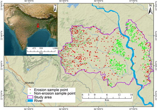
Nestled in the heart of eastern India, the Kangsabati River basin stands as a testament to the intricate interplay of geography and geology (Figure 1). This expansive tropical alluvial non-perennial river basin covers approximately 9658 km², stretching from latitude 21° 45′ N to 23° 30′ N and longitude 85° 45′ E to 88° 15′ E. Encompassing regions in West Bengal and southeastern Jharkhand, the basin’s drainage pattern is characterized by the convergence of various tributaries, including Kumari, Bhairabbanki, and Taraphini, forming a dendritic to sub-dendritic network. Geological complexities abound, with sixteen formations shaping their hydro-geological and lithological composition, resulting in diverse landscapes from ancient Achaeans to the vibrant Tertiary-Quaternary formations. The basin experiences the rhythm of tropical monsoons, with rainfall varying from 1077 to 1804 mm/year, predominantly during the monsoon season. The terrain unfolds in three distinct physiographic sites—plateau fringe, undulating topography, and low land surface—each contributing to varying erosion susceptibilities. The northern segment aligns with the Chota Nagpur Plateau, while the southern plains showcase alluvial deposits. The basin’s geological diversity is mirrored in its soil composition, boasting fine loamy ultipaleustalfs shaped by geological heritage and climatic influence. Amidst these intricacies, the Kangsabati basin offers a captivating narrative of India’s geographical diversity, where the symphony of geological formations, climatic nuances, and drainage patterns orchestrates the intricate dance of soil erosion dynamics.

Figure 1. Location of the study area.

2.2. Data source

In this study, data from the Shuttle Radar Topography Mission (SRTM) (https://www.usgs.gov) were used to develop critical terrain features such as a detailed elevation model, slope analysis, and additional topographic elements that were critical to analysing the geographic features of the study area. In addition, a Land Use and Land Cover (LULC) map derived from Sentinel-2 satellite imagery provided by ESRI (https://www.arcgis.com/home/index.html) in 2021 was used for the study. The soil taxonomy data used in our analysis was digitized from the West Bengal Soil Sheets No. 2, 3, and 4, originally compiled by the National Bureau of Soil Survey and Land Use Planning in collaboration with the Department of Agriculture, Government of West Bengal (http://www.nbsslup.in/). The K factors were then computed using a soil erodibility nomograph, as detailed in previous studies conducted within the same geographical region (Bhattacharya et al. 2021). In addition, an extensive dataset from the Indian Meteorological Department (IMD) covering a period of 40 years (1980-2020) was used to collect rainfall data for the study.

2.3. Method for estimating potential soil erosion

To estimate potential soil erosion, the Revised Universal Soil Loss Equation (RUSLE) is used in a Geographic Information System (GIS) environment, in particular ArcGIS. RUSLE is an empirical model that quantifies the average annual soil loss taking into account various environmental factors. The methodology comprises two main steps: the preparation of a gridded data set and the modelling of potential soil erosion.

2.3.1. Preparation of gridded dataset for potential soil erosion modeling

The preparation of a gridded dataset for modelling potential soil erosion in ArcGIS begins with the systematic collection of spatial data relevant to each factor of the Revised Universal Soil Loss Equation (RUSLE) (Phinzi et al. 2021). This involves a careful process of data collection and transformation to ensure accuracy in soil erosion susceptibility modelling. The rainfall erosivity factor (R-factor) is important to measure the kinetic energy of rain, a critical component in triggering soil detachment (Negese et al. 2021). It is quantified in units of MJ mm ha⁻¹ h⁻¹yr⁻¹ and derived from historical precipitation data (Negese et al. 2021). The spatial representation of the R-factor is based on the IDW (Inverse Distance Weighted) method, which ensures a continuous surface that accurately reflects the different erosion values influenced by precipitation intensity. The K-factor reflects the susceptibility of the soil to erosion and is assessed on the basis of soil type characteristics. It is measured in units of t ha h ha⁻¹MJ⁻¹mm⁻¹ (Mohammed et al. 2020a, 2020b). Soil maps are used to interpolate K-factor values and provide a standardised view of erosion potential under different soil conditions. The LS factor, which represents the topographical influence on erosion, is calculated from a digital elevation model (DEM) (Ahmed et al. 2024). This dimensionless factor takes into account the length and steepness of slopes, which are decisive for the aggravation of soil erosion risk in sloping terrain. The calculations are performed using the Flow Accumulation and Slope tools in ArcGIS, which translate topographic data into potential erosion patterns. The C-factor is derived from land use and vegetation data and illustrates the protective function of the vegetation cover against soil erosion (Ahmed et al. 2023). This dimensionless factor indicates the ratio of soil loss under certain cover conditions to the loss observed under bare fallow land. It is determined by classifying satellite imagery and analysing indices such as the Normalised Difference Vegetation Index (NDVI), then assigning C-values based on land cover types to indicate their erosion control effectiveness. The Supporting Practises Factor (P-factor) evaluates the effectiveness of erosion control measures, such as contouring or strip cropping (Ahmed et al. 2023a). The P-factor, which is also dimensionless, represents the ratio between the soil loss due to certain supporting practises and the loss due to conventional upward and downward cultivation of slopes. It is usually presented as a categorical data plane, which is later converted into a continuous, gridded format.

The aforementioned datasets are carefully processed and standardised into a raster format with a uniform cell size of 30 metres. This facilitates integrated analysis and ensures that the dataset is optimally configured for high-resolution modelling of soil erosion under different geographical and environmental conditions. Through this rigorous methodology, the study creates a robust framework for predicting areas prone to soil erosion, helping to strategically plan and implement effective soil protection measures.

2.3.2. Method for modeling gridded potential soil erosion using RUSLE

Once all factors are gridded and scaled accordingly, they are combined using the raster calculator to estimate the potential soil erosion for each grid cell (Ahmed et al. 2024). In the modelling phase, each factor is processed by spatial analysis tools in ArcGIS. The equation for estimating the average annual soil loss (A) is: (Equation-1) $$\mathrm{A}=\mathrm{R}\times \mathrm{K}\times \text{LS}\times \mathrm{C}\times \mathrm{P}$$(Equation-1)

Each rasterised layer is overlaid to perform a cell-by-cell multiplication using the ArcGIS raster calculation tool to produce a comprehensive map of soil erosion risk. The result is a predictive map that spatially represents the average annual rate of soil erosion in tonnes per hectare per year.

2.4. Verification of soil erosion model with ground truth and creation of soil erosion inventory

The verification of the soil erosion model by ground truthing is a crucial step to ensure its accuracy and reliability. In the method described, an inventory of potential soil erosion sites was created by visiting and digitising 80 sites as polygons suspected of significant erosion. These polygons were then converted into a raster format with a spatial resolution of 30 meters. This raster layer was then converted into a point file containing 3,680 discrete points. These points were overlaid with the raster layers of potential soil erosion derived from the RUSLE model. The comparison showed that 84% of the ground-truth sample points coincided with raster pixels indicating erosion rates of over 15 tonnes per hectare per year, confirming that the predictions of the RUSLE model were satisfactory and consistent with conditions on the ground. These points, representing areas where soil erosion is present, thus form a ‘presence’ dataset for soil erosion.

For robust binary classification in subsequent probability modelling, an equal number of ‘absence’ or negative samples are required where no soil erosion occurs. These were determined by analysing historical Google Earth imagery and validated by field visits to ensure a balanced representation of erosion and non-erosion sites. This comprehensive inventory, which includes data on both the presence and absence of soil erosion, is critical to the development of a classification-based model for predicting soil erosion probability. The binary nature of the target variables facilitates the application of different machine learning algorithms to classify areas into the categories ‘likely to erode’ or ‘unlikely to erode’, thus providing a valuable tool for planning soil protection and mitigation measures.

2.5. Preparation of gridded dataset for soil erosion probability modeling

Our methodology for preparing the raster dataset for soil erosion susceptibility modelling is carefully aligned with the RUSLE model to ensure the accuracy and relevance of our analysis (Figure 2). The RUSLE model, which is central to the assessment of erosion, requires accurate data on topography, soil properties, climate, vegetation and land management practises, which are included in the LS, K, R, C and P factors. Our selection and spatial representation of the 17 parameters, including elevation, soil type, precipitation, land use and slope, have been rigorously structured to reflect these factors. For example, elevation data from DEMs are included in the LS factor, while soil types and their erodibility index correspond to the K factor. Precipitation data interpolated to represent spatial variability defines the R-factor, and LULC data determines the C-factor. Reconciling our dataset preparation with the RUSLE parameters ensures that our model comprehensively captures the complex dynamics of soil erosion processes, improving the predictive accuracy and scientific validity of our vulnerability analysis. This alignment is crucial for the accurate quantification and spatial delineation of erosion risk, enabling targeted soil protection and management strategies.

Figure 2. Composite representation of environmental variables in a gridded dataset for soil erosion probability modeling, displaying topographic, climatic, and anthropogenic factors, such as a) elevation, b) K factor, c) LS factor, d) rainfall, e) LULC, f) slope, g) TWI, h) SPI, i) soil moisture, j) drainage. k) Profile curvature, l) plan curvature, m) aspect, n) NDVI, o) LST, p) NDWI and q) road density.

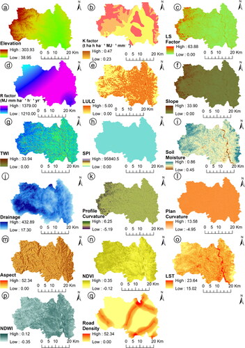
Elevation data, usually from a Digital Elevation Model (DEM), is used to derive various other topographic factors. In ArcGIS, elevation is represented as a continuous raster, with each cell having a value corresponding to the elevation above sea level. Elevation influences microclimate, vegetation patterns and water flow, all of which are factors in erosion. Soil type influences the ability of the soil to resist erosion (K-factor in RUSLE)). This raster is created by classifying areas based on soil types and their respective erodibility values. High values indicate erodible soils. The LS factor represents both the slope length and the steepness. In ArcGIS, the LS factor is calculated from the DEM using algorithms that simulate water flow and water accumulation. The precipitation data is crucial for the calculation of the R-factor in RUSLE These data are interpolated from point measurements to a continuous surface that represents the variation in precipitation erosivity. LULC data influence the C-factor in RUSLE. They are obtained from satellite images or aerial photographs and classified into different land cover types in ArcGIS. The slope is derived directly from the DEM in ArcGIS and affects the LS factor. Steeper slopes generally lead to higher erosion rates. TWI is a measure of the moisture potential of the soil and is calculated in ArcGIS using the DEM. It influences how much water accumulates in a given area and affects soil saturation and runoff potential. The SPI (Stream Power Index) indicates the erosive force of flowing water and is derived from the DEM in ArcGIS. Higher values correlate with a greater potential for erosion by watercourses. Soil moisture content can be estimated from satellite data or modelled in ArcGIS. It affects soil cohesion and susceptibility to erosion. Drainage patterns derived from hydrological analysis in ArcGIS affect how quickly water is drained from an area and thus influence erosion rates. Profile curvature influences the acceleration and deceleration of water flow on slopes. It is calculated from the DEM and influences the erosion risk by affecting the runoff velocity. Similar to profile curvature, plan curvature affects the flow path of water over a surface and is calculated from the DEM. Aspect determines the direction in which a slope faces and is derived from the DEM. It can influence microclimatic conditions and vegetation, which affects the risk of erosion. NDVI from remote sensing data indicates the condition and density of vegetation and affects the C-factor in erosion models. LST (Land Surface Temperature) can be an indicator of soil moisture and vegetation cover. It is derived from thermal satellite images. NDWI (Normalized Difference Water Index) is used to monitor moisture content in vegetation and soil. It is calculated from multispectral remote sensing data. Roads can contribute to soil compaction and alter drainage patterns, affecting erosion risk. Road density is quantified using spatial analysis tools in ArcGIS.

Each raster layer is processed to have the same cell size (30-metre spatial resolution), extent and coordinate system to ensure compatibility. The final gridded dataset serves as input for soil erosion probability modelling, where machine learning algorithms or statistical models can be applied to predict erosion risk based on the interactions between these variables.

2.6. Proposing Bayesian optimized hybrid deep learning models for soil erosion probability model

To harness the predictive power of machine learning for modelling soil erosion probability, a Bayesian-optimised hybrid deep learning model can be developed with different architectures, e.g. Deep Neural Networks (DNNs), Convolutional Neural Networks (CNNs), Fully Connected Neural Networks (FCNNs) and a hybrid of DCNN and CNN. These models are optimised using a Bayesian optimisation process to find the best hyperparameters that improve model performance.

2.6.1. Deep neural network

A DNN is a feedforward neural network with multiple hidden layers between the input and output layers (Talukdar et al. 2023). Each dense layer consists of numerous neurons, and the ReLU activation function introduces nonlinearity so that the model can learn complex patterns from the data (Ahmed et al. 2023a). The batch normalisation process normalises the input layer by adjusting and scaling the activations (Mallik et al. 2023). The dropout technique randomly drops units (along with their connections) from the neural network during training to prevent overfitting (Ahmed et al. 2023a). This structure allows the DNN to serve as a robust classifier for the probability of soil erosion by mapping the input features (e.g. slope, soil type, precipitation) to the output layer, that classifies the pixel as erosion-prone or not (Mallik et al. 2023). The sigmoid function in the output layer ensures that the final prediction is a probability between 0 and 1. The model is optimised using the Adam optimiser, a stochastic gradient descent method that adjusts the weights to minimise the binary cross-entropy loss, which gives the error in the predictions for a binary classification problem.

2.6.2. Convolutional neural network

The CNN works with gridded topological data, such as satellite images or spatial grids representing soil features (Talukdar et al. 2023). The convolutional layers apply a series of filters to the input data, which is then pooled (down-sampled) to reduce dimensionality and computational complexity. This process helps to detect local connections of features and patterns that are invariant to the location in the input space, which is essential for identifying areas at risk of erosion. The flattened output of the convolutional layers is then passed through dense layers, culminating in a sigmoid output layer for binary classification. This architecture is excellent for capturing spatial hierarchies and local features such as edges, textures, or specific patterns related to soil erosion, making it valuable for analysing spatial data.

2.6.3. Fully connected neural network

The FCNN is characterized by dense layers where each neuron is connected to every neuron in the preceding and subsequent layer, forming a fully connected network. The simplicity of the FCNN, with fewer layers and more neurons in each layer, can be quite effective for datasets where the input-output relationship is more direct and less complex. The model uses dropout after each layer to reduce overfitting, similar to the DNN. The FCNN is beneficial for soil erosion modeling when the input features have a clear and strong predictive relationship with soil erosion occurrence without the need for recognizing spatial or sequential patterns.

2.6.4. Proposed hybrid DNN-CNN model

The hybrid model combines the strengths of DNN and CNN architectures. It begins with a convolutional layer to process the input data, capturing any spatial relationships, followed by max pooling and flattening. Then, the model includes dense layers, like a traditional DNN, to learn the high-level features extracted by the convolutional layers. The hybrid DNN-CNN model utilises the capabilities of both architectures to effectively process spatial and non-spatial data. It starts with convolutional layers to process spatial data and identifies local features relevant to erosion risk. These features are then integrated and abstracted through the dense layers of the DNN. The hybrid model is particularly beneficial for modelling soil erosion as it can interpret complex patterns in both spatial data (such as the shape and texture of landscape features) and non-spatial data (such as soil chemistry or precipitation data). This dual approach allows the model to make more accurate and robust predictions about the likelihood of soil erosion because it can learn from the variety of features that contribute to erosion risk.

2.6.5. Bayesian optimization process

For each model, Bayesian optimization is used to find the optimal hyperparameters. This involves defining a search space for parameters such as the number of neurons in each layer, learning rate, dropout rate, number of filters, and kernel size. The optimization process uses the ‘hyperopt’ library with the Tree-structured Parzen Estimator (TPE) algorithm. A loss function, which typically is the negative accuracy or the binary cross-entropy loss on a validation set, is defined. The ‘fmin’ function from ‘hyperopt’ is then used to search through the hyperparameter space to find the set of parameters that minimizes the loss function. The optimization is done over a defined number of evaluations (‘max_evals’), and the best parameters are chosen based on the performance of the model during these trials. Each optimization process creates a ‘Trials’ object that records all the evaluation results, which can be analyzed to understand the hyperparameter efficiency and convergence of the optimization process. By using Bayesian optimization, the model is better suited to predict soil erosion probabilities with a higher level of accuracy and generalization capability.

2.7. Accuracy assessment of DL models

Accuracy assessment of deep learning models for soil erosion probability involves evaluating the performance of the classifier in distinguishing between eroded and non-eroded areas. The Receiver Operating Characteristic (ROC) curve and the Area Under the Curve (AUC) are pivotal for this evaluation (Jaydhar et al. 2022). The ROC curve is a graphical plot that illustrates the diagnostic ability of a binary classifier system as its discrimination threshold is varied (Pal et al. 2022). It plots the True Positive Rate (TPR, or recall) against the False Positive Rate (FPR) at various threshold settings (Ruidas et al. 2023). The AUC score provides a single measure of overall accuracy that is independent of a particular threshold; an AUC score of 1 represents a perfect model, while an AUC score of 0.5 indicates no discriminative power. Alongside ROC and AUC, a confusion matrix is another essential tool for accuracy assessment. It is a table used to describe the performance of a classification model on a set of test data for which the true values are known. It categorizes predictions into four types: true positives (TP), true negatives (TN), false positives (FP), and false negatives (FN). By setting a threshold (e.g. 0.5), continuous model predictions are converted into binary labels, which are then plotted in a confusion matrix. This matrix provides a detailed breakdown of the model’s performance, including errors.

Other crucial metrics derived from the confusion matrix include accuracy, precision, recall, and F1 score. Accuracy is the proportion of true results (both true positives and true negatives) among the total number of cases examined. Precision is the ratio of TP to all positive predictions (TP + FP) and measures the model’s exactness. Recall, also known as sensitivity or TPR, is the ratio of TP to all actual positives (TP + FN) and measures the model’s completeness. The F1 score is the harmonic mean of precision and recall and is a single metric that combines both aspects, providing a balance between precision and recall in the model’s evaluation. These metrics collectively provide a comprehensive picture of the model’s predictive performance and are critical for validating deep learning models applied to soil erosion probability modeling.

2.8. Method for SHAP for interpreting soil erosion probability models for better decision-making

SHAP (SHapley Additive exPlanations) is a game theory-based approach for interpreting predictive models, which assigns each feature an importance value for a particular prediction (Ahmed et al. 2024). In the context of soil erosion probability models, SHAP values provide insights into how each feature contributes to the model’s output, thereby demystifying complex model predictions (Ahmed et al. 2023a). It uses the classic Shapley values from cooperative game theory to fairly distribute the ‘payout’ (prediction) among the ‘players’ (features). Applying SHAP to soil erosion models involves computing the contribution of each input feature (like rainfall, slope, vegetation cover) to the probability of erosion. This is critical for decision-making as it helps in identifying the most influential factors contributing to erosion risk, allowing for targeted mitigation strategies. By interpreting the model with SHAP, stakeholders can understand the underlying factors that drive the model predictions, prioritize areas for soil conservation efforts, and make informed decisions to deploy resources effectively for erosion prevention. The transparency afforded by SHAP in interpreting complex deep learning models can lead to greater trust and adoption of these models in practical soil erosion management.

3. Results

3.1. Analysis of spatial gridded parameters of potential soil erosion

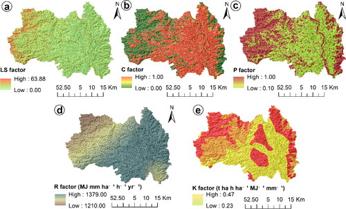
The parameters of the RUSLE model—LS, C, P, R and K—- are integrated to delineate soil erosion risks within a landscape (Figure 3). The LS factor, which indicates the potential for soil displacement due to slope length and steepness, shows pronounced variability throughout the study. The north-eastern section in particular has the highest LS values at 63.88, which indicates a significantly increased erosion potential on the steeper slopes. In contrast, the areas in the south and south-east have LS values approaching the lower end of the scale, indicating more moderate topographic slopes and potentially lower erosion processes. The protective role of vegetation cover against erosion is quantified by the C-factor, with dense vegetation in the southeast quadrant correlating with minimum values close to 0, indicating robust vegetation cover and an associated lower probability of erosion. Conversely, the northwestern regions are characterised by higher C-factor values approaching 1, indicating sparse vegetation and greater susceptibility to erosive forces. The P-factor, which indicates the effectiveness of soil protection measures, ranges between 0.1 and 1. Higher values, especially in the southwestern part of the area, indicate insufficient erosion control measures and point to regions where soil protection measures should be prioritised. The precipitation erosivity quantified by the R-factor varies between 1210 and 1379 MJ mm/ha/h/year, with the upper range of values occurring mainly in the north-western sector. This indicates an increased risk of erosion due to rainfall, which is confirmed by the observed erosion patterns and requires targeted measures. The erodibility of the soil, expressed by the K-factor, shows a range between 0.23 and 0.47 t ha/MJ/mm. The central areas show the lower K values, indicating more erosion-resistant soils, while the peripheral areas, especially in the north-east and south-west, show higher K values. These regions, characterised by more erosion-prone soils, are consistent with the observed higher erosion rates, suggesting that land use and soil management practises in these areas deserve immediate and special attention. The integration of these quantitative analyses shows that the overall erosion risk is significantly higher in the northwestern and northeastern parts of the study area, where the LS, R and K factors converge and imply an increased potential for soil loss.

Figure 3. Spatial distribution of RUSLE factors across the study area displaying (a) the LS factor, (b) C factor, (c) P factor, (d) R factor, and (e) K factor.

3.2. Estimation of potential soil erosion

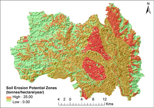
Potential soil erosion rates are expressed in tonnes per hectare per year, with a scale from 0 to 25. The colour-coded map indicates areas with different erosion risks: Regions with high erosion potential are shown in red, while regions with low erosion potential are green (Figure 4). Scientific quantification of the results shows that areas with prominent red shades, particularly in the north-east and north-west of the region, indicate high potential soil erosion rates approaching the upper limit of 25 tonnes per hectare per year. This correlates with high LS factors in these areas, indicating steep slopes where soil particles are more likely to be detached and transported by water. The red regions could also correspond to high C-factor values, which indicate minimal vegetation cover and thus a higher susceptibility to erosion. Conversely, areas with predominant shades of green, especially in the southern and south-eastern regions, are likely to have lower erosion rates, possibly close to the lower limit of the scale. These areas might benefit from dense vegetation (low C-factor) and are less affected by topographic steepness (low LS-factor), hence the lower erosion rates. The centre part of the map with a mixture of green and yellow indicates a moderate erosion risk, probably due to a combination of medium LS values and variable vegetation cover (C-factor). These areas may have lower K values, indicating soil types that are less susceptible to erosion, or effective cultivation practises (P-factor) that reduce the overall erosion potential.

Figure 4. Spatial estimation of potential soil erosion rates in the Kangsabati River basin using the RUSLE model, expressed in tonnes per hectare per year.

Development of spatial soil erosion probability model by integrating DL models and geospatial database

3.2.1. Assessment of geospatial database for soil erosion probability model

Soil erosion probability modelling integrates multiple parameters to assess and predict erosion risk in landscapes. Using 17 parameters, including topography, climate, land cover and anthropogenic factors, the model aims to identify areas prone to soil erosion and develop soil conservation strategies. The analysis of the parameters quantifies the erosion risk in the entire study area. Elevation indicates a higher risk in the northern elevations due to the increased runoff potential, with elevations ranging up to 303.93 meters. Soil erodibility ranges from 0.23 to 0.47, indicating that the western regions are more susceptible to erosion. Steep slopes with LS values of up to 63.88, especially in the north-east and south-west, increase the erosion potential. The precipitation erosivity between 1210.63 and 1379.93 indicates higher precipitation-induced erosion in the west. The land cover with a LULC index of up to 5 and sparse vegetation, especially in the south-east, increases the probability of erosion. Slope gradients and hydrological indices such as TWI and SPI indicate that central to northern valleys and watercourses are at risk. Soil moisture with values up to 0.86 indicates central regions at risk due to lower cohesion. Drainage, curvature metrics and aspect further delineate areas where water dynamics contribute to erosion risk, particularly in the north-west. Vegetation conditions and moisture indices highlight erosion risk at the eastern and western edges due to temperature and moisture fluctuations. The high road density indicates possible erosion near urban areas. Therefore, the northern and north-eastern highlands, steep slopes and western regions with intense rainfall are most vulnerable to erosion. In contrast, the southern and south-eastern areas with dense vegetation and well-drained soils are more resistant to erosion. The western and south-western areas, which are characterised by erodible soils and significant human disturbance, are also classified as vulnerable and require targeted erosion control measures.

3.2.2. Optimization of DL models for soil erosion probability modeling

Optimising DL models for modelling soil erosion probability is crucial for improving model performance and ensuring accurate predictions. Hyperparameter tuning is an essential part of this process, which involves selecting the best set of parameters to minimise the loss function. This process is facilitated by libraries such as skopt, which use Bayesian optimisation methods to efficiently navigate the hyperparameter space. The goal is to find a combination of parameters that yields the highest validation accuracy or the lowest validation loss, which indicates the model’s ability to generalise to unseen data.

For the DNN, the search space is defined as follows: the number of units in the first layer ‘n_units_1' ranges from 16 to 256, in the second layer ‘n_units_2' from 64 to 512 and in the third layer ‘n_units_3' from 16 to 256. The learning rate is searched on a logarithmic scale from 0 to 0.1, the dropout rate from 0.2 to 0.5, the number of layers from 2 to 5 and the batch size from [32, 64, 128, 256]. For the FCNN, the search space includes ‘n_units_dense_1' and ‘n_units_dense_2' each from 32 to 512, the learning rate on a logarithmic scale from 10^-9 to 10^-2, ‘dropout_rate_fcnn’ from 0.1 to 0.5 and ‘batch_size’ from 32 to 256. The hyperparameter search space of the CNN is defined with ‘n_filters_1' and ‘n_filters_2' from 16 to 128, ‘kernel_size_1' and ‘kernel_size_2' from 2 to 5, the learning rate on a logarithmic scale from 10^-9 to 10^-2, ‘dropout_rate’ from 0.1 to 0.5 and ‘batch_size’ from 32 to 256. The search space of the hybrid DNN-CNN model combines aspects of DNN and CNN, where ‘n_units_dense_1' and ‘n_units_dense_2' range from 32 to 512, ‘n_filters’ from 32 to 128, ‘filter_size’ from 3 to 10, the learning rate on a logarithmic scale from 10^-9 to 10^-2, ‘dropout_rate_dnn’ from 0.1 to 0.5 and ‘batch_size’ from 32 to 256.

The convergence diagrams illustrate (Figure 5) the optimisation process over 50 trials for each model. In these diagrams, the best target value (loss function) is plotted against the number of trials. In the beginning, the target value drops steeply as significant improvements in the hyperparameters are discovered. As the trials progress, the improvements become marginal and the graphs flatten out. This shows that the optimisation converges to a set of hyperparameters that offer the least loss. This shows that all models are well-tuned and tailored to the specifics of predicting soil erosion probability, which increases their usefulness in decision-making.The best hyperparameters resulting from the optimisation process for each model are as follows:

Figure 5. Convergence plots illustrating the optimization process over 50 trials for four distinct deep learning models employed in soil erosion probability modeling. Sub-figure (a) represents the optimization trajectory for the Deep Neural Network (DNN), sub-figure (b) for the Convolutional Neural Network (CNN), sub-figure (c) for the Fully Connected Neural Network (FCNN), and sub-figure (d) for the hybrid DNN-CNN model.

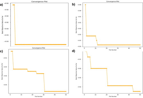
For the DNN, the best hyperparameters are a batch size of 32 (batch_size: 0), a dropout rate of approximately 0.316, a learning rate of approximately 0.023, 5 layers (n_layers: 5) with 252, 428 and 77 neurons in the first, second and additional layers, respectively. The optimal hyperparameters of the FCNN are a batch size of 97, a dropout rate of about 0.143, a learning rate of 0.0045 and 382 and 309 neurons in the dense layers. For the CNN, the model performs best with a batch size of 77, a dropout rate of about 0.496, kernel sizes of 3, a learning rate of 0.000465, and 34 and 56 philtres in the convolutional layers. The best hyperparameters of the hybrid DNN-CNN model are a batch size of 217, a dropout rate of 0.349, a filter size of 4, a learning rate of 0.0023, 96 filters, and 315 and 153 neurons in the dense layers. These hyperparameters are the result of a thorough and systematic search process aimed at maximising the predictive accuracy of the deep learning models for soil erosion probability.

3.2.3. Evaluation of fitness of trained optimized models

Evaluating the fitness of trained optimised models is a crucial step in machine learning to ensure that the models not only capture the underlying patterns in the training data but also generalise well to new, unseen data. This fitness study helps prevent overfitting (where the model learns noise and details that are irrelevant to the prediction task) and underfitting (where the model is too simple to capture the underlying structures). The learning curves of the optimized trained models for modeling soil erosion probability: (a) CNN, (b) DNN, (c) FCNN, and (d) DNN-CNN provide a visual representation of the learning process of the model over each epoch during training. Each model demonstrates effective learning and minimal overfitting, which indicates robust model training and reliable predictive performance (Figure 6). The validation loss reflects this decline, but remains consistently higher than the training loss, indicating a certain overfitting. Nevertheless, the plateau of both curves indicates a balance between learning and generalisation. The accuracy curves confirm a stable high accuracy of over 88% for training and validation, indicating a well-fitted model. The DNN model initially shows a rapid decrease in loss and then a steady convergence, with the validation loss very close to the training loss, indicating good generalisation. Accuracy levels off at 90% after an initial steep increase, indicating robust performance. For the FCNN, the model loss initially drops more steeply and the validation loss is subject to larger fluctuations, which could indicate a model that is sensitive to the training data and may require additional regularisation. Nevertheless, the accuracy curve shows an upward trend and reaches almost 90%, indicating that the model effectively captures the relevant patterns. The hybrid DNN-CNN model shows an initial decrease in losses, with training and validation losses converging at a low value, indicating a model that is well-tuned and generalises well to validation data. The accuracy in both training and validation increases sharply and then levels off, with the accuracy in training slightly higher than the accuracy in validation, indicating a slight overfitting but overall excellent fitness of the model.

Figure 6. Learning curves depicting the training and validation loss and accuracy for the optimized models used in soil erosion probability modeling: a) CNN, b) DNN, c) FCNN and d) DNN-CNN.

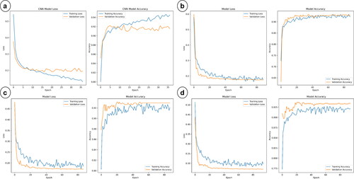
While all models exhibit favourable learning dynamics, the slight overfitting observed in the CNN model can be remedied through the introduction of regularization techniques such as dropout layers, augmentation of the training dataset to improve generalization, and the implementation of early stopping during training. These refinements will improve the robustness of the models for predicting soil erosion probability and ensure that they not only remain powerful but can also be reliably generalised to new data

3.2.4. Accuracy assessment of all DL models

The evaluation of the accuracy of DL models for modelling soil erosion probability can be comprehensively quantified using ROC curves, confusion matrices and performance metrics such as accuracy, precision, recall and F1-score. The ROC curves for the CNN, DNN, FCNN and DNN-CNN models (Figure 7) show excellent discriminatory power with AUC values of 0.98 for the CNN and DNN models and 0.97 for the FCNN and DNN-CNN models. These high AUC values indicate that all models have a high rate of true positives and a low rate of false positives at different threshold settings. The confusion matrices complement the ROC analysis by providing a detailed insight into the number of true positives and negatives as well as false positives and negatives (Figure 8). The matrices show that all models have a high number of true positives and true negatives, with relatively low false positives and false negatives, indicating consistently strong classification abilities.

Figure 7. ROC curves for deep learning models in soil erosion probability modeling, illustrating the trade-off between true positive rate and false positive rate: Sub-figures (a-d) display the ROC curves for the CNN, DNN, FCNN, and DNN-CNN models.

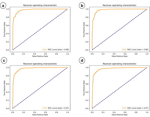
Figure 8. Confusion matrices for deep learning models in soil erosion probability modeling, showing the distribution of true positives, true negatives, false positives, and false negatives: Sub-figures (a-d) display the ROC curves for the CNN, DNN, FCNN, and DNN-CNN models.

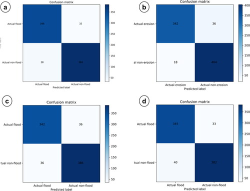
Quantitatively, the DNN model outperforms the others with an accuracy of 0.93, a precision of 0.92, a recall of 0.96 and an F1 score of 0.93 (Table 1). The high recall indicates that the DNN model is particularly good at recognising true erosion events, while the precision suggests that it produces fewer false positives. This is followed by the CNN model with a precision of 0.90, which lags behind the DNN model despite a high precision of 0.91 for recall and F1 score. The FCNN and DNN-CNN models show competitive results with an accuracy of 0.91 and 0.91 respectively, but do not achieve the high performance of the DNN model.

Table 1. Performance metrics for deep learning models in soil erosion probability prediction.

Model	Accuracy	Precision	Recall	F1-score
CNN	0.91	0.91	0.90	0.91
DNN	0.93	0.92	0.96	0.94
FCNN	0.91	0.93	0.90	0.91
DNN-CNN	0.91	0.91	0.93	0.92

Overall, although all models show high performance, the DNN model is quantitatively the best model for predicting soil erosion according to the specified metrics. Its balance of high precision and recall leads to the highest F1 score and makes it the most robust model among the models evaluated. The high accuracy of all models indicates a general ability to accurately predict soil erosion events, which is crucial for practical applications such as conservation planning and risk management.

3.3. Spatial soil erosion probability modeling

Spatial modelling of soil erosion probability using optimised DL models (Figure 9) illustrates the distribution of soil erosion risk across different zones. Analysing these models provides a quantitative assessment of areas with different erosion risks and allows us to identify specific directions where erosion probability is high. The CNN model predicts the largest area of very high erosion risk at 503.30 km², corresponding to 49.68% of the study area (Table 2). This significant coverage indicates extensive zones of potential land degradation, especially in the central and eastern regions where the red colour, indicating very high risk, is most pronounced. The DNN model provides a more diversified distribution with 225.81 km² (22.29%) categorised as very low risk, indicating a considerable area less prone to erosion, probably in the northern and western fringes. In addition, 222.73 km² (21.99%) are categorised as very high risk, indicating critical areas in the southern and south-eastern part of the study region. The FCNN model identifies 375.25 km² (37.04%) of the land as very low risk and 369.11 km² (36.43%) as very high risk, indicating two dominant zones with different erosion probabilities. The very high risk areas are clearly concentrated in the north-east and south-west, indicating regions where preventive measures should be prioritised. The DNN-CNN hybrid model shows a relatively more balanced distribution, with the highest proportion of the area falling under high risk (421.20 km², 41.58%). This model identifies critical zones mainly in the central to eastern sections of the map, where interventions to mitigate soil erosion may be most needed.

Figure 9. Spatial distribution of soil erosion susceptibility zones modeled by deep learning approaches: (a) CNN, (b) DNN, (c) FCNN, and (d) DNN-CNN.

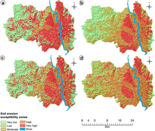
Table 2. Quantitative area coverage of soil erosion risk categories as predicted by different deep learning models.

Model		Area (in sq.km)	Area (%)
CNN	Very low	380.84	37.59
	Low	3.70	0.37
	Moderate	42.66	4.21
	High	82.61	8.16
	Very High	503.30	49.68
DNN	Very low	225.82	22.29
	Low	131.80	13.01
	Moderate	221.29	21.84
	High	211.48	20.87
	Very High	222.73	21.98
FCNN	Very low	375.25	37.04
	Low	30.24	2.99
	Moderate	71.89	7.096
	High	166.62	16.45
	Very High	369.11	36.43
DNN_CNN	Very low	12.42	1.23
	Low	312.71	30.87
	Moderate	54.56	5.39
	High	421.20	41.57
	Very High	212.24	20.95

Therefore, the DNN model tends to predict a more even distribution of soil erosion risk throughout the study area, while the CNN model identifies a larger part of the area as being at very high risk. The FCNN model makes a sharp distinction between very low and very high risk areas. The DNN-CNN hybrid model indicates a broad coverage with high erosion risk, especially in the eastern regions. The hybrid model appears to provide a nuanced view of erosion risk that may provide a more detailed guide to soil conservation measures. The models jointly emphasise the need for targeted erosion control strategies in the central to eastern regions, with potential high-risk areas also extending towards the south-east and north-east, consistent with the areas marked by red shades in the visual analysis.

3.4. Use of SHAP and variable importance for interpreting the optimized DL models for predicting soil erosion probability

The interpretation of deep learning models using SHAP values is important to understand the influence of different predictors on model results and to enable better decision-making by highlighting the most important factors for the probability of soil erosion. This interpretability bridges the gap between complex model predictions and actionable insights and facilitates targeted soil conservation strategies by highlighting the key drivers of erosion risk. The SHAP values provide information on the contribution of each feature to the prediction of the model. For all models (CNN, DNN, FCNN, DNN-CNN), the LULC and the soil erodibility factor (K-factor) consistently show a high influence on the model results, with the SHAP values indicating strong positive and negative effects on soil erosion predictions (Figure 10). This indicates that changes in land use and soil type significantly alter erosion risk, which is particularly important for managing these aspects to protect the soil. Quantitatively, the SHAP values span a range, with the CNN model showing SHAP values for LULC of up to about 0.15, indicating a strong effect of prediction. The DNN model also has SHAP values for LULC that reach almost 0.6, showing an even greater dependence on this feature. The FCNN and DNN-CNN models have SHAP values for LULC that are about 0.2 and 0.6, respectively.

Figure 10. SHAP value distributions for features across different deep learning models: (a) CNN, (b) DNN, (c) FCNN, and (d) DNN-CNN, depicting the impact of each predictor on the models’ output for soil erosion probability. Each dot represents the SHAP value for a feature for an individual prediction, with the color representing the feature value.

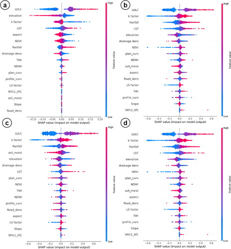
The mean absolute SHAP values illustrate the general importance of the features in the different models. For example, the most important features in the CNN model include LULC height and K-factor. The DNN model shows a similar pattern for LULC and K-factor, but places more emphasis on precipitation, indicating a model that heavily weights climatic influences on erosion. The FCNN model also prioritises LULC, K-factor and precipitation, indicating a balanced consideration of land management, soil properties and precipitation patterns. The DNN-CNN hybrid model emphasises the same key features, with LULC and the K-factor coming first, confirming the results of the individual CNN and DNN models.

Overall, the interpretation of these models via SHAP analysis shows that land management practices, soil characteristics and climatic conditions are key parameters influencing the probability of soil erosion. In particular, LULC and the K-factor emerge as dominant factors in all models, suggesting that they should be at the centre of soil erosion management and prevention strategies. The emphasis on these characteristics emphasises the need for targeted land use planning and soil conservation measures to reduce erosion risk. This analysis allows decision-makers to prioritise actions based on the features that most strongly influence soil erosion prediction.

4. Discussion

The current investigation of the use of Bayesian-optimised DL models to predict soil erosion probability represents a remarkable advance in the field of environmental science and land management. By carefully calibrating DL models such as DNN, CNN, FCNN and DNN-CNN using Bayesian optimisation and explaining model decisions with SHAP values, this research not only increases prediction accuracy, but also adds a level of interpretability to these models that is often lacking in complex environmental modelling. This integration of high computational power and transparency promotes enlightened, data-driven decision making in soil erosion control, fulfilling an important demand for sustainable land use practises. Our results highlight the effectiveness of DL models in spatial modelling of soil erosion, with the DNN model exhibiting significant predictive reliability as reflected in its accuracy and F1 score. A similarly high performance is seen for CNN and hybrid models, emphasising their utility for detailed spatial risk assessment.

The use of RUSLE estimates as the basis for soil erosion modelling in our study is consistent with traditional approaches such as those of Kebede et al. (2021) and Negese et al. (2021), who also used RUSLE in combination with GIS to estimate soil losses. Our analysis revealed significant erosion rates in the north-eastern and north-western regions, reaching up to 25 tonnes per hectare annually. This quantitative result is consistent with the region-specific analyses of Kebede et al. who highlighted the spatial variability of soil erosion risk in the Upper Beles watershed. Our research advances this approach by incorporating the RUSLE results into deep learning models to assess soil erosion probability, combining traditional erosion modelling with advanced computational techniques. This integration enables a more dynamic and nuanced analysis of erosion processes. It utilises RUSLE's strengths in providing baseline estimates of erosion and improves predictive capabilities through deep learning. Modelling susceptibility to soil erosion is central to identifying areas at risk and enabling targeted management strategies. Similar to Phinzi et al. (2021), who combined RUSLE with RF algorithms, our study used RUSLE output as a target variable for modelling soil erosion susceptibility. This integration bridges the traditional assessment of soil erosion with advanced computer modelling, providing a more sophisticated understanding of erosion risks.

The application of ML methods in soil erosion studies has gained momentum, with different researchers exploring different ML algorithms to predict erosion susceptibility. In our study, the use of deep learning models fine-tuned by Bayesian optimisation represents a significant development in soil erosion prediction methodology. For example, the DNN model demonstrated exceptional accuracy (0.93), precision (0.92) and F1 score (0.94), emphasising its robustness in identifying areas of high erosion risk. This model identified approximately 222.73 square kilometres as being at high risk of erosion, highlighting not only the precision of the model but also its spatial analysis capability. Such detailed and high-resolution insights into erosion susceptibility are a major advance over traditional methods, which often rely on broader, less specific data sets and analysis techniques. ML methods in soil erosion research have gradually evolved into more sophisticated and differentiated models. This transition is reflected in the work of Mosavi et al. (2020) and Bag et al. (2022), who used machine learning algorithms such as the Weighted Subspace Random Forest (WSRF) and RF, respectively, for soil erosion mapping. Ahmed et al. (2023) demonstrated a DNN model with an AUC of 0.98 and an F1 score of 0.97, indicating high predictive performance. Our study is in line with these results, showing a DNN model with an accuracy of 0.93 and an F1 score of 0.94, emphasising the robustness of DL in accurately predicting soil erosion. Furthermore, Saha et al. (2021) reported an AUC value of 0.93 for CNN models, confirming the potential of CNN in soil erosion studies. Models such as RNN, LSTM and GRU reported by Khosravi et al. (2023) and Gholami et al. (2023) also provide valuable insights, albeit with lower AUC values compared to DL models, indicating the superior performance of the latter in recognising complex spatial patterns related to soil erosion. Our research also followed this trend by implementing a range of deep learning architectures. Each model, from DNN to CNN and FCNN to hybrid DNN-CNN, was carefully optimised and evaluated to ensure high predictive performance and suitability for different aspects of erosion risk assessment. The CNN model, for example, was particularly adept at spatial analysis and identified 49.68% of the study area, or 503.30 square kilometres, as being at high risk of soil erosion. This ability to spatially delineate erosion-prone areas with high precision illustrates the strength of CNNs in capturing and interpreting complex spatial patterns in environmental data. Similarly, the FCNN model provided a balanced view of risk distribution across the study area by revealing both very low risk zones (37.04% or 375.25 km²) and very high risk zones (36.43% or 369.11 km²), providing a nuanced understanding of erosion susceptibility across different landscapes. The hybrid DNN-CNN model, which combines the strengths of DNN and CNN architectures, proved its effectiveness by identifying 41.58% of the area (421.20 km²) as high risk. This integration of different neural network architectures demonstrated the potential of hybrid models in capturing complicated spatial patterns and variability of soil erosion risk, providing a comprehensive and detailed overview of the erosion landscape. Overall, the use of advanced machine learning methods in our research represents a significant advance in the field of soil erosion prediction. By harnessing the computational power and analytical precision of deep learning, optimised by Bayesian methods, our study not only achieves high predictive accuracy, but also provides a deeper, more detailed spatial understanding of erosion risk. This approach is in line with the current trend in environmental modelling, which focuses on the use of sophisticated spatial models to achieve a more sophisticated and accurate prediction of environmental phenomena such as soil erosion.

The XAI and SHAP methods in our study significantly improve the scientific understanding and practical applicability of soil erosion prediction models. By integrating SHAP for model interpretation, similar to the strategies of Feng et al. (2021) and Zhou et al. (2022), our research goes beyond mere prediction of soil erosion and clarifies the underlying factors behind these predictions. This clarity is essential to turn the complicated modelling results into practical, actionable insights. Our SHAP value analysis has been instrumental in demystifying the influence of various predictors on the model results, thus promoting better decision making. For example, the analysis identified land use and soil type (LULC and K-factor) as key determinants of erosion predictions, which is consistent with empirical observations and theoretical expectations. The quantitative strength of SHAP values, which varies considerably from model to model, provides a nuanced view of how each factor contributes to erosion risk. In the CNN model, SHAP values for LULC showed a significant effect (up to about 0.15), while the DNN model showed an even stronger dependence on LULC, with SHAP values reaching almost 0.6. This variation in SHAP values between the different models (CNN, DNN, FCNN and DNN-CNN) not only highlights the different importance of features such as LULC and K-factor, but also emphasises the nuanced complexity within which these factors operate in the dynamics of soil erosion. The interpretability of the SHAP analysis bridges the gap between complex model predictions and actionable insights and facilitates targeted soil protection strategies by highlighting the main drivers of erosion risk. For example, the mean absolute SHAP values emphasised the overarching importance of features such as LULC, elevation and K-factor in all models, with some models additionally emphasising factors such as precipitation. This indicates a comprehensive consideration of land management practises, soil properties and climatic conditions in influencing soil erosion probability by the models. By highlighting the significant and varied influences of these factors, the SHAP analysis helps to prioritise soil conservation measures and land use planning strategies that are most likely to effectively mitigate soil erosion. The detailed insights from the SHAP values not only improve the interpretability of the models, but also enable decision-makers to focus on the most important factors and thus improve strategies to manage and prevent soil erosion. Therefore, the use of XAI and SHAP in our study underlines a methodological advance in soil erosion research that provides a rich, quantitatively orientated insight into the dynamics of soil erosion. This approach improves the decision-making process by providing precise, interpretable and actionable knowledge and thus represents an important contribution to environmental management and soil erosion prevention.

In order to effectively combat soil erosion in the study area, a detailed, site-specific strategy must be pursued. In the north-east, where erosion rates are approaching the upper limit, the strategy should include both biological and technical approaches. The biological component would include the strategic planting of native grasses and shrubs known for their soil-binding properties to strengthen the soil matrix and cover the soil. Agroforestry systems could be introduced, integrating tree species that improve soil structure and water retention. At the same time, technical measures such as gabion walls and terraces should be created to stabilise slopes and reduce the speed of surface runoff. In the north-west, similar biological measures could be complemented by the construction of retention dams in river channels to reduce flow energy and sediment transport. These structures can be designed to allow a controlled release of water and thus minimise the erosive force during runoff peaks. In the southern and south-eastern regions, where lower erosion rates are observed, the focus should be on maintaining and improving the existing vegetation cover. This can be achieved through controlled grazing and the promotion of sustainable agricultural practises, such as crop rotation and the use of organic farming methods that maintain soil health. In these areas, maintaining buffer strips of vegetation along watercourses can further prevent soil displacement. In the central region, where moderate erosion is observed, a mixture of these strategies should be applied. Conservation tillage can reduce soil disturbance and cover crops can be used in the off-season to protect the soil. The use of soil moisture conservation techniques, such as mulching and the use of water-retaining soil amendments, can increase the soil’s resistance to erosive forces. In all areas, it is important to integrate advanced soil monitoring systems that utilise the deep learning models developed in this study to continuously assess erosion risk. This data-driven approach can support the adaptive management of protection measures and ensure that they remain effective under changing environmental conditions. In addition, community involvement through soil conservation education programmes and the establishment of local conservation committees can promote a sense of responsibility and ensure the sustainability of erosion control strategies. By applying a comprehensive and science-based approach to soil erosion control, tailored to the specific needs of each area, the risk of soil degradation can be significantly reduced and the land preserved for future generations.

5. Conclusion

This research demonstrates a significant advancement in soil erosion prediction by integrating Bayes-optimised deep learning models with SHAP-based interpretability, improving both the accuracy and understandability of soil erosion probability predictions. Our careful analysis identified regions with a particularly high risk of erosion, with rates of almost 25 tonnes per hectare per year, especially in the north-eastern and north-western parts of the study area. The optimised DNN model exhibited exceptional performance metrics with an accuracy of 0.93 and an F1 score of 0.94, confirming its efficiency in identifying areas at risk of erosion. In addition, the CNN model identified almost half of the study area as being at high risk of erosion, indicating critical zones for intervention. The application of SHAP values to interpret these models showed that LULC and the K-factor have a decisive influence on soil erosion, with LULC contributing significantly to the predictive accuracy of the DNN model. These findings are of crucial importance for the development of targeted and effective soil protection strategies and thus for the promotion of sustainable land management practises worldwide.

The implications of this study go beyond the local or regional context and contribute to global efforts to combat soil degradation. By providing a methodological approach that can be adapted to different geographical settings, this study improves the global toolbox for environmental scientists and land managers. It supports the development of policies and conservation strategies aimed at maintaining soil health and preventing land degradation on a global scale. Although the limitations of predictive modelling, such as potential overfitting and dependence on data quality, are well known, this research paves the way for future studies that incorporate broader data sets, such as climate change projections. Furthermore, exploring the integration of real-time monitoring systems with predictive modelling could provide a more dynamic approach to managing and mitigating soil erosion risks globally. This comprehensive framework not only promotes scientific understanding, but also serves as a cornerstone for policy decisions and practical applications in soil conservation worldwide.

Author contributions

“All authors contributed to the study conception and design. Material preparation, data collection and analysis were performed by Meshel Alkahtani, Javed Mallick, Saeed Alqadhi, Md Nawaj Sarif, Mohamed Fatahalla Mohamed Ahmed, Hazem Ghassan Abdo. The first draft of the manuscript was written by Meshel Alkahtani, Javed Mallick, Saeed Alqadhi, Md Nawaj Sarif and all authors commented on previous versions of the manuscript. All authors read and approved the final manuscript.”

Availability data and materials

The data that support the findings of this study are available from the corresponding author upon reasonable request.

Acknowledgments

“The authors extend their appreciation to the Deanship of Scientific Research at King Khalid University for funding this work through Research Group under grant number RGP 2/442/44. The authors are also thankful to the USGS Earth Explorer for making the Landsat data freely available”.

Disclosure statement

No potential conflict of interest was reported by the author(s).

References

- Abdo HG. 2021. Estimating water erosion using RUSLE, GIS and remote sensing in Wadi-Qandeel river basin, Lattakia, Syria. ProcIndian Natl Sci Acad. 87(3):514–523. doi: 10.1007/s43538-021-00047-0.
- Abdo H, Salloum J. 2017. Mapping the soil loss in Marqya basin: Syria using RUSLE model in GIS and RS techniques. Environ Earth Sci. 76(3):114. doi: 10.1007/s12665-017-6424-0.
- Ahmed IA, Talukdar S, Baig MRI, Ramana GV, Rahman A, Shahfahad. 2024. Quantifying soil erosion and influential factors in Guwahati’s urban watershed using statistical analysis, machine and deep learning. Remote Sens Appl: Soc Environ. 33:101088. doi: 10.1016/j.rsase.2023.101088.
- Ahmed IA, Talukdar S, Islam ARMT, Rihan M, Malafaia G, Bera S, Ramana GV, Rahman A. 2023a. Contribution and behavioral assessment of physical and anthropogenic factors for soil erosion using integrated deep learning and game theory. J Clean Prod. 416:137689. doi: 10.1016/j.jclepro.2023.137689.
- Ahmed IA, Talukdar S, Naikoo MW, Parvez A, Pal S, Ahmed S, Rahman A, Islam ARMdT, Mosavi AH, Shahfahad, et al. 2023b. A new framework to identify most suitable priority areas for soil-water conservation using coupling mechanism in Guwahati urban watershed, India, with future insight. J Clean Prod 382:135363. doi: 10.1016/j.jclepro.2022.135363.
- Al-Najjar D, Al-Najjar H, Al-Rousan N, Assous HF. 2022. Developing machine learning techniques to investigate the impact of air quality indices on tadawul exchange index. Complexity. 2022(1):1–12. doi: 10.1155/2022/4079524.
- Arabameri A, Tiefenbacher JP, Blaschke T, Pradhan B, Tien Bui D. 2020. Morphometric analysis for soil erosion susceptibility mapping using novel gis-based ensemble model. Remote Sens. 12(5):874. doi: 10.3390/rs12050874.
- Aslam B, Maqsoom A, Alaloul WS, Musarat MA, Jabbar T, Zafar A. 2021. Soil erosion susceptibility mapping using a GIS-based multi-criteria decision approach: case of district Chitral, Pakistan. Ain Shams Eng J. 12(2):1637–1649. doi: 10.1016/j.asej.2020.09.015.
- Bag R, Mondal I, Dehbozorgi M, et al. 2022. Modelling and mapping of soil erosion susceptibility using machine learning in a tropical hot sub-humid environment. J Clean Prod. 364:132428.
- Bag R, Mondal I, Dehbozorgi M, Bank SP, Das DN, Bandyopadhyay J, Pham QB, Fadhil Al-Quraishi AM, Nguyen XC. 2022. Modelling and mapping of soil erosion susceptibility using machine learning in a tropical hot sub-humid environment. J Cleaner Prod. 364:132428. doi: 10.1016/j.jclepro.2022.132428.
- Barakat A, Rafai M, Mosaid H, Islam MS, Saeed S. 2023. Mapping of water-induced soil erosion using machine learning models: a case study of Oum Er Rbia Basin (Morocco). Earth Syst Environ. 7(1):151–170., doi: 10.1007/s41748-022-00317-x.
- Bhattacharya RK, Das Chatterjee N, Das K. 2021. Land use and land cover change and its resultant erosion susceptible level: an appraisal using RUSLE and logistic regression in a tropical plateau basin of West Bengal, India. Environ Dev Sustain. 23(2):1411–1446. doi: 10.1007/s10668-020-00628-x.
- Biswas T, Pal SC, Saha A, Ruidas D, Islam ARMT, Shit M. 2023. Hydro-chemical assessment of groundwater pollutant and corresponding health risk in the Ganges delta, Indo-Bangladesh region. J Cleaner Prod. 382:135229. doi: 10.1016/j.jclepro.2022.135229.
- Blake WH, Rabinovich A, Wynants M, Kelly C, Nasseri M, Ngondya I, Patrick A, Mtei K, Munishi L, Boeckx P, et al. 2018. Soil erosion in East Africa: an interdisciplinary approach to realising pastoral land management change. Environ Res Lett. 13(12):124014. doi: 10.1088/1748-9326/aaea8b.
- Chakrabortty R, Pal SC. 2023. Modeling soil erosion susceptibility using GIS-based different machine learning algorithms in monsoon dominated diversified landscape in India. Model Earth Syst Environ. 9(2):2927–2942. doi: 10.1007/s40808-022-01681-3.
- Chakrabortty R, Pal SC, Arabameri A, Ngo PTT, Chowdhuri I, Roy P, Malik S, Das B. 2022. Water-induced erosion potentiality and vulnerability assessment in Kangsabati river basin, eastern India. Environ Dev Sustain. 24(3):3518–3557. doi: 10.1007/s10668-021-01576-w.
- Chakrabortty R, Pal SC, Sahana M, et al. 2020. Soil erosion potential hotspot zone identification using machine learning and statistical approaches in eastern India. Netherlands: Springer.
- Chakrabortty R, Pradhan B, Mondal P, Pal SC. 2020. The use of RUSLE and GCMs to predict potential soil erosion associated with climate change in a monsoon-dominated region of eastern India. Arab J Geosci. 13(20):1073. doi: 10.1007/s12517-020-06033-y.
- Cheng Z, Lu D, Li G, et al. 2018. A random forest-based approach to map soil erosion risk distribution in Hickory Plantations in western Zhejiang Province, China. Remote Sens. 10:1899.
- Esmali Ouri A, Golshan M, Janizadeh S, Cerdà A, Melesse AM. 2020. Soil erosion susceptibility mapping in Kozetopraghi catchment, Iran: a mixed approach using rainfall simulator and data mining techniques. Land. 9(10):368. doi: 10.3390/land9100368.
- FAO. 2019. Soil erosion–the greatest challenge for sustainable soil management. Rome: FAO. 100 pp.
- Feng DC, Wang WJ, Mangalathu S, Taciroglu E. 2021. Interpretable XGBoost-SHAP machine-learning model for shear strength prediction of squat RC walls. J Struct Eng. 147(11):04021173. doi: 10.1061/(ASCE)ST.1943-541X.0003115.
- Flanagan DC, Ascough JC, Nearing MA, Laflen JM. 2001. The water erosion prediction project (WEPP) model. In: Harmon RS, Doe WW, editors. Landscape erosion and evolution modeling. Boston, MA: Springer. doi: 10.1007/978-1-4615-0575-4_7.
- Gayen A, Haque SM, Saha S. 2020. Modeling of gully erosion based on random forest using GIS and R. In: Shit P, Pourghasemi H, Bhunia G, editors. Gully erosion studies from India and surrounding regions. Advances in science, technology & innovation. Cham: Springer. doi: 10.1007/978-3-030-23243-6_3.
- Gholami H, Mohammadifar A, Golzari S, Song Y, Pradhan B., 2023. Interpretability of simple RNN and GRU deep learning models used to map land susceptibility to gully erosion. Sci Total Environ. 904:166960. doi: 10.1016/j.scitotenv.2023.166960.
- Ghosal K, Das Bhattacharya S. 2020. A review of RUSLE model. J Indian Soc Remote Sens. 48(4):689–707. doi: 10.1007/s12524-019-01097-0.
- Ghosh A, Maiti R. 2021. Soil erosion susceptibility assessment using logistic regression, decision tree and random forest: study on the Mayurakshi river basin of Eastern India. Environ Earth Sci. 80(8):1–16. doi: 10.1007/s12665-021-09631-5.
- Iban MC, Bilgilioglu SS. 2023. Snow avalanche susceptibility mapping using novel tree-based machine learning algorithms (XGBoost, NGBoost, and LightGBM) with eXplainable Artificial Intelligence (XAI) approach. Stoch Environ Res Risk Assess. 37(6):2243–2270. doi: 10.1007/s00477-023-02392-6.
- Igwe CA, Mbagwu JSC. 1999. Application of SLEMSA and USLE erosion models for potential erosion hazard mapping in South-Eastern Nigeria. Int Agrophysics. 13:41–48.
- Jaydhar AK, Pal SC, Saha A, Islam ARMT, Ruidas D. 2022. Hydrogeochemical evaluation and corresponding health risk from elevated arsenic and fluoride contamination in recurrent coastal multi-aquifers of eastern India. J Cleaner Prod. 369:133150. doi: 10.1016/j.jclepro.2022.133150.
- Kebede YS, Endalamaw NT, Sinshaw BG, Atinkut HB. 2021. Modeling soil erosion using RUSLE and GIS at watershed level in the upper beles, Ethiopia. Environ Challenges. 2:100009. doi: 10.1016/j.envc.2020.100009.
- Khosravi K, Rezaie F, Cooper JR, Kalantari Z, Abolfathi S, Hatamiafkoueieh J., 2023. Soil water erosion susceptibility assessment using deep learning algorithms. J Hydrol. 618:129229. doi: 10.1016/j.jhydrol.2023.129229.
- Kulimushi LC, Bigabwa Bashagaluke J, Prasad P, Heri-Kazi AB, Lal Kushwaha N, Masroor M, Choudhari P, Elbeltagi A, Sajjad H, Mohammed S, et al. 2023. Soil erosion susceptibility mapping using ensemble machine learning models: a case study of upper Congo river sub-basin. Catena. 222:106858. doi: 10.1016/j.catena.2022.106858.
- Li L, Wang Y, Liu C. 2014. Effects of land use changes on soil erosion in a fast developing area. Int J Environ Sci Technol. 11:1549–1562.
- Mallik S, Das S, Chakraborty A, Mishra U, Talukdar S, Bera S, Ramana GV. 2023. Prediction of non-carcinogenic health risk using Hybrid Monte Carlo-machine learning approach. Human and Ecol Risk Assess: An Int J. 29(3–4):777–800. doi: 10.1080/10807039.2023.2188417.
- Mohammed S, Abdo HG, Szabo S, Pham QB, Holb IJ, Linh NTT, Anh DT, Alsafadi K, Mokhtar A, Kbibo I, et al. 2020a. Estimating human impacts on soil erosion considering different hillslope inclinations and land uses in the coastal region of Syria. Water. 12(10):2786. doi: 10.3390/w12102786.
- Mohammed S, Alsafadi K, Talukdar S, Kiwan S, Hennawi S, Alshihabi O, Sharaf M, Harsanyie E. 2020b. Estimation of soil erosion risk in southern part of Syria by using RUSLE integrating geo informatics approach. Remote Sens Appl: Soc Environ. 20:100375. doi: 10.1016/j.rsase.2020.100375.
- Morgan P. 1984. The thermal structure and thermal evolution of the continental lithosphere. Phys Chem Earth. 15:107–193. doi: 10.1016/0079-1946(84)90006-5.
- Morgan RPC. 2001. A simple approach to soil loss prediction: a revised Morgan–Morgan–Finney model. Catena. 44(4):305–322. doi: 10.1016/S0341-8162(00)00171-5.
- Morgan RPC, Duzant JH. 2008. Modified MMF (Morgan–Morgan–Finney) model for evaluating effects of crops and vegetation cover on soil erosion. Earth Surf Process Landforms J Br Geomorphol Res Gr. 33:90–106.
- Morgan RPC, Quinton JN, Smith RE, et al. 1998. The European Soil Erosion Model (EUROSEM): a dynamic approach for predicting sediment transport from fields and small catchments. Earth Surf Process Landforms J Br Geomorphol Gr. 23:527–544.
- Mosavi A, Golshan M, Janizadeh S, et al. 2022. Ensemble models of GLM, FDA, MARS, and RF for flood and erosion susceptibility mapping: a priority assessment of sub-basins. Geocarto Int. 37:2541–2560.
- Mosavi A, Sajedi-Hosseini F, Choubin B, Taromideh F, Rahi G, Dineva AA. 2020. Susceptibility mapping of soil water erosion using machine learning models. Water. 12(7):1995. doi: 10.3390/w12071995.
- Mustafa MRU, Sholagberu AT, Yusof KW, Hashim AM, Khan MWA, Shahbaz M., 2018. SVM-based geospatial prediction of soil erosion under static and dynamic conditioning factors. MATEC Web Conf. 203:04004. doi: 10.1051/matecconf/201820304004.
- Nasidi NM, Wayayok A, Abdullah AF, Kassim MSM. 2020. Vulnerability of potential soil erosion and risk assessment at hilly farms using InSAR technology. Alger J Eng Technol. 3:1–8.
- Negese A, Fekadu E, Getnet H. 2021. Potential soil loss estimation and erosion-prone area prioritization using RUSLE, GIS, and remote sensing in Chereti Watershed, Northeastern Ethiopia. Air Soil Water Res. 14:117862212098581. doi: 10.1177/1178622120985814.
- Pal S. 2015. Identification of soil erosion vulnerable areas in Chandrabhaga river basin: a multi-criteria decision approach. Model Earth Syst Environ. 2(1):1–11. doi: 10.1007/s40808-015-0052-z.
- Pal SC, Ruidas D, Saha A, Islam ARMT, Chowdhuri I. 2022. Application of novel data-mining technique based nitrate concentration susceptibility prediction approach for coastal aquifers in India. J Cleaner Prod. 346:131205. doi: 10.1016/j.jclepro.2022.131205.
- Phinzi K, Ngetar NS, Ebhuoma O. 2021. Soil erosion risk assessment in the Umzintlava catchment (T32E), Eastern Cape, South Africa, using RUSLE and random forest algorithm. South African Geographical Journal. 103(2):139–162. doi: 10.1080/03736245.2020.1716838.
- Prasanth Kadiyala S, Woo WL. 2021. Flood prediction and analysis on the relevance of features using explainable artificial intelligence. In 2021 2nd Artificial Intelligence and Complex Systems Conference. p. 1–6. doi: 10.1145/3516529.3516530.
- Renard KG, Foster GR, Weesies GA, Porter JP. 1991. RUSLE, revised universal soil loss equation. J Soil Water Conserv. 46(1):30–33.
- Rose CW, Coughlan KJ, Fentie B. 1998. Griffith University Erosion System Template (GUEST). In Modelling soil erosion by water. p. 399–412, Springer Berlin Heidelberg.
- Ruidas D, Pal SC, Saha A, Chowdhuri I, Shit M. 2022. Hydrogeochemical characterization based water resources vulnerability assessment in India’s first Ramsar site of Chilka lake. Mar Pollut Bull. 184:114107. doi: 10.1016/j.marpolbul.2022.114107.
- Ruidas D, Pal SC, Towfiqul Islam ARM, Saha A. 2023. Hydrogeochemical evaluation of groundwater aquifers and associated health hazard risk mapping using ensemble data driven model in a water scares plateau region of eastern India. Expo Health. 15(1):113–131. doi: 10.1007/s12403-022-00480-6.
- Sadhasivam N, Bhardwaj A, Pourghasemi HR, Kamaraj NP. 2020. Morphometric attributes-based soil erosion susceptibility mapping in Dnyanganga watershed of India using individual and ensemble models. Environ Earth Sci. 79(14):1–28. doi: 10.1007/s12665-020-09102-3.
- Saha S, Gayen A, Pourghasemi H, Tiefenbacher J. 2019. Identification of soil erosion-susceptible areas using fuzzy logic and analytical hierarchy process modeling in an agricultural watershed of Burdwan district, India. Environ Earth Sci. 78(23):649. doi: 10.1007/s12665-019-8658-5.
- Saha S, Sarkar R, Thapa G, Roy J. 2021. Modeling gully erosion susceptibility in Phuentsholing, Bhutan using deep learning and basic machine learning algorithms. Environ Earth Sci. 80(8):1–21. doi: 10.1007/s12665-021-09599-2.
- Sarkar T, Mishra M. 2018. Soil erosion susceptibility mapping with the application of logistic regression and artificial neural network. J Geovisualization Spat Anal. 2(1):8. doi: 10.1007/s41651-018-0015-9.
- Shao K, Youssef K, Moon S, Bouchard L. 2019. Explainable AI landslide susceptibility modeling by superposable neural networks. In: AGU Fall Meeting Abstracts; p. EP43D–E2390.
- Silburn DM, Loch RJ. 1989. Evaluation of the CREAMS model. I. Sensitivity analysis of the soil erosion sedimentation component for aggregated clay soils. Soil Res. 27:545–561.
- Sinshaw BG, Belete AM, Tefera AK, Dessie AB, Bizuneh BB, Alem HT, Atanaw SB, Eshete DG, Wubetu TG, Atinkut HB, et al. 2021. Prioritization of potential soil erosion susceptibility region using fuzzy logic and analytical hierarchy process, upper Blue Nile Basin, Ethiopia. Water-Energy Nexus. 4:10–24. doi: 10.1016/j.wen.2021.01.001.
- Talukdar S, Ahmed S, Naikoo MW, Rahman A, Mallik S, Ningthoujam S, Bera S, Ramana GV, Shahfahad. 2023. Predicting lake water quality index with sensitivity-uncertainty analysis using deep learning algorithms. J Cleaner Production. 406:136885. doi: 10.1016/j.jclepro.2023.136885.
- Vogel H-J, Bartke S, Daedlow K, Helming K, Kögel-Knabner I, Lang B, Rabot E, Russell D, Stößel B, Weller U, et al. 2018. A systemic approach for modeling soil functions. SOIL. 4(1):83–92. doi: 10.5194/soil-4-83-2018.
- Wan A, Dunlap L, Ho D, et al. 2020. NBDT: neural-backed decision trees. arXiv Prepr arXiv200400221.
- Youssef K, Shao K, Moon S, Bouchard L-S. 2022. XAI model for accurate and interpretable landslide susceptibility. arXiv Prepr arXiv220106837.
- Yunkai L, Yingjie T, Zhiyun O, Lingyan W, Tingwu X, Peiling Y, Huanxun Z. 2010. Analysis of soil erosion characteristics in small watersheds with particle swarm optimization, support vector machine, and artificial neuronal networks. Environ Earth Sci. 60(7):1559–1568. doi: 10.1007/s12665-009-0292-1.
- Zhao Y, Gao G, Ding G, Wang L, Chen Y, Zhao Y, Yu M, Zhang Y., 2022. Assessing the influencing factors of soil susceptibility to wind erosion: A wind tunnel experiment with a machine learning and model-agnostic interpretation approach. Catena. 215:106324. doi: 10.1016/j.catena.2022.106324.
- Zhou X, Wen H, Li Z, Zhang H, Zhang W. 2022. An interpretable model for the susceptibility of rainfall-induced shallow landslides based on SHAP and XGBoost. Geocarto Int. 37(26):13419–13450. doi: 10.1080/10106049.2022.2076928.
- Ziadat FM, Zdruli P, Christiansen S, et al. 2022. An overview of land degradation and sustainable land management in the near East and North Africa. Sustain Agric Res. 11:11–24.