Identification of cropland in Tibetan Plateau based on time series remote sensing features

Abstract

Cropland is crucial for regional food security, especially in vulnerable areas like the Tibetan Plateau. Accurate monitoring was hindered of cropland distribution due to complex topography and diverse crop phenology, making it challenging to assess its agricultural sustainability. To address this, this study aimed to develop a cropland identification approach based on an optimal identification feature knowledge graph (OIFKG) derived from time series remote sensing data. Cropland OIFKG (C_OIFKG) enhanced cropland identification accuracy by 96.6%, with producer’s accuracy and user’s accuracy of 98.1% and 89.9% respectively for cropland. The total cropland area in the Tibetan Plateau for 2022 was estimated at 1,800,160 hectares, representing about 1% of the total land area, with a significant concentration in the northeastern Qinghai province and the Yarlung Zangbo River Valley of Tibet Autonomous Region. The total cropland area estimated in this study for the Tibetan Plateau lied within the range provided by two published land cover datasets, being 3.56% lower than one dataset and 16.4% higher than the other. The cropland identification approach proposed by this study reduced reliance on known samples, improving spatiotemporal generalization capability. In the Tibetan Plateau, where cropland distribution was exceedingly rare, the method still achieved promising performance in cropland identification, demonstrating its effectiveness on the assessment of agriculture sustainability in high-altitude regions with intricate landscapes. Moreover, further assessment of C_OIFKG's applicability in different regions and compatibility with multi-source remote sensing data is needed.

Keywords:

• Automated cropland mapping
• optimal identification feature
• knowledge graph
• remote sensing
• Tibetan Plateau

1. Introduction

Cropland has been an indispensable factor for the survival of human beings, and it provides critical significance for the sustainable development of regional agriculture, thereby ensuring the long-term stability and prosperity of the region. Given the rise in population and accelerated urbanization, it has become a crucial national strategy for the preservation and management of cropland. Consequently, the identification of cropland has emerged as an indispensable and practical issue. This particularly important in food-insecure regions like mountainous and hilly area, where characterizing agricultural production remains a major challenge. In Tibetan Plateau (TP), with the situation of global warming, the agricultural producing area has expanded significantly over the past few decades, which might induce desertification, degradation, and water supply loss (Zhang et al. 2013; Wang et al. 2019; Di et al. 2021). Thus, it is crucial to identify cropland accurately for monitoring of cropping intensities, crop types, crop health, and crop productivity, which is the basis of food security evaluation. However, the absence of cropland product in TP at high resolution and accuracy leads to great uncertainties and poor assessment of local sustainable development of agriculture (Xiong et al. 2017a, 2017b).

Due to the advantages of wide coverage, high efficiency, and low cost, remote sensing has emerged as a primary means for identifying cropland, thereby monitoring the distribution, extent, quality, and utilization of cropland, which can provide robust data support for agricultural practice and cropland management (Gallego et al. 2014; Hegazy and Kaloop 2015). A number of cropland products or land cover products (mapped cropland as one class) at global/national scale have been developed, mostly at a resolution between 1 km and 30 m (Friedl et al. 2010; Alcantara et al. 2012; Thenkabail and Wu 2012; Chen et al. 2015; Estel et al. 2015; Teluguntla et al. 2017; Zhang et al. 2020). However, it is questionable to use these products for practical purpose in specific region, cause estimates and spatial location of cropland based on different products are inconsistent (Fritz et al. 2011; Xiong et al. 2017b), especially in regions with complex topography and fragmented landscape like TP. Different definitions, resolutions of input data, and classification methods can all contribute to the aforementioned differences. Therefore, the uncertainties associated with cropland identification derived from these factors have a substantial impact on the accuracy of food security and sustainable development of agriculture assessment.

Traditional cropland identification has typically relied on manual visual interpretation, which can achieve high accuracy but time-consuming and labor-intensive, and making it impractical for broad-scale and high-efficiency applications (Buttner 2014; Xiong et al. 2017a). For automated cropland mapping, there are a number of approaches adopted, such as phenology based algorithms (Jeganathan et al. 2014; Dong et al. 2015; Di et al. 2021), classification regression trees (Egorov et al. 2015), support vector machines (Mountrakis et al. 2011; Yang et al. 2011), random forest (Teluguntla et al. 2018), and many other machine learning algorithms (including deep learning) (Tseng et al. 2008; Lary et al. 2016; Xu et al. 2020; Khan et al. 2021; Xie et al. 2023), each of which may have varying degrees of effectiveness depending on the specific scenarios and data available. Phenology based algorithms rely heavily on high-quality, continuous time series data which may be limited in mountainous regions prone to cloud cover. Machine learning techniques, while powerful, are often constrained by the scarcity of precise ground truth data for model training, particularly in remote and rugged terrains. In summary, in current cropland identification, especially in TP, there are many challenges, such as variable crop calendars, fragmented agricultural landscape, and spectral similarity with grassland, in addition, two practical challenges of data acquisition are inevitable. Firstly, the spatiotemporal heterogeneity of original effective satellite data (without cloud, fog, and shadow interference), meaning sufficient high-quality remote sensing data is limited by local climate conditions. Secondly, the lack of ground sample data, meaning the complex topography makes it difficult to conduct intensive ground surveys. These all may induce the aforementioned methods to identify cropland ineffective.

Given the above discussions, there is a clear gap in the development of a reliable cropland identification approach specifically tailored for mountainous and hilly area, such as TP. (1) current methods and products are not sufficiently precise for regions like TP, which have complex terrains and fragmented landscapes; (2) traditional methods are difficult to adapt to the spatiotemporal heterogeneity of original effective satellite data; (3) the identification process need to be free from the dependence on seasonal samples; (4) a specialized approach can better lead to more accurate large-scale cropland mapping. In conclusion, there is a pressing need for a cropland identification method that is specifically designed for challenging environments like TP. Such a method would greatly enhance the accuracy and timeliness of cropland monitoring, thereby supporting more effective agricultural management and contributing to the region’s food security and agricultural sustainability.

Thus, the overarching goal of this study is to develop and test cropland (land that are currently being cultivated with crops) identification with time series remote sensing features in TP. TP is chosen given its critical role in regional food security, where relatively fragile environmental conditions often have a severe impact on local agricultural activities. First, to capture the optimal identification features for cropland based on time series remote sensing images; Second, to clarify the temporal trend of the optimal identification features and construct a knowledge graph; Third, to identify cropland in TP based on the knowledge graph of optimal identification features.

2. Study area and data

2.1. Study area

The TP spans from approximately 25°59′37″–39°49′33″N and 73°29′56″–104°40′20E, and the Tibet Autonomous Region and Qinghai Province (T&Q) are regarded as the two most significant regions, which collectively encompass over 60% of the entire TP. As such, these regions were chosen as the primary focus of this study (Figure 1). The study area is characterized by significant changes in terrain, with average elevations ranging from 3000 to 5000 m (Yao et al. 2012). The climate varies widely across the study area due to its high altitude and complex topography. The annual average temperature of most of the region is lower than 0 °C, the annual average precipitation ranges from 100 mm to over 1000 mm, and given high altitude and clear skies, the annual total solar radiation is higher than 6000 MJ m⁻² (Wang et al. 2019; Chen et al. 2021).

Figure 1. The location and topography of the study area.

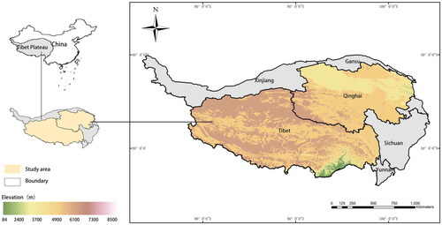
The dominant land cover types are grassland and forest, which account for more than 75% of the land area, and cropland occupies nearly 1%, mainly distributed in the north-eastern edge (Jiang et al. 2020). Wheat and barley are the major crops, contributing to about 60% of the total sown area, which is planted in early April and harvested in September (Di et al. 2021). As the altitude of cropland varies, the crop phenology would be influenced by different climatic conditions, leading to notable variations.

2.2. Data

2.2.1. Remote sensing data and pre-processing

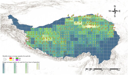
In this study, during the period from June to September in 2022, a 10-m wall-to-wall dataset was created based on Sentinel 2 A and 2B Level-1C top of atmosphere (TOA) reflectance products with cloud-cover less than 20%. In the end, a total of 2360 images were collected from the Sentinel Hub (https://apps.sentinel-hub.com/) (Figure 2).

Figure 2. Acquisition of sentinel 2 images for TP from June to September 2022.

The Sen2Cor module was utilized for atmosphere correction to acquire surface reflectance product (Level-2A) (Main-Knorn et al. 2017), which was adopted to gather training/validating samples for constructing/testing the optimal identification feature knowledge graph of cropland (C_OIFKG) (Zhao et al. 2022) by manual visual interpretation (Table 1). Furthermore, a scene classification layer (SCL) that included different land cover categories such as clouds, cloud shadows, vegetation, water, and bare soils, was also generated by the Sen2Cor module.

Table 1. Sentinel-2 Sensor characteristics.

Band	Central wavelength (nm)	Original spatial resolution (m)
Blue (B)	496.6	10
Green (G)	560.0	10
Red (R)	664.5	10
Red edge 1 (Re1)	703.9	20
Red edge 2 (Re2)	740.2	20
Red edge 3 (Re3)	782.5	20
Near infrared (NIR)	864.8	20
Short-wave infrared 1 (SWIR1)	1613.7	20
Short-wave infrared 2 (SWIR2)	2202.4	20

Two vegetation indicators, the normalized difference water index (NDWI) and land surface water index (LSWI), which are sensitive to leaf water and soil moisture, are also used to identify the unique characteristic of cropland. The two indicators are calculated by following equations (Chen et al. 2005; Xiao et al. 2005): $$\begin{array}{c}\mathit{\text{NDWI}}=\frac{\mathit{\text{NIR}}-\mathit{\text{SWIR}}2}{\mathit{\text{NIR}}+\mathit{\text{SWIR}}2}\end{array}$$ $$\begin{array}{c}\mathit{\text{LSWI}}=\frac{\mathit{\text{NIR}}-\mathit{\text{SWIR}}1}{\mathit{\text{NIR}}+\mathit{\text{SWIR}}1}\end{array}$$

2.2.2. Training and validation data

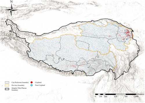
In this study, a total of 10,000 data points were randomly distributed across the entire T&Q. Subsequently, these data points were assessed to ascertain their classification as either homogeneous cropland or non-cropland areas by manual visual interpretation based on Google Earth’s high-resolution imagery since 2020. Additionally, special attention was given to ensuring that the data points were situated at the central regions of the plots (larger than 100 m × 100 m). Finally, after heterogeneous samples were removed, a total of 5702 samples (723 cropland samples versus 4979 non-cropland samples) were used to generate a knowledge-base for further analysis (Figure 3).

Figure 3. The distribution of training samples.

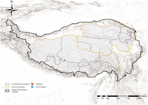
The validation samples in this study were collected using a similar approach as described above, employing an independent accuracy assessment team. A comprehensive dataset comprising a total of 1160 samples (Figure 4), consisting of 310 cropland samples and 850 non-cropland samples, was utilized to construct accurate error matrices, which served as a basis for evaluating the performance and reliability of the identification.

Figure 4. The distribution of validation samples.

2.2.3. Other data

Other auxiliary data used in this study mainly included administrative boundaries, official statistics of cropland area for each city in Tibet Autonomous Region and Qinghai Province, as well as the published cropland maps (one class of land cover products) (Chen et al. 2015; Zhang et al. 2020).

3. Methods

According to the spectral reflectance properties of various land cover types, each land cover exhibits distinct reflection and absorption features at different wavelengths of electromagnetic waves, thereby generating its own unique spectral reflectance curves. As a result, within any given feature space, various land cover types have their own unique distribution patterns, and there must be a theoretical optimal separating hyperplane between different land cover types.

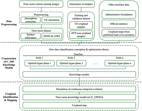
The significant difference of cropland compared to other land cover types is manifested by its distinctive temporal characteristics of human-induced vegetation disturbance throughout the crop growth period. Therefore, to ensure the applicability of cropland identification features, effectively applying them to images captured at any time (day) during the entire crop growth cycle, a time-continuous cropland optimal identification feature model was developed in this study. That is, firstly, a set of optimal identification feature model parameters for each individual period is constructed based on multi-temporal discrete images within the crop growth cycle. Then, these parameters of are temporal reconstructed to establish a knowledge graph of cropland optimal identification feature throughout the crop growth cycle. The workflow of this study with detailed processing steps was presented in Figure 5.

Figure 5. Technical flowchart of this study.

3.1. Construction of cropland optimal identification feature

The determination of optimal identification feature relies on the search for an optimal hyperplane in the given feature space to effectively separate cropland and non-cropland. The optimal hyperplane precisely captures the inherent spatial distribution of the cropland and non-cropland within the feature space, enabling the classification of instances based on their respective distances to the hyperplane. To provide a more generalized approach, the distance was proposed to be transformed into a range between 0 and 1 with a suitable mathematical function, thereby representing the probability of the input instance belonging to the cropland. This probability, defined as the optimal identification feature of cropland (C_OIF), is obtained from the optimal hyperplane and is specific to the cropland, exhibiting definitive cropland-indicative properties. The mathematical expression of the proposed optimal hyperplane is crucial for C_OIF, which is simulated with the logistic regression model in this study.

To consider a feature space dataset $X=\left[x_1,x_2,\dots ,x_n\right]$ and corresponding binary labels $Y=\left[0,1\right].$ The ordinary linear regression prediction model can be expressed as follow: $$\begin{array}{c}Z={\theta }^{T}x={\theta }_0+{\theta }_1{x}_1{+\theta }_2{x}_2+\dots +{\theta }_n{x}_n\end{array}$$

The sigmoid function is utilized by the logistic regression prediction to transform the original value range to the interval [0,1], indicating the probability of the outcome being 1. $$\begin{array}{c}g\left(Z\right)=1+e^{-z}\end{array}$$ $$\begin{array}{c}h\theta \left(X\right)=g\left(X\theta \right)=1+e^{-X\theta }\end{array}$$

When the logistic regression model’s value exceeds the threshold, it is assigned to cropland (1), while values below the threshold are assigned to non-cropland (0), thus accomplishing binary classification. As the $h\theta \left(X\right)$ the function represents the probability of the outcome being 1, the probabilities of classification results being 1 and 0 for any given X are respectively expressed as follows: $$\begin{array}{c}P\left(y=1\right|x,\theta )=h\theta (x)\end{array}$$ $$\begin{array}{c}P\left(y=0\right|x,\theta )=1-h\theta (x)\end{array}$$

Based on the above analysis, the C_OIF model can be defined as follows: $$\begin{array}{c}{C}_{\mathit{\text{OIF}}}=\frac{1}{1+e^{-\left({\theta }_1{x}_1{+\theta }_2{x}_2+\cdots +{\theta }_n{x}_n\right)}}\end{array}$$ where $x_i$ denotes the i-th feature variable in the given feature space, and ${\theta }_i$ denotes the corresponding weight. The weight vector represents the C_OIF model parameters in this study, which encapsulates the optimal segmentation hyperplane of feature space in distinguishing the cropland.

3.2. Generation of cropland optimal identification feature knowledge graph

Due to the growth of crops, the C_OIF exhibit dynamic variations within a growing season. Consequently, C_OIF derived at a particular time (day) may not remain optimal or effective at different time (day), particularly when considering significant temporal intervals. To ensure the applicability of C_OIF at any given time (day) within the crop growth cycle, it is indispensable to develop a daily time-continuous knowledge graph of C_OIF (C_OIFKG). According to factors such as satellite revisit cycles, observation plans, and weather conditions (such as cloud contamination), only discrete daily C_OIF can be acquired using medium/high-resolution remote sensing imagery in most situations. In this study, to generate the C_OIFKG within the crop growth cycle, the linear interpolation is performed on discrete daily C_OIF firstly. Subsequently, a Savitzky-Golay (S-G) filtering method (Savitzky and Golay 1964; Savitzky 1989) is adopted to reconstruct the continuous and smooth C_OIFKG. The S-G filtering window width is set to 15 d, and a second-order polynomial model is selected for smoothing purposes.

3.3. Accuracy assessment

Confusion matrices were generated using the validation samples to assess the overall accuracy (OA), producer’s accuracy (PA, %), user’s accuracy (UA, %), and the Kappa coefficient (Congalton 1991), which were calculated as following equations: $$\begin{array}{c}\mathit{\text{OA}}=\frac{S_d}{n}\times 100\%\end{array}$$ $$\begin{array}{c}\mathit{\text{UA}}=\frac{X_{\mathit{\text{ij}}}}{X_j}\times 100\%\end{array}$$ $$\begin{array}{c}\mathit{\text{PA}}=\frac{X_{\mathit{\text{ij}}}}{X_i}\times 100\%\end{array}$$ $$\begin{array}{c}\mathit{\text{Kappa}}=\frac{\frac{\sum _i{X}_{\mathit{\text{ii}}}}{\sum _{i,j}{X}_{\mathit{\text{ij}}}}-\frac{\sum _i\left(\sum X_{i\mathrm{*}}\times \sum X_{\mathrm{*}i}\right)}{{\left(\sum X_{\mathit{\text{ij}}}\right)}^2}}{1-\frac{\sum _i\left(\sum X_{i\mathrm{*}}\times \sum X_{\mathrm{*}i}\right)}{{\left(\sum X_{\mathit{\text{ij}}}\right)}^2}}\end{array}$$ where $S_d$ is the total number of correctly-identified samples, n denotes the total number of validation samples, $X_{\mathit{\text{ij}}}$ denotes observation in row i column j; $X_i$ denotes the marginal total of row i; $X_j$ denotes the marginal total of column j.

4. Results

4.1. Assessment of cropland identification accuracy

Based on the independent validation samples, the accuracies of cropland distribution of T&Q derived from this was tested. For the entire T&Q, the overall accuracy was 96.6% with the producer’s accuracy of 98.1% and the user’s accuracy of 89.9% for the cropland class, and the Kappa coefficient was 0.9144 (Table 2). It was evident that there was a relatively higher rate of omission errors compared to commission errors in relation to cropland identification. This discrepancy could be primarily attributed to the similarity in land cover and management practices between cropland and pasturelands (artificially managed grasslands), which led to exhibit patterns and characteristics confused with cropland, posed challenges for accurate differentiation.

Table 2. Assessment of cropland distribution of T&Q with independent validation samples.

	Non-Cropland	Cropland	Total	UA (%)
Non-Cropland	816	6	822	99.3
Cropland	34	304	338	89.9
Total	850	310	1160
PA (%)	96.0	98.1
OA (%)	96.6
Kappa	0.9144

4.2. Cropland acreage estimation of T&Q in 2022

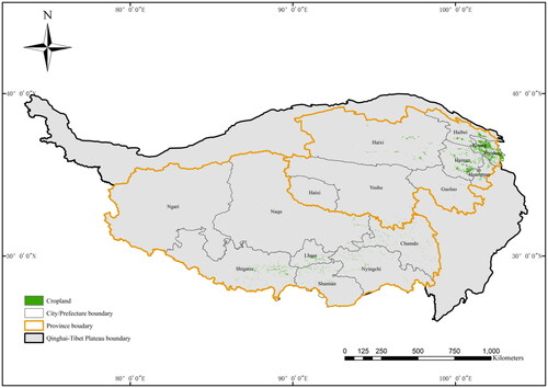
The spatial distribution of cropland of T&Q in 2022 is shown in Figure 6. In the entire region of T&Q, the total cropland acreage was estimated at 1,800,160 hectares, which accounted for about 1% of the total land area, and the majority of croplands are primarily concentrated in the northeastern of Qinghai province, accounting for approximately 2/3 of the total cropland within T&Q. The cropland acreage in Qinghai Province is approximately 2.5 times larger than that in Tibet Autonomous Region. Nearly 75% of croplands within Qinghai Province are distributed in Haidong, Hainan Prefecture and Xining. In the Tibet Autonomous Region, most of the croplands (68.5%) are concentrated in Lhasa, Shigatse and Chamdo, and the quantity of croplands in Nyingchi and Shannan exhibits a similar magnitude, constituting approximately 25% of the total.

Figure 6. The Spatial distribution of cropland of T&Q in 2022.

Considering the elevation, the croplands of T&Q are mainly distributed in the range of 2000–4000 m, constituting approximately 88.6% of the total cropland. Notably, a significant portion of the croplands, around 46.11%, is concentrated specifically within the elevation range of 3000–4000 m. The subsequent elevation range of 4000–5000 m comprises approximately 10.0%. At elevations exceeding 5000 m, the distribution of cropland is scarce, due to extremely limited agricultural activities in these high-altitude areas.

5. Discussion

5.1. Comparison with other released datasets

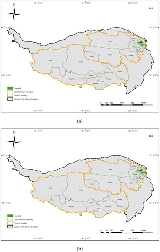
Cropland layers from two released land cover datasets (Chen et al. 2015; Zhang et al. 2020) in 2020 was collected to compare with the result of this study. Compared to the cropland map of Zhang et al. (2020), the monitoring results of this study demonstrate a higher level of concurrence with that of Chen et al. (2015). In the cropland distribution presented in Zhang et al. (2020) (Figure 7b), there is an evident underestimation of cropland in the Tibet Autonomous Region, especially in Lhasa, Shigatse and Nyingchi, where the croplands had a dendritic distribution along rivers. This discrepancy can be mainly attributed to the region’s high elevations, intricate topography, and fragmented parcels of cropland, which collectively pose challenges to accurate identification.

Figure 7. The spatial distribution of two released land cover datasets in 2020. (a) cropland layer derived from (Chen et al. 2015); (b) cropland layer derived from (Zhang et al. 2020).

The total cropland acreage of T&Q estimated in this study lies within the range of estimates provided by the two released land cover datasets, which is 3.56% lower than (Chen et al. 2015) and 16.4% higher than (Zhang et al. 2020). In comparison to the cropland acreage estimation at city/prefecture level (Figure 8), the estimations from this study for regions with concentrated cropland areas, including Xining, Haidong, and Hainan Prefecture in Qinghai Province, as well as Lhasa, Shigatse, and Chamdo in the Tibet Autonomous Region, are relatively consistent with the estimates derived from (Chen et al. 2015). Except for Hainan Prefecture (44.3%) and Shigatse (21.8%), the deviations of cropland acreage estimate for other cities/prefectures mentioned above are within 11%. The estimates obtained by Zhang et al. (2020) show relatively smaller deviations within 9% for regions such as Xining, Haidong, and Hainan Prefecture in Qinghai Province when compared to the results of this study. Nevertheless, substantial disparities between the estimates from (Zhang et al. 2020) and this study are apparent in cities/prefectures within the Tibet Autonomous Region, including Lhasa, Shigatse, and Chamdo, with deviations exceeding 40% and certain cities/prefectures (Lhasa and Chamdo) exhibiting deviations of more than 10 times. These disparities may arise due to discrepancies in the definition of cropland in the two land cover datasets, which were not the primary focus on cropland identification.

Figure 8. The cropland acreage estimation at the municipal/prefectural level of T&Q in 2022.

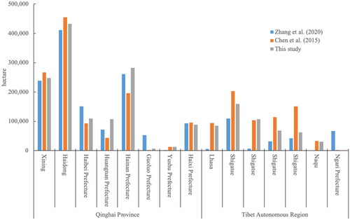
In regions with sparse and scattered cropland distribution, such as Yushu Prefecture in Qinghai Province and Naqu, Ngari Prefecture, and Nyingchi in the Tibet Autonomous Region, significant disparities are observed between the cropland estimations of this study and those derived from (Zhang et al. 2020). Moreover, variations are evident between the cropland estimations of this study and those of Chen et al. (2015) for regions including Huangnan Prefecture and Guoluo Prefecture in Qinghai Province, as well as Ngari Prefecture in the Tibet Autonomous Region. The identification of dispersed cropland in specific regions poses persistent challenges, moreover, with the expanding of the monitoring area, there is a tendency to inadvertently neglect the monitoring accuracy of these regions.

5.2. Comparison with regional statistical data

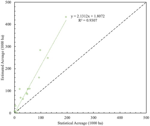
By comparing the municipal/prefectural-level cropland acreage statistics collected from the statistical yearbook of Qinghai Provincial Bureau of Statistics and NBS Survey Office in Qinghai (2020) and Tibet Autonomous Region Bureau of Statistics and NBS Survey Office in Tibet (2019) with the monitoring results of this study, it had been observed that consistent trends were generally exhibited (Figure 9). However, the estimated cropland acreage in this study tends to be obviously overestimated in comparison to the statistics. Although the temporal inconsistency between the monitoring results (2022) and the statistical data (2020) may introduce certain errors, this is primarily attributed to the misclassification of land cover types such as pastures as cropland. Additionally, the disparity between the data acquisition year of the statistics and the monitoring year of this study may introduce certain errors. Moreover, it is worth noting that in regions where cropland was smaller and more scattered, there is a more significant discrepancy between the estimated results of this study and the municipal/prefectural-level statistics. The relative errors in some municipalities/prefectures exceed 200%, indicating that more refined remote sensing imagery or the selection of more suitable identification features is required for cropland identification in these regions.

Figure 9. Consistency of estimated acreage and statistical acreage at the municipal/prefectural level.

5.3. Advantages and limitations

In most current studies on land cover identification with remote sensing, there was a pronounced trend of high integration and interdependency between identification features and methods. Moreover, a strong reliance on both labeled training sample data and empirical knowledge was also exhibited. In this study, to address this issue, by integrating sample data and satellite imageries to drive machine learning models, C_OIFKG was developed based on the feature distribution patterns and regularities derived from the original data. The utilization of C_OIFKG enhanced the separability between cropland and non-cropland, thereby reducing the dependency of the classification process on labeled training samples data. Additionally, C_OIFKG, which was independent of the inter-annual variations of cropland, developed a robust understanding of the cropland characteristics and exhibit improved potential generalization performance on cropland identification even in years with different planting conditions.

Furthermore, C_OIFKG only required one image within a single growing season to complete cropland distribution mapping, and the acquisition times of images from different locations can be different. Because C_OIFKG was constructed based on discrete knowledge models using interpolation and smoothing strategies, it can generate a C_OIF on any given day within a year. Therefore, it has significant advantages in generating cropland distribution maps, particularly in regions with limited cloud-free imagery or short crop growing seasons.

However, there were also limitations for the C_OIFKG approach. Firstly, the construction of C_OIFKG is based on extensive data processing. In order to reconstruct the C_OIFKG for the entire T&Q region, a total of 11,904 images from June to September in 2022, as long as the training samples were not cloud-covered, were collected and processed in this study. With the rapid development of high-performance data process technology, such as cloud computing, this would be expected to be further mitigated. Secondly, the investigation of C_OIFKG construction was solely based on Sentinel-2 data in this study, but considering the significance of C_OIFKG, more remote sensing data used in C_OIFKG reconstructing would enhance the universality of its application, consequently, the assimilation and fusion of multi-source remote sensing data clearly emerged as subsequent issues worthy of attention. Thirdly, in new regions with different crop types, phenological stages, crop rotation systems, it is necessary to reconstruct the suitable C_OIFKG to ensure the cropland identification accuracy for specific region.

The accuracy assessment methods for existing remote sensing monitoring products primarily rely on conventional metrics such as OA, PA, UA, Kappa, etc. However, these metrics are often useless, misleading and/or flawed for many practical remote sensing applications (Pontius and Millones 2011). Consequently, with the current proliferation of various remote sensing monitoring products, there is an urgent need to expand new accuracy assessment metrics to ensure more objective and practical evaluations aligned with real-world applications.

6. Conclusions

In this study, the feasibility of cropland extraction based on optimal identification feature knowledge graph without the requirement of labeled samples to train the classifier has been demonstrated, which will improve the timeliness and automation level of remote sensing based regional cropland mapping. C_OIFKG demonstrated improved potential generalization performance on cropland identification in years with different planting conditions. At a minimum, C_OIFKG requires only one image per growing season for complete cropland distribution mapping, with acquisition times varying across different locations. Even in the T&Q region where cropland is not prevalent, the method proposed in this study still achieved promising performance in cropland identification. The overall accuracy was 96.6% with the producer’s accuracy of 98.1% and the user’s accuracy of 89.9% for the cropland class, and the Kappa coefficient was 0.9144. Most of the croplands (approximately 88.6%) in the T&Q region are mainly distributed in the elevation range of 2000–4000 m, where the agricultural ecosystem is highly vulnerable and agricultural activities are confronted with considerable difficulties. Therefore, the prompt and precise acquisition cropland dynamics information in the T&Q region holds evident significance for regional food security and sustainable agricultural development. For further study, the C_OIFKG approach should be implemented across different years in the T&Q region or over other regions with different cropping systems and phenology patterns based on multi-source remote sensing data.

Authors contributions

Conceptualization, Xin Du, Qiangzi Li and Longcai Zhao; Methodology, Xin Du and Longcai Zhao; Validation, Xin Du, Yunqi Shen, Sichen Zhang and Jingyuan Xu; Writing—original draft preparation, Xin Du; Writing—review and editing, Qiangzi Li, Longcai Zhao, Yuan Zhang, Hongyan Wang; Supervision, Qiangzi Li; Project administration, Xin Du. All authors have read and agreed to the published version of the manuscript.

Data availability statement

The data that support the findings of this study are available from the corresponding author upon reasonable requests.

Disclosure statement

No potential conflict of interest was reported by the author(s).

Additional information

Funding

This study was funded by the National Key R&D Program of China (2021YFE0117800) and the Key Program of High-resolution Earth Observation System (00-Y30B01-9001-22/23-CY-10, 20-Y30F10-9001-20/22).

References

- Alcantara C, Kuemmerle T, Prishchepov AV, Radeloff VC. 2012. Mapping abandoned agriculture with multi-temporal MODIS satellite data. Remote Sens Environ. 124:334–347. doi: 10.1016/j.rse.2012.05.019.
- Buttner G. 2014. CORINE land cover and land cover change products. In: Manakos, I., Braun, M. (eds). Land Use and Land Cover Mapping in Europe. Remote Sensing and Digital Image Processing, vol 18. Dordrecht: Springer Netherlands.
- Chen A, Huang L, Liu Q, Piao S. 2021. Optimal temperature of vegetation productivity and its linkage with climate and elevation on the Tibetan Plateau. Glob Chang Biol. 27(9):1942–1951. doi: 10.1111/gcb.15542.
- Chen D, Huang J, Jackson TJ. 2005. Vegetation water content estimation for corn and soybeans using spectral indices derived from MODIS near- and short-wave infrared bands. Remote Sens Environ. 98(2-3):225–236. doi: 10.1016/j.rse.2005.07.008.
- Chen J, Chen J, Liao A, Cao X, Chen L, Chen X, He C, Han G, Peng S, Lu M, et al. 2015. Global land cover mapping at 30m resolution: a POK-based operational approach. ISPRS J Photogramm Remote Sens. 103:7–27. doi: 10.1016/j.isprsjprs.2014.09.002.
- Congalton RG. 1991. A review of assessing the accuracy of classifications of remotely sensed data. Remote Sens Environ. 37(1):35–46. doi: 10.1016/0034-4257(91)90048-B.
- Di Y, Zhang G, You N, Yang T, Zhang Q, Liu R, Doughty RB, Zhang Y. 2021. Mapping croplands in the granary of the Tibetan plateau using all available Landsat imagery, a phenology-based approach, and google earth engine. Remote Sensing. 13(12):2289. doi: 10.3390/rs13122289.
- Dong J, Xiao X, Kou W, Qin Y, Zhang G, Li L, Jin C, Zhou Y, Wang J, Biradar C, et al. 2015. Tracking the dynamics of paddy rice planting area in 1986–2010 through time series Landsat images and phenology-based algorithms. Remote Sens Environ. 160:99–113. doi: 10.1016/j.rse.2015.01.004.
- Egorov AV, Hansen MC, Roy DP, Kommareddy A, Potapov PV. 2015. Image interpretation-guided supervised classification using nested segmentation. Remote Sens Environ. 165:135–147. doi: 10.1016/j.rse.2015.04.022.
- Estel S, Kuemmerle T, Alcántara C, Levers C, Prishchepov A, Hostert P. 2015. Mapping farmland abandonment and recultivation across Europe using MODIS NDVI time series. Remote Sens Environ. 163:312–325. doi: 10.1016/j.rse.2015.03.028.
- Friedl MA, Sulla-Menashe D, Tan B, Schneider A, Ramankutty N, Sibley A, Huang X. 2010. MODIS Collection 5 global land cover: algorithm refinements and characterization of new datasets. Remote Sens Environ. 114(1):168–182. doi: 10.1016/j.rse.2009.08.016.
- Fritz S, See L, McCallum I, Schill C, Obersteiner M, Van Der Velde M, Boettcher H, Havlík P, Achard F. 2011. Highlighting continued uncertainty in global land cover maps for the user community. Environ Res Lett. 6(4):044005. doi: 10.1088/1748-9326/6/4/044005.
- Gallego FJ, Kussul N, Skakun S, Kravchenko O, Shelestov A, Kussul O. 2014. Efficiency assessment of using satellite data for crop area estimation in Ukraine. Int J Appl Earth Obs Geoinf. 29:22–30. doi: 10.1016/j.jag.2013.12.013.
- Hegazy IR, Kaloop MR. 2015. Monitoring urban growth and land use change detection with GIS and remote sensing techniques in Daqahlia governorate Egypt. Int J Sustain Built Environ. 4(1):117–124. doi: 10.1016/j.ijsbe.2015.02.005.
- Jeganathan C, Dash J, Atkinson PM. 2014. Remotely sensed trends in the phenology of northern high latitude terrestrial vegetation, controlling for land cover change and vegetation type. Remote Sens Environ. 143:154–170. doi: 10.1016/j.rse.2013.11.020.
- Jiang W, Lü Y, Liu Y, Gao W. 2020. Ecosystem service value of the Qinghai-Tibet Plateau significantly increased during 25 years. Ecosyst Serv. 44:101146. doi: 10.1016/j.ecoser.2020.101146.
- Khan S, Tufail M, Khan MT, Khan ZA, Anwar S. 2021. Deep learning-based identification system of weeds and crops in strawberry and pea fields for a precision agriculture sprayer. Precision Agric. 22(6):1711–1727. doi: 10.1007/s11119-021-09808-9.
- Lary DJ, Alavi AH, Gandomi AH, Walker AL. 2016. Machine learning in geosciences and remote sensing. Geosci Front. 7(1):3–10. doi: 10.1016/j.gsf.2015.07.003.
- Main-Knorn M, Pflug B, Louis J, Debaecker V, Gascon F. 2017. Sen2Cor for Sentinel-2. In: Image & Signal Processing for Remote Sensing.
- Mountrakis G, Im J, Ogole C. 2011. Support vector machines in remote sensing: a review. ISPRS J Photogramm Remote Sens. 66(3):247–259. doi: 10.1016/j.isprsjprs.2010.11.001.
- Pontius RG, Millones M. 2011. Death to Kappa: birth of quantity disagreement and allocation disagreement for accuracy assessment. Int J Remote Sens. 32(15):4407–4429. doi: 10.1080/01431161.2011.552923.
- Qinghai Provincial Bureau of Statistics and NBS Survey Office in Qinghai. 2020. Qinghai statistical yearbook. China Statistics Press.
- Savitzky A, Golay M. 1964. Smoothing and differentiation of data by simplified least squares procedures. Anal Chem. 36(8):1627–1639. doi: 10.1021/ac60214a047.
- Savitzky A. 1989. A historic collaboration. Anal Chem. 61(15):921A–923A. doi: 10.1021/ac00190a744.
- Teluguntla P, Thenkabail PS, Oliphant A, Xiong J, Gumma MK, Congalton RG, Yadav K, Huete A. 2018. A 30-m landsat-derived cropland extent product of Australia and China using random forest machine learning algorithm on Google Earth Engine cloud computing platform. ISPRS J Photogramm Remote Sens. 144:325–340. doi: 10.1016/j.isprsjprs.2018.07.017.
- Teluguntla P, Thenkabail PS, Xiong J, Gumma MK, Congalton RG, Oliphant A, Poehnelt J, Yadav K, Rao M, Massey R. 2017. Spectral matching techniques (SMTs) and automated cropland classification algorithms (ACCAs) for mapping croplands of Australia using MODIS 250-m time-series (2000–2015) data. Int J Digital Earth. 10(9):944–977. doi: 10.1080/17538947.2016.1267269.
- Thenkabail PS, Wu Z. 2012. An automated cropland classification algorithm (ACCA) for Tajikistan by combining Landsat, MODIS, and secondary data. Remote Sens. 4(10):2890–2918. doi: 10.3390/rs4102890.
- Tibet Autonomous Region Bureau of Statistics and NBS Survey Office in Tibet. 2020. Tibet statistical yearbook. China Statistics Press.
- Tseng M-H, Chen S-J, Hwang G-H, Shen M-Y. 2008. A genetic algorithm rule-based approach for land-cover classification. ISPRS J Photogramm Remote Sens. 63(2):202–212. doi: 10.1016/j.isprsjprs.2007.09.001.
- Wang C, Gao Q, Yu M. 2019. Quantifying trends of land change in Qinghai-Tibet Plateau during 2001–2015. Remote Sensing. 11(20):2435. doi: 10.3390/rs11202435.
- Wang X, He K, Dong Z. 2019. Effects of climate change and human activities on runoff in the Beichuan River Basin in the northeastern Tibetan Plateau, China. CATENA. 176:81–93. doi: 10.1016/j.catena.2019.01.001.
- Xiao X, Boles S, Liu J, Zhuang D, Frolking S, Li C, Salas W, Moore B. 2005. Mapping paddy rice agriculture in southern China using multi-temporal MODIS images. Remote Sens Environ. 95(4):480–492. doi: 10.1016/j.rse.2004.12.009.
- Xie D, Xu H, Xiong X, Liu M, Hu H, Xiong M, Liu L. 2023. Cropland extraction in Southern China from very high-resolution images based on deep learning. Remote Sensing. 15(9):2231. doi: 10.3390/rs15092231.
- Xiong J, Thenkabail P, Tilton J, Gumma M, Teluguntla P, Oliphant A, Congalton R, Yadav K, Gorelick N. 2017a. Nominal 30-m cropland extent map of continental Africa by integrating pixel-based and object-based algorithms using Sentinel-2 and Landsat-8 data on google earth engine. Remote Sens. 9(10):1065. doi: 10.3390/rs9101065.
- Xiong J, Thenkabail PS, Gumma MK, Teluguntla P, Poehnelt J, Congalton RG, Yadav K, Thau D. 2017b. Automated cropland mapping of continental Africa using Google Earth Engine cloud computing. ISPRS J Photogramm Remote Sens. 126:225–244. doi: 10.1016/j.isprsjprs.2017.01.019.
- Xu J, Zhu Y, Zhong R, Lin Z, Xu J, Jiang H, Huang J, Li H, Lin T. 2020. DeepCropMapping: a multi-temporal deep learning approach with improved spatial generalizability for dynamic corn and soybean mapping. Remote Sens Environ. 247:111946. doi: 10.1016/j.rse.2020.111946.
- Yang C, Everitt JH, Murden D. 2011. Evaluating high resolution SPOT 5 satellite imagery for crop identification. Comput Electron Agric. 75(2):347–354. doi: 10.1016/j.compag.2010.12.012.
- Yao T, Thompson L, Yang W, Yu W, Gao Y, Guo X, Yang X, Duan K, Zhao H, Xu B, et al. 2012. Different glacier status with atmospheric circulations in Tibetan Plateau and surroundings. Nature Clim Change. 2(9):663–667. doi: 10.1038/nclimate1580.
- Zhang G, Dong J, Zhou C, Xu X, Wang M, Ouyang H, Xiao X. 2013. Increasing cropping intensity in response to climate warming in Tibetan Plateau, China. Field Crops Research. 142:36–46. doi: 10.1016/j.fcr.2012.11.021.
- Zhang X, Liu L, Wu C, Chen X, Gao Y, Xie S, Zhang B. 2020. Development of a global 30 m impervious surface map using multisource and multitemporal remote sensing datasets with the Google Earth Engine platform. Earth Syst Sci Data. 12(3):1625–1648., doi: 10.5194/essd-12-1625-2020.
- Zhao L, Li Q, Chang Q, Shang J, Du X, Liu J, Dong T. 2022. In-season crop type identification using optimal feature knowledge graph. ISPRS J Photogramm Remote Sens. 194:250–266. doi: 10.1016/j.isprsjprs.2022.10.017.