Generalized discrete and ultradiscrete Burgers equations derived through the correlated random walk

Abstract

The correlated random walk is known as a generalization of the well-known random walk. In this study, we present that a generalized discrete Burgers equation corresponding to the correlated random walk can be obtained through a Cole–Hopf transformation to a generalized discrete diffusion equation. By applying a technique called ultradiscretization, the generalized ultradiscrete diffusion equation, the ultradiscrete Cole–Hopf transformation, and a variant of the ultradiscrete Burgers equation are obtained. Additionally, this study shows that the resulting ultradiscrete Burgers equation yields cellular automata that can be interpreted as a traffic flow model with controllability of vehicle flow.

Keywords:

• Discrete Burgers equation
• correlated random walk
• Cole–Hopf transformation
• cellular automata
• traffic flow model

AMS:

• 39A60
• 82C41
• 37J70
• 37B15

1. Introduction

The elementary cellular automata (CA) of rule 184 is a well-known fundamental traffic flow model. Nishinari and Takahashi [10] found that the elementary CA of rule 184 is related to the discrete Burgers equation (1) $u_j^{n+1}=u_j^n\frac{u_{j+1}^n+1/u_j^n}{u_j^n+1/u_{j-1}^n},$(1) through the limiting procedure called the ultradiscretization [12] in the context of integrable systems. That is, the ultradiscretization of the discrete Burgers equation (1(1) $u_j^{n+1}=u_j^n\frac{u_{j+1}^n+1/u_j^n}{u_j^n+1/u_{j-1}^n},$(1) ) yields the ultradiscrete Burgers equation (2) $U_j^{n+1}=U_j^n+min(U_{j-1}^n,L-U_j^n,)-min(U_j^n,L-U_{j+1}^n),$(2) where j and n are discrete spacial and time variables, respectively. Here, the ultradiscretization is based on the formula $\underset{\epsilon \to +0}{lim}\epsilon \log ({\mathrm{e}}^{a/\epsilon }+{\mathrm{e}}^{b/\epsilon })=max(a,b)$for $a,b\in \mathbb{R}$. If L = 1 and $U_j^n\in \{0,1\}$ are set in (2(2) $U_j^{n+1}=U_j^n+min(U_{j-1}^n,L-U_j^n,)-min(U_j^n,L-U_{j+1}^n),$(2) ), then the dynamics of (2(2) $U_j^{n+1}=U_j^n+min(U_{j-1}^n,L-U_j^n,)-min(U_j^n,L-U_{j+1}^n),$(2) ) are exactly the same as the elementary CA rule 184 [10]. Some generalizations, interpretation as traffic flow, and their mathematical analyses, which originate from this model, are studied in [2,3].

Taking a continuous limit of the discrete Burgers equation, the well-known (continuous) Burgers equation is obtained. Despite its nonlinearity, the Burgers equation can be transformed into linear diffusion equation through a variable transformation called the Cole–Hoph transformation [1,6]. Because of the Cole–Hoph transformation, the exact solutions can be obtained for the Burgers equation. 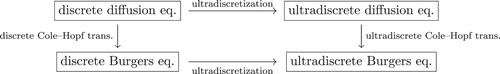Similarly, for discrete equations, the discrete Burgers equation (1(1) $u_j^{n+1}=u_j^n\frac{u_{j+1}^n+1/u_j^n}{u_j^n+1/u_{j-1}^n},$(1) ) transformed into the discrete diffusion equation (3) $f_j^{n+1}=\frac{1}{2}(f_{j+1}^n+f_{j-1}^n)$(3) through the discrete Cole–Hopf transformation (4) $u_j^n=\frac{f_{j+1}^n}{f_j^n},$(4) which is shown in [5]. The relation of these equations is summarized in Figure 1.

Figure 1. Diagram of four equations: the discrete diffusion equation (3(3) $f_j^{n+1}=\frac{1}{2}(f_{j+1}^n+f_{j-1}^n)$(3) ), discrete Burgers equation (1(1) $u_j^{n+1}=u_j^n\frac{u_{j+1}^n+1/u_j^n}{u_j^n+1/u_{j-1}^n},$(1) ) ultradiscrete diffusion equation and ultradiscrete Burgers equation (2(2) $U_j^{n+1}=U_j^n+min(U_{j-1}^n,L-U_j^n,)-min(U_j^n,L-U_{j+1}^n),$(2) ).

If $f_j^n$ is regarded as existence probability of particles at site j and discrete time n, the discrete diffusion equation (3(3) $f_j^{n+1}=\frac{1}{2}(f_{j+1}^n+f_{j-1}^n)$(3) ) is equivalent to the evolution equation of the symmetric (isotropic) random walk on one dimensional lattice over $\mathbb{Z}$. The position of a particle is, of course, a Markov chain.

The correlated random walk is a generalization of the random walk, which depends on the previous position of a particle [8,9,11], which is also known as the persistent random walk or Goldstein-Kac random walk [4,7]. Since the correlated random walk is double stochastic, it is no longer Markov chain. The correlated random walk has the ability to connect the continuous wave equation and heat equation through the telegraph equation [13] because of the non-Markovian. Thus, this study is interested in the effect of discrete and ultradiscrete equations, which is induced by the correlated random walk, on the non-Markovian. However, to the best of the present authors' knowledge, there is currently no literature concerning the relationship between the correlated random walk and discrete or ultradiscrete equations.

The paper discusses the following two aspects: First, the relationship is found to be similar to Figure 1 for the correlated random walk. The key idea, here, is the Cole–Hopf transformations must be considered with respect to not only space but also discrete time. Secondly, the ultradiscrete equation is regarded as a CA that describes dynamics of a traffic flow. The non-Markovian underlying the correlated random walk is inherited by the traffic flow model, in which the movement of cars depends on not only the previous time but also the time before last.

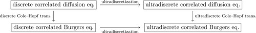
The rest of the paper is organized as follows. Section 2 derives the three-term recurrence relation of the correlated random walk and introduces the appropriate discrete Cole–Hopf transformation to obtain generalized Burgers equations. Section 3 applies the ultradiscretization to the Burgers equations and clarifies the commutativity of the proposed Cole–Hopf transformation and the ultradiscretization for the correlated random walk, meaning that the commutative diagram of the correlated random walk is obtained, which is a generalization of Figure 1 (see Figure 2). Section 4 shows that the ultradiscrete equation derived in Section 3 can be regarded as a CA. Section 5 shows that the CA shown in Section 4 can be regarded as a traffic flow model, which possesses the non-Markovian of the original correlated random walk and discusses the fundamental diagram of the traffic flow model. Finally, Section 6 provides the concluding remarks.

Figure 2. Diagram of four equations: discrete correlated diffusion equation (7(7) $f_j^{n+1}=p(f_{j-1}^n+f_{j+1}^n)-(2p-1)f_j^{n-1}.$(7) ), discrete correlated Burgers equation (9(9) $\{\begin{array}{l}{\displaystyle u_j^{n+1}=u_j^n\cdot \frac{p(u_{j+1}^n+1/u_j^n)-(2p-1)\cdot 1/v_{j+1}^{n-1}}{p(u_j^n+1/u_{j-1}^n)-(2p-1)\cdot 1/v_j^{n-1}},}\\ {\displaystyle v_j^{n+1}=v_j^n\cdot \frac{p(u_j^{n+1}+1/u_{j-1}^{n+1})-(2p-1)\cdot 1/v_j^n}{p(u_j^n+1/u_{j-1}^n)-(2p-1)\cdot 1/v_j^{n-1}}.}\end{array}$(9) ) ultradiscrete correlated diffusion equation (11(11) $F_j^{n+1}=max(F_{j-1}^n,F_{j+1}^n,R+F_j^{n-1}),R>-\mathrm{\infty }.$(11) ), and ultradiscrete correlated Burgers equation (14(14) $\{\begin{array}{l}{U}_j^{n+1}=U_j^n+min(U_{j-1}^n,L-U_j^n,V_j^{n-1}-R)-min(U_j^n,L-U_{j+1}^n,V_{j+1}^{n-1}-R),\\ V_j^{n+1}=V_j^n+min(U_{j-1}^n,L-U_j^n,V_j^{n-1}-R)-min(U_{j-1}^{n+1},L-U_j^{n+1},V_j^n-R).\end{array}$(14) ).

2. Discrete diffusion equation induced by a correlated random walk and its discrete Cole–Hopf transformation

Consider the random walk model on the one-dimensional lattice in which a particle moves the left and right neighbours with probabilities 1/2 and 1/2 respectively. The discrete diffusion equation (3(3) $f_j^{n+1}=\frac{1}{2}(f_{j+1}^n+f_{j-1}^n)$(3) ) is nothing but the time evolution of this random walk; that is, $f_j^n$ corresponds to the finding probability at discrete time n and position j.

Next consider the correlated random walk on the one-dimensional lattice which is a generalization of the above random walk. In the correlated random walk, the probabilities of a particle at each position associated with moving left and right are determined by the directions from which a particle comes into the position. Then let ${\mu }_L^n(j)$ and ${\mu }_R^n(j)$ be the probabilities that a particle moves to the position j from the positions j + 1 and j−1 at discrete time n, respectively. The time evolution of the correlated random walk with parameters $p,q\in [0,1]$ is denoted by (5) $\{\begin{array}{l}{\mu }_L^{n+1}(j)=p{\mu }_L^n(j+1)+(1-q){\mu }_R^n(j+1),\\ {\mu }_R^{n+1}(j)=(1-p){\mu }_L^n(j-1)+q{\mu }_R^n(j-1).\end{array}$(5) Here, the parameter p (resp. q) is the probability that the leftward (resp. rightward) movement is repeated twice in a row, respectively. Note that if $p=q=1/2$, then the discrete diffusion equation (3(3) $f_j^{n+1}=\frac{1}{2}(f_{j+1}^n+f_{j-1}^n)$(3) ) is recovered.

In the following, p = q is set for simplicity, after which the second equation of (5(5) $\{\begin{array}{l}{\mu }_L^{n+1}(j)=p{\mu }_L^n(j+1)+(1-q){\mu }_R^n(j+1),\\ {\mu }_R^{n+1}(j)=(1-p){\mu }_L^n(j-1)+q{\mu }_R^n(j-1).\end{array}$(5) ) is reduced to ${\mu }_L^n(j-1)=\frac{1}{1-p}({\mu }_R^{n+1}(j)-p{\mu }_R^n(j-1)).$Inserting this into the first equation of (5(5) $\{\begin{array}{l}{\mu }_L^{n+1}(j)=p{\mu }_L^n(j+1)+(1-q){\mu }_R^n(j+1),\\ {\mu }_R^{n+1}(j)=(1-p){\mu }_L^n(j-1)+q{\mu }_R^n(j-1).\end{array}$(5) ), we have the following recurrence equation of ${\mu }_R^{(n)}(j)$: (6) $\begin{array}{rl}& \frac{1}{1-p}({\mu }_R^{n+2}(j+1)-p{\mu }_R^{n+1}(j))\\ & =\frac{p}{1-p}({\mu }_R^{n+1}(j+2)-p{\mu }_R^n(j+1))+(1-p){\mu }_R^n(j+1).\end{array}$(6) Through the valiable substitution $f_j^n:={\mu }_R^n(j)$, equation (6(6) $\begin{array}{rl}& \frac{1}{1-p}({\mu }_R^{n+2}(j+1)-p{\mu }_R^{n+1}(j))\\ & =\frac{p}{1-p}({\mu }_R^{n+1}(j+2)-p{\mu }_R^n(j+1))+(1-p){\mu }_R^n(j+1).\end{array}$(6) ) yields $f_{j+1}^{n+2}=p{f}_j^{n+1}+p{f}_{j+2}^{n+1}+\{(1-p{)}^2-p^2\}{f}_{j+1}^n.$Then, the following three-term recurrence equation representing the correlated random walk is obtained: (7) $f_j^{n+1}=p(f_{j-1}^n+f_{j+1}^n)-(2p-1)f_j^{n-1}.$(7) If $p=1/2$, the time evolution of the usual random walk (3(3) $f_j^{n+1}=\frac{1}{2}(f_{j+1}^n+f_{j-1}^n)$(3) ) appears. This study refers to (7(7) $f_j^{n+1}=p(f_{j-1}^n+f_{j+1}^n)-(2p-1)f_j^{n-1}.$(7) ) as the discrete correlated diffusion equation.

Next, apply a discrete Cole–Hopf transformation to the time evolution equation of the correlated random walk (7(7) $f_j^{n+1}=p(f_{j-1}^n+f_{j+1}^n)-(2p-1)f_j^{n-1}.$(7) ). Through a consideration of the usual discrete Cole–Hopf transformation (4(4) $u_j^n=\frac{f_{j+1}^n}{f_j^n},$(4) ) of the random walk (3(3) $f_j^{n+1}=\frac{1}{2}(f_{j+1}^n+f_{j-1}^n)$(3) ), another discrete Cole–Hopf transformation of the correlated random walk is defined by the following pair of the spatial and temporal ratios of the finding probabilities: (8) $u_j^n=\frac{f_{j+1}^n}{f_j^n},v_j^n=\frac{f_j^{n+1}}{f_j^n}.$(8) Then, inserting (7(7) $f_j^{n+1}=p(f_{j-1}^n+f_{j+1}^n)-(2p-1)f_j^{n-1}.$(7) ) into (8(8) $u_j^n=\frac{f_{j+1}^n}{f_j^n},v_j^n=\frac{f_j^{n+1}}{f_j^n}.$(8) ), $u_j^n$ and $v_j^n$ must satisfy the following recursions: (9) $\{\begin{array}{l}{\displaystyle u_j^{n+1}=u_j^n\cdot \frac{p(u_{j+1}^n+1/u_j^n)-(2p-1)\cdot 1/v_{j+1}^{n-1}}{p(u_j^n+1/u_{j-1}^n)-(2p-1)\cdot 1/v_j^{n-1}},}\\ {\displaystyle v_j^{n+1}=v_j^n\cdot \frac{p(u_j^{n+1}+1/u_{j-1}^{n+1})-(2p-1)\cdot 1/v_j^n}{p(u_j^n+1/u_{j-1}^n)-(2p-1)\cdot 1/v_j^{n-1}}.}\end{array}$(9) This study refers to (9(9) $\{\begin{array}{l}{\displaystyle u_j^{n+1}=u_j^n\cdot \frac{p(u_{j+1}^n+1/u_j^n)-(2p-1)\cdot 1/v_{j+1}^{n-1}}{p(u_j^n+1/u_{j-1}^n)-(2p-1)\cdot 1/v_j^{n-1}},}\\ {\displaystyle v_j^{n+1}=v_j^n\cdot \frac{p(u_j^{n+1}+1/u_{j-1}^{n+1})-(2p-1)\cdot 1/v_j^n}{p(u_j^n+1/u_{j-1}^n)-(2p-1)\cdot 1/v_j^{n-1}}.}\end{array}$(9) ) as the discrete correlated Burgers equation. Note that if $p=1/2$ is put into (9(9) $\{\begin{array}{l}{\displaystyle u_j^{n+1}=u_j^n\cdot \frac{p(u_{j+1}^n+1/u_j^n)-(2p-1)\cdot 1/v_{j+1}^{n-1}}{p(u_j^n+1/u_{j-1}^n)-(2p-1)\cdot 1/v_j^{n-1}},}\\ {\displaystyle v_j^{n+1}=v_j^n\cdot \frac{p(u_j^{n+1}+1/u_{j-1}^{n+1})-(2p-1)\cdot 1/v_j^n}{p(u_j^n+1/u_{j-1}^n)-(2p-1)\cdot 1/v_j^{n-1}}.}\end{array}$(9) ), the first equation of (9(9) $\{\begin{array}{l}{\displaystyle u_j^{n+1}=u_j^n\cdot \frac{p(u_{j+1}^n+1/u_j^n)-(2p-1)\cdot 1/v_{j+1}^{n-1}}{p(u_j^n+1/u_{j-1}^n)-(2p-1)\cdot 1/v_j^{n-1}},}\\ {\displaystyle v_j^{n+1}=v_j^n\cdot \frac{p(u_j^{n+1}+1/u_{j-1}^{n+1})-(2p-1)\cdot 1/v_j^n}{p(u_j^n+1/u_{j-1}^n)-(2p-1)\cdot 1/v_j^{n-1}}.}\end{array}$(9) ) coincides with the discrete Burgers equation (1(1) $u_j^{n+1}=u_j^n\frac{u_{j+1}^n+1/u_j^n}{u_j^n+1/u_{j-1}^n},$(1) ), which comes from the simple random walk. The second terms of the numerator and denominator in the first equation of (9(9) $\{\begin{array}{l}{\displaystyle u_j^{n+1}=u_j^n\cdot \frac{p(u_{j+1}^n+1/u_j^n)-(2p-1)\cdot 1/v_{j+1}^{n-1}}{p(u_j^n+1/u_{j-1}^n)-(2p-1)\cdot 1/v_j^{n-1}},}\\ {\displaystyle v_j^{n+1}=v_j^n\cdot \frac{p(u_j^{n+1}+1/u_{j-1}^{n+1})-(2p-1)\cdot 1/v_j^n}{p(u_j^n+1/u_{j-1}^n)-(2p-1)\cdot 1/v_j^{n-1}}.}\end{array}$(9) ) originate from non-Markovian of the correlated random walk.

3. Ultradiscretization of the discrete correlated diffusion equation and its Cole–Hopf transformation

This section provides an ultradiscretization of (7(7) $f_j^{n+1}=p(f_{j-1}^n+f_{j+1}^n)-(2p-1)f_j^{n-1}.$(7) ) and its Cole–Hopf transformation.

Let a variable transformation be (10) $f_j^n=p^n{\mathrm{e}}^{F_j^n/\epsilon }.$(10) By applying (10(10) $f_j^n=p^n{\mathrm{e}}^{F_j^n/\epsilon }.$(10) ) to (7(7) $f_j^{n+1}=p(f_{j-1}^n+f_{j+1}^n)-(2p-1)f_j^{n-1}.$(7) ), this study obtains ${\mathrm{e}}^{F_j^{n+1}/\epsilon }={\mathrm{e}}^{F_{j-1}^n/\epsilon }+{\mathrm{e}}^{F_{j+1}^n/\epsilon }+\frac{1-2p}{p^2}{\mathrm{e}}^{F_j^{n-1}/\epsilon }.$Here, it is assumed that $\frac{1-2p}{p^2}\ge 0$, that is, $0<p\le 1/2$, and let $\frac{1-2p}{p^2}={\mathrm{e}}^{R/\epsilon },$then we have ${\mathrm{e}}^{F_j^{n+1}/\epsilon }={\mathrm{e}}^{F_{j-1}^n/\epsilon }+{\mathrm{e}}^{F_{j+1}^n/\epsilon }+{\mathrm{e}}^{R/\epsilon }{\mathrm{e}}^{F_j^{n-1}/\epsilon }.$By taking the log and multiplying both sides of the equation by ε, we have $\epsilon \log {\mathrm{e}}^{F_j^{n+1}/\epsilon }=\epsilon \log ({\mathrm{e}}^{F_{j-1}^n/\epsilon }+{\mathrm{e}}^{F_{j+1}^n/\epsilon }+{\mathrm{e}}^{R/\epsilon }{\mathrm{e}}^{F_j^{n-1}/\epsilon }).$By taking a limit $\epsilon \to +0$ on the above equation, we obtain (11) $F_j^{n+1}=max(F_{j-1}^n,F_{j+1}^n,R+F_j^{n-1}),R>-\mathrm{\infty }.$(11) This study refers to (11(11) $F_j^{n+1}=max(F_{j-1}^n,F_{j+1}^n,R+F_j^{n-1}),R>-\mathrm{\infty }.$(11) ) as the ultradiscrete correlated diffusion equation. Here, if R is sufficiently small, then the third term of the $max$ is omitted from (11(11) $F_j^{n+1}=max(F_{j-1}^n,F_{j+1}^n,R+F_j^{n-1}),R>-\mathrm{\infty }.$(11) ), which coincides with the ultradiscrete diffusion equation in Figure 1.

Next, the ultradiscretization is applied to the discrete Cole–Hopf transformation (8(8) $u_j^n=\frac{f_{j+1}^n}{f_j^n},v_j^n=\frac{f_j^{n+1}}{f_j^n}.$(8) ). New variable transformations are introduced as (12) $u_j^n={\mathrm{e}}^{(U_j^n-L/2)/\epsilon },v_j^n={\mathrm{e}}^{(V_j^n-L/2)/\epsilon }.$(12) By applying the variable transformation (12(12) $u_j^n={\mathrm{e}}^{(U_j^n-L/2)/\epsilon },v_j^n={\mathrm{e}}^{(V_j^n-L/2)/\epsilon }.$(12) ) into (8(8) $u_j^n=\frac{f_{j+1}^n}{f_j^n},v_j^n=\frac{f_j^{n+1}}{f_j^n}.$(8) ), we have ${\mathrm{e}}^{(U_j^n-L/2)/\epsilon }=\frac{{\mathrm{e}}^{F_{j+1}^n/\epsilon }}{{\mathrm{e}}^{F_j^n/\epsilon }},{\mathrm{e}}^{(V_j^n-L/2)/\epsilon }=\frac{{\mathrm{e}}^{F_j^{n+1}/\epsilon }}{{\mathrm{e}}^{F_j^n/\epsilon }}.$By taking the natural logarithm and multiplying by ε on both hand sides, it holds that (13) $\{\begin{array}{l}{U}_j^n=F_{j+1}^n-F_j^n+L/2,\\ V_j^n=F_j^{n+1}-F_j^n+L/2.\end{array}$(13) Next, the ultradiscrete Cole–Hopf transformation (13(13) $\{\begin{array}{l}{U}_j^n=F_{j+1}^n-F_j^n+L/2,\\ V_j^n=F_j^{n+1}-F_j^n+L/2.\end{array}$(13) ) is applied to (11(11) $F_j^{n+1}=max(F_{j-1}^n,F_{j+1}^n,R+F_j^{n-1}),R>-\mathrm{\infty }.$(11) ). For the first equation of (13(13) $\{\begin{array}{l}{U}_j^n=F_{j+1}^n-F_j^n+L/2,\\ V_j^n=F_j^{n+1}-F_j^n+L/2.\end{array}$(13) ) at discrete time n + 1, we substitute (11(11) $F_j^{n+1}=max(F_{j-1}^n,F_{j+1}^n,R+F_j^{n-1}),R>-\mathrm{\infty }.$(11) ) for $F_j^{n+1}$ as $\begin{array}{rl}{U}_j^{n+1}& =max(F_j^n,F_{j+2}^n,R+F_{j+1}^{n-1})-max(F_{j-1}^n,F_{j+1}^n,R+F_j^{n-1})+L/2\\ & =(F_{j+1}^n-F_j^n+L/2)\\ & +max(F_j^n-F_{j+1}^n,F_{j+2}^n-F_{j+1}^n,R+F_{j+1}^{n-1}-F_{j+1}^n)\\ & -max(F_{j-1}^n-F_j^n,F_{j+1}^n-F_j^n,R+F_j^{n-1}-F_j^n)\\ & =U_j^n+max(-U_j^n+L/2,U_{j+1}^n-L/2,R-V_{j+1}^{n-1}+L/2)\\ & -max(-U_{j-1}^n+L/2,U_j^n-L/2,R-V_j^{n-1}+L/2)\\ & =U_j^n+max(-U_j^n,U_{j+1}^n-L,R-V_{j+1}^{n-1})-max(-U_{j-1}^n,U_j^n-L,R-V_j^{n-1})\\ & =U_j^n+min(U_{j-1}^n,L-U_j^n,V_j^{n-1}-R)-min(U_j^n,L-U_{j+1}^n,V_{j+1}^{n-1}-R).\end{array}$In the same way, the second equation of (13(13) $\{\begin{array}{l}{U}_j^n=F_{j+1}^n-F_j^n+L/2,\\ V_j^n=F_j^{n+1}-F_j^n+L/2.\end{array}$(13) ) at discrete time n + 1 is transformed into $V_j^{n+1}=V_j^n+min(U_{j-1}^n,L-U_j^n,V_j^{n-1}-R)-min(U_{j-1}^{n+1},L-U_j^{n+1},V_j^n-R).$Therefore, by applying the ultradiscrete Cole–Hopf transformation (13(13) $\{\begin{array}{l}{U}_j^n=F_{j+1}^n-F_j^n+L/2,\\ V_j^n=F_j^{n+1}-F_j^n+L/2.\end{array}$(13) ) into (11(11) $F_j^{n+1}=max(F_{j-1}^n,F_{j+1}^n,R+F_j^{n-1}),R>-\mathrm{\infty }.$(11) ), we obtain (14) $\{\begin{array}{l}{U}_j^{n+1}=U_j^n+min(U_{j-1}^n,L-U_j^n,V_j^{n-1}-R)-min(U_j^n,L-U_{j+1}^n,V_{j+1}^{n-1}-R),\\ V_j^{n+1}=V_j^n+min(U_{j-1}^n,L-U_j^n,V_j^{n-1}-R)-min(U_{j-1}^{n+1},L-U_j^{n+1},V_j^n-R).\end{array}$(14) This study refers to (14(14) $\{\begin{array}{l}{U}_j^{n+1}=U_j^n+min(U_{j-1}^n,L-U_j^n,V_j^{n-1}-R)-min(U_j^n,L-U_{j+1}^n,V_{j+1}^{n-1}-R),\\ V_j^{n+1}=V_j^n+min(U_{j-1}^n,L-U_j^n,V_j^{n-1}-R)-min(U_{j-1}^{n+1},L-U_j^{n+1},V_j^n-R).\end{array}$(14) ) as the ultradiscrete correlated Burgers equation. In the case that R is sufficiently small, the first equation of (14(14) $\{\begin{array}{l}{U}_j^{n+1}=U_j^n+min(U_{j-1}^n,L-U_j^n,V_j^{n-1}-R)-min(U_j^n,L-U_{j+1}^n,V_{j+1}^{n-1}-R),\\ V_j^{n+1}=V_j^n+min(U_{j-1}^n,L-U_j^n,V_j^{n-1}-R)-min(U_{j-1}^{n+1},L-U_j^{n+1},V_j^n-R).\end{array}$(14) ) coincides with (2(2) $U_j^{n+1}=U_j^n+min(U_{j-1}^n,L-U_j^n,)-min(U_j^n,L-U_{j+1}^n),$(2) ). The third term in $min$ in the first equation of (14(14) $\{\begin{array}{l}{U}_j^{n+1}=U_j^n+min(U_{j-1}^n,L-U_j^n,V_j^{n-1}-R)-min(U_j^n,L-U_{j+1}^n,V_{j+1}^{n-1}-R),\\ V_j^{n+1}=V_j^n+min(U_{j-1}^n,L-U_j^n,V_j^{n-1}-R)-min(U_{j-1}^{n+1},L-U_j^{n+1},V_j^n-R).\end{array}$(14) ) originate from the non-Markovian of the correlated random walk.

Next, the ultradiscretization is applied to (9(9) $\{\begin{array}{l}{\displaystyle u_j^{n+1}=u_j^n\cdot \frac{p(u_{j+1}^n+1/u_j^n)-(2p-1)\cdot 1/v_{j+1}^{n-1}}{p(u_j^n+1/u_{j-1}^n)-(2p-1)\cdot 1/v_j^{n-1}},}\\ {\displaystyle v_j^{n+1}=v_j^n\cdot \frac{p(u_j^{n+1}+1/u_{j-1}^{n+1})-(2p-1)\cdot 1/v_j^n}{p(u_j^n+1/u_{j-1}^n)-(2p-1)\cdot 1/v_j^{n-1}}.}\end{array}$(9) ). We recall (12(12) $u_j^n={\mathrm{e}}^{(U_j^n-L/2)/\epsilon },v_j^n={\mathrm{e}}^{(V_j^n-L/2)/\epsilon }.$(12) ) and introduce the new variable transformation $\frac{1-2p}{p}={\mathrm{e}}^{S/\epsilon }.$Then the first equation of (9(9) $\{\begin{array}{l}{\displaystyle u_j^{n+1}=u_j^n\cdot \frac{p(u_{j+1}^n+1/u_j^n)-(2p-1)\cdot 1/v_{j+1}^{n-1}}{p(u_j^n+1/u_{j-1}^n)-(2p-1)\cdot 1/v_j^{n-1}},}\\ {\displaystyle v_j^{n+1}=v_j^n\cdot \frac{p(u_j^{n+1}+1/u_{j-1}^{n+1})-(2p-1)\cdot 1/v_j^n}{p(u_j^n+1/u_{j-1}^n)-(2p-1)\cdot 1/v_j^{n-1}}.}\end{array}$(9) ) yields $\begin{array}{rl}& {\mathrm{e}}^{(U_j^{n+1}-L/2)/\epsilon }\\ & ={\mathrm{e}}^{(U_j^n-L/2)/\epsilon }\cdot \frac{({\mathrm{e}}^{(U_{j+1}^n-L/2)/\epsilon }+1/{\mathrm{e}}^{(U_j^n-L/2)/\epsilon })+{\mathrm{e}}^{S/\epsilon }\cdot 1/{\mathrm{e}}^{(V_{j+1}^{n-1}-L/2)/\epsilon }}{({\mathrm{e}}^{(U_j^n-L/2)/\epsilon }+1/{\mathrm{e}}^{(U_{j-1}^n-L/2)/\epsilon })+{\mathrm{e}}^{S/\epsilon }\cdot 1/{\mathrm{e}}^{(V_j^{n-1}-L/2)/\epsilon }}.\end{array}$By taking the ultradiscrete limit into the above equation, we obtain $\begin{array}{rl}{U}_j^{n+1}& =U_j^n+min(L-U_j^n,U_{j-1}^n,V_j^{n-1}-S)\\ & -min(L-U_{j+1}^n,U_j^n,V_{j+1}^{n-1}-S).\end{array}$Similarly, the second equation of (9(9) $\{\begin{array}{l}{\displaystyle u_j^{n+1}=u_j^n\cdot \frac{p(u_{j+1}^n+1/u_j^n)-(2p-1)\cdot 1/v_{j+1}^{n-1}}{p(u_j^n+1/u_{j-1}^n)-(2p-1)\cdot 1/v_j^{n-1}},}\\ {\displaystyle v_j^{n+1}=v_j^n\cdot \frac{p(u_j^{n+1}+1/u_{j-1}^{n+1})-(2p-1)\cdot 1/v_j^n}{p(u_j^n+1/u_{j-1}^n)-(2p-1)\cdot 1/v_j^{n-1}}.}\end{array}$(9) ) yields $\begin{array}{rl}{V}_j^{n+1}& =V_j^n-min(L-U_j^{n+1},U_{j-1}^{n+1},V_j^n-S)\\ & +min(L-U_j^n,U_{j-1}^n,V_j^{n-1}-S).\end{array}$It is evident that the ultradiscrete limit $\begin{array}{r}\{\begin{array}{l}{U}_j^{n+1}=U_j^n+min(U_{j-1}^n,L-U_j^n,V_j^{n-1}-S)-min(U_j^n,L-U_{j+1}^n,V_{j+1}^{n-1}-S),\\ V_j^{n+1}=V_j^n+min(U_{j-1}^n,L-U_j^n,V_j^{n-1}-S)-min(U_{j-1}^{n+1},L-U_j^{n+1},V_j^n-S)\end{array}\end{array}$coincides with (14(14) $\{\begin{array}{l}{U}_j^{n+1}=U_j^n+min(U_{j-1}^n,L-U_j^n,V_j^{n-1}-R)-min(U_j^n,L-U_{j+1}^n,V_{j+1}^{n-1}-R),\\ V_j^{n+1}=V_j^n+min(U_{j-1}^n,L-U_j^n,V_j^{n-1}-R)-min(U_{j-1}^{n+1},L-U_j^{n+1},V_j^n-R).\end{array}$(14) ) which is derived through the Cole–Hopf transformation (13(13) $\{\begin{array}{l}{U}_j^n=F_{j+1}^n-F_j^n+L/2,\\ V_j^n=F_j^{n+1}-F_j^n+L/2.\end{array}$(13) ) from (11(11) $F_j^{n+1}=max(F_{j-1}^n,F_{j+1}^n,R+F_j^{n-1}),R>-\mathrm{\infty }.$(11) ) if S = R. Therefore, the commutative diagram of four equations depicted in Figure 2, which is a generalization of Figure 1, is obtained. In other words, if $p=1/2$ is set in the correlated random walk, Figure 1 is reproduced by Figure 2.

4. The ultradiscrete correlated Burgers equation and cellular automata

In (14(14) $\{\begin{array}{l}{U}_j^{n+1}=U_j^n+min(U_{j-1}^n,L-U_j^n,V_j^{n-1}-R)-min(U_j^n,L-U_{j+1}^n,V_{j+1}^{n-1}-R),\\ V_j^{n+1}=V_j^n+min(U_{j-1}^n,L-U_j^n,V_j^{n-1}-R)-min(U_{j-1}^{n+1},L-U_j^{n+1},V_j^n-R).\end{array}$(14) ), let R be sufficiently small, then the first equation $U_j^{n+1}=U_j^n+min(L-U_j^n,U_{j-1}^n)-min(L-U_{j+1}^n,U_j^n)$coincides with (2(2) $U_j^{n+1}=U_j^n+min(U_{j-1}^n,L-U_j^n,)-min(U_j^n,L-U_{j+1}^n),$(2) ); if L = 1 is set and the initial values are in $\{0,1\}$, it is equivalent to the elementary CA of rule 184. Let ${\tilde{V}}_j^n:=V_j^n-R$; then equation (14(14) $\{\begin{array}{l}{U}_j^{n+1}=U_j^n+min(U_{j-1}^n,L-U_j^n,V_j^{n-1}-R)-min(U_j^n,L-U_{j+1}^n,V_{j+1}^{n-1}-R),\\ V_j^{n+1}=V_j^n+min(U_{j-1}^n,L-U_j^n,V_j^{n-1}-R)-min(U_{j-1}^{n+1},L-U_j^{n+1},V_j^n-R).\end{array}$(14) ) transforms into (15) $\{\begin{array}{l}{U}_j^{n+1}=U_j^n+min(U_{j-1}^n,L-U_j^n,{\tilde{V}}_j^{n-1})-min(U_j^n,L-U_{j+1}^n,{\tilde{V}}_{j+1}^{n-1}),\\ {\tilde{V}}_j^{n+1}={\tilde{V}}_j^n+min(U_{j-1}^n,L-U_j^n,{\tilde{V}}_j^{n-1})-min(U_{j-1}^{n+1},L-U_j^{n+1},{\tilde{V}}_j^n),\end{array}$(15) in which the parameter R is deleted. Let $X_j^n=min(U_{j-1}^n,L-U_j^n,{\tilde{V}}_j^{n-1})$, then (15(15) $\{\begin{array}{l}{U}_j^{n+1}=U_j^n+min(U_{j-1}^n,L-U_j^n,{\tilde{V}}_j^{n-1})-min(U_j^n,L-U_{j+1}^n,{\tilde{V}}_{j+1}^{n-1}),\\ {\tilde{V}}_j^{n+1}={\tilde{V}}_j^n+min(U_{j-1}^n,L-U_j^n,{\tilde{V}}_j^{n-1})-min(U_{j-1}^{n+1},L-U_j^{n+1},{\tilde{V}}_j^n),\end{array}$(15) ) can be rewritten as (16) $\{\begin{array}{l}{U}_j^{n+1}=U_j^n+X_j^n-X_{j+1}^n,\\ {\tilde{V}}_j^{n+1}={\tilde{V}}_j^n+X_j^n-X_j^{n+1}.\end{array}$(16) Here it is assumed that site j satisfies the periodic boundary condition with integer period N, i.e. $U_j^n=U_{j+N}^n,{\tilde{V}}_j^n={\tilde{V}}_{j+N}^n$. In the following Theorem 4.1, the initial condition, that the values of $U_j^n$ and ${\tilde{V}}_j^n$ for any j and n are in the closed interval, is discussed.

Theorem 4.1

In the ultradiscrete correlated Burgers equation (15(15) $\{\begin{array}{l}{U}_j^{n+1}=U_j^n+min(U_{j-1}^n,L-U_j^n,{\tilde{V}}_j^{n-1})-min(U_j^n,L-U_{j+1}^n,{\tilde{V}}_{j+1}^{n-1}),\\ {\tilde{V}}_j^{n+1}={\tilde{V}}_j^n+min(U_{j-1}^n,L-U_j^n,{\tilde{V}}_j^{n-1})-min(U_{j-1}^{n+1},L-U_j^{n+1},{\tilde{V}}_j^n),\end{array}$(15) ), it is assumed that (17) $0\le U_j^0\le L,{\tilde{V}}_j^{-1}\ge 0,{\tilde{V}}_j^0\ge 0,0\le {\tilde{V}}_j^{-1}+{\tilde{V}}_j^0\le L.$(17) Then, for any discrete time $n\ge 1$, it holds that (18) $0\le U_j^n\le L,0\le {\tilde{V}}_j^n\le L.$(18)

Proof.

This proof is given by induction with respect to n. It is assumed that (18(18) $0\le U_j^n\le L,0\le {\tilde{V}}_j^n\le L.$(18) ) holds true for the discrete time that is less than or equal to n. In the first equation of (15(15) $\{\begin{array}{l}{U}_j^{n+1}=U_j^n+min(U_{j-1}^n,L-U_j^n,{\tilde{V}}_j^{n-1})-min(U_j^n,L-U_{j+1}^n,{\tilde{V}}_{j+1}^{n-1}),\\ {\tilde{V}}_j^{n+1}={\tilde{V}}_j^n+min(U_{j-1}^n,L-U_j^n,{\tilde{V}}_j^{n-1})-min(U_{j-1}^{n+1},L-U_j^{n+1},{\tilde{V}}_j^n),\end{array}$(15) ), we have (19) $\begin{array}{rl}{U}_j^{n+1}& =U_j^n+min(U_{j-1}^n,L-U_j^n,{\tilde{V}}_j^{n-1})-min(U_j^n,L-U_{j+1}^n,{\tilde{V}}_{j+1}^{n-1})\\ & =min(U_{j-1}^n+U_j^n,L,{\tilde{V}}_j^{n-1}+U_j^n)-min(U_j^n,L-U_{j+1}^n,{\tilde{V}}_{j+1}^{n-1}).\end{array}$(19) The first term of (19(19) $\begin{array}{rl}{U}_j^{n+1}& =U_j^n+min(U_{j-1}^n,L-U_j^n,{\tilde{V}}_j^{n-1})-min(U_j^n,L-U_{j+1}^n,{\tilde{V}}_{j+1}^{n-1})\\ & =min(U_{j-1}^n+U_j^n,L,{\tilde{V}}_j^{n-1}+U_j^n)-min(U_j^n,L-U_{j+1}^n,{\tilde{V}}_{j+1}^{n-1}).\end{array}$(19) ) yields $min(U_{j-1}^n+U_j^n,L,{\tilde{V}}_j^{n-1}+U_j^n)\le L,$and, from the assumption of the induction, the second term holds $min(U_j^n,L-U_{j+1}^n,{\tilde{V}}_{j+1}^{n-1})\ge 0.$Therefore, we have $U_j^{n+1}\le L$. On the other hand, the first equation of (15(15) $\{\begin{array}{l}{U}_j^{n+1}=U_j^n+min(U_{j-1}^n,L-U_j^n,{\tilde{V}}_j^{n-1})-min(U_j^n,L-U_{j+1}^n,{\tilde{V}}_{j+1}^{n-1}),\\ {\tilde{V}}_j^{n+1}={\tilde{V}}_j^n+min(U_{j-1}^n,L-U_j^n,{\tilde{V}}_j^{n-1})-min(U_{j-1}^{n+1},L-U_j^{n+1},{\tilde{V}}_j^n),\end{array}$(15) ) can also be written as $U_j^{n+1}=min(U_{j-1}^n,L-U_j^n,{\tilde{V}}_j^{n-1})-min(0,L-U_{j+1}^n-U_j^n,{\tilde{V}}_{j+1}^{n-1}-U_j^n).$Here, the first term of the right-hand side satisfies $min(U_{j-1}^n,L-U_j^n,{\tilde{V}}_j^{n-1})\ge 0,$and the second term $min(0,L-U_{j+1}^n-U_j^n,{\tilde{V}}_{j+1}^{n-1}-U_j^n)\le 0.$Hence, we have $U_j^{n+1}\ge 0$. Therefore, $0\le U_j^{n+1}\le L$ is obtained.

In the second equation of (15(15) $\{\begin{array}{l}{U}_j^{n+1}=U_j^n+min(U_{j-1}^n,L-U_j^n,{\tilde{V}}_j^{n-1})-min(U_j^n,L-U_{j+1}^n,{\tilde{V}}_{j+1}^{n-1}),\\ {\tilde{V}}_j^{n+1}={\tilde{V}}_j^n+min(U_{j-1}^n,L-U_j^n,{\tilde{V}}_j^{n-1})-min(U_{j-1}^{n+1},L-U_j^{n+1},{\tilde{V}}_j^n),\end{array}$(15) ), we have (20) $\begin{array}{rl}{\tilde{V}}_j^{n+1}& ={\tilde{V}}_j^n+min(U_{j-1}^n,L-U_j^n,{\tilde{V}}_j^{n-1})-min(U_{j-1}^{n+1},L-U_j^{n+1},{\tilde{V}}_j^n)\\ & =min(U_{j-1}^n,L-U_j^n,{\tilde{V}}_j^{n-1})-min(U_{j-1}^{n+1}-{\tilde{V}}_j^n,L-U_j^{n+1}-{\tilde{V}}_j^n,0).\end{array}$(20) Here, from the assumption of the induction, the first term of (20(20) $\begin{array}{rl}{\tilde{V}}_j^{n+1}& ={\tilde{V}}_j^n+min(U_{j-1}^n,L-U_j^n,{\tilde{V}}_j^{n-1})-min(U_{j-1}^{n+1},L-U_j^{n+1},{\tilde{V}}_j^n)\\ & =min(U_{j-1}^n,L-U_j^n,{\tilde{V}}_j^{n-1})-min(U_{j-1}^{n+1}-{\tilde{V}}_j^n,L-U_j^{n+1}-{\tilde{V}}_j^n,0).\end{array}$(20) ) holds $min(U_{j-1}^n,L-U_j^n,{\tilde{V}}_j^{n-1})\ge 0,$and the second term holds $min(U_{j-1}^{n+1}-{\tilde{V}}_j^n,L-U_j^{n+1}-{\tilde{V}}_j^n,0)\le 0.$Hence, one has ${\tilde{V}}_j^{n+1}\ge 0$. In the second equation of (16(16) $\{\begin{array}{l}{U}_j^{n+1}=U_j^n+X_j^n-X_{j+1}^n,\\ {\tilde{V}}_j^{n+1}={\tilde{V}}_j^n+X_j^n-X_j^{n+1}.\end{array}$(16) ), the summation is taken from 0 to n on both sides of the equation, and it follows that $\sum _{p=0}^n({\tilde{V}}_j^{p+1}-{\tilde{V}}_j^p)=\sum _{p=0}^n(X_j^p-X_j^{p+1}).$Here, the left- and right-hand sides are $-{\tilde{V}}_j^0+{\tilde{V}}_j^{n+1}$ and $X_j^0-X_j^{n+1}$, respectively. Therefore, we have $\begin{array}{rl}{\tilde{V}}_j^{n+1}& =X_j^0-X_j^{n+1}+{\tilde{V}}_j^0\\ & =min(U_{j-1}^0,L-U_j^0,{\tilde{V}}_j^{-1})-min(U_{j-1}^{n+1},L-U_j^{n+1},{\tilde{V}}_j^n)+{\tilde{V}}_j^0\\ & =min(U_{j-1}^0+{\tilde{V}}_j^0,L-U_j^0+{\tilde{V}}_j^0,{\tilde{V}}_j^{-1}+{\tilde{V}}_j^0)-min(U_{j-1}^{n+1},L-U_j^{n+1},{\tilde{V}}_j^n).\end{array}$From the assumption (17(17) $0\le U_j^0\le L,{\tilde{V}}_j^{-1}\ge 0,{\tilde{V}}_j^0\ge 0,0\le {\tilde{V}}_j^{-1}+{\tilde{V}}_j^0\le L.$(17) ), the first term of the above equation holds $min(U_{j-1}^0+{\tilde{V}}_j^0,L-U_j^0+{\tilde{V}}_j^0,{\tilde{V}}_j^{-1}+{\tilde{V}}_j^0)\le L$and $0\le U_j^{n+1}\le L$, which has already been proved, and the second term holds $min(U_{j-1}^{n+1},L-U_j^{n+1},{\tilde{V}}_j^n)\ge 0.$So, we have ${\tilde{V}}_j^{n+1}\le L$. Therefore, $0\le {\tilde{V}}_j^{n+1}\le L$.

From Theorem 4.1, it is evident that (15(15) $\{\begin{array}{l}{U}_j^{n+1}=U_j^n+min(U_{j-1}^n,L-U_j^n,{\tilde{V}}_j^{n-1})-min(U_j^n,L-U_{j+1}^n,{\tilde{V}}_{j+1}^{n-1}),\\ {\tilde{V}}_j^{n+1}={\tilde{V}}_j^n+min(U_{j-1}^n,L-U_j^n,{\tilde{V}}_j^{n-1})-min(U_{j-1}^{n+1},L-U_j^{n+1},{\tilde{V}}_j^n),\end{array}$(15) ) can be regarded as the CA with state $U_j^n\in \{0,1,\dots ,L\}$ and ${\tilde{V}}_j^n\in \{0,1,\dots ,L\}$. From the second equation of (16(16) $\{\begin{array}{l}{U}_j^{n+1}=U_j^n+X_j^n-X_{j+1}^n,\\ {\tilde{V}}_j^{n+1}={\tilde{V}}_j^n+X_j^n-X_j^{n+1}.\end{array}$(16) ), we have (21) ${\tilde{V}}_j^n=-X_j^n+min(U_{j-1}^0,L-U_j^0,{\tilde{V}}_j^{-1})+{\tilde{V}}_j^0.$(21) Here, this study introduces $I_j^0:=min(U_{j-1}^0,L-U_j^0,{\tilde{V}}_j^{-1})+{\tilde{V}}_j^0,$which is determined by the initial values of (15(15) $\{\begin{array}{l}{U}_j^{n+1}=U_j^n+min(U_{j-1}^n,L-U_j^n,{\tilde{V}}_j^{n-1})-min(U_j^n,L-U_{j+1}^n,{\tilde{V}}_{j+1}^{n-1}),\\ {\tilde{V}}_j^{n+1}={\tilde{V}}_j^n+min(U_{j-1}^n,L-U_j^n,{\tilde{V}}_j^{n-1})-min(U_{j-1}^{n+1},L-U_j^{n+1},{\tilde{V}}_j^n),\end{array}$(15) ). Hence, the following theorem is obtained.

Theorem 4.2

In the ultradiscrete correlated Burgers equation (15(15) $\{\begin{array}{l}{U}_j^{n+1}=U_j^n+min(U_{j-1}^n,L-U_j^n,{\tilde{V}}_j^{n-1})-min(U_j^n,L-U_{j+1}^n,{\tilde{V}}_{j+1}^{n-1}),\\ {\tilde{V}}_j^{n+1}={\tilde{V}}_j^n+min(U_{j-1}^n,L-U_j^n,{\tilde{V}}_j^{n-1})-min(U_{j-1}^{n+1},L-U_j^{n+1},{\tilde{V}}_j^n),\end{array}$(15) ), it is assumed that $0\le U_j^0\le L$, ${\tilde{V}}_j^{-1}\ge 0$ and ${\tilde{V}}_j^0\ge 0$. Then, for any discrete time $n\ge 1$, it holds that (22) $0\le U_j^n\le L,0\le {\tilde{V}}_j^n\le I_j^0.$(22)

Proof.

The first equation of (22(22) $0\le U_j^n\le L,0\le {\tilde{V}}_j^n\le I_j^0.$(22) ) is proved in Theorem 4.1. For the second equation of (22(22) $0\le U_j^n\le L,0\le {\tilde{V}}_j^n\le I_j^0.$(22) ), from (21(21) ${\tilde{V}}_j^n=-X_j^n+min(U_{j-1}^0,L-U_j^0,{\tilde{V}}_j^{-1})+{\tilde{V}}_j^0.$(21) ), we easily obtain (23) ${\tilde{V}}_j^n=-X_j^n+I_j^0.$(23) From $X_j^n\ge 0$, it follows that ${\tilde{V}}_j^n\le I_j^0$.

Corollary 4.3

Let $M:=\underset{j\in \mathbb{Z}}{max}{I}_j^0<\mathrm{\infty }$; then, the ultradiscrete correlated Burgers equation (15(15) $\{\begin{array}{l}{U}_j^{n+1}=U_j^n+min(U_{j-1}^n,L-U_j^n,{\tilde{V}}_j^{n-1})-min(U_j^n,L-U_{j+1}^n,{\tilde{V}}_{j+1}^{n-1}),\\ {\tilde{V}}_j^{n+1}={\tilde{V}}_j^n+min(U_{j-1}^n,L-U_j^n,{\tilde{V}}_j^{n-1})-min(U_{j-1}^{n+1},L-U_j^{n+1},{\tilde{V}}_j^n),\end{array}$(15) ) yields CA of $(U_j^n,{\tilde{V}}_j^n)\in \{0,1,\dots ,L\}\times \{0,1,\dots ,M\}$.

In the proof of Theorem 4.1, $U_j^n$ and ${\tilde{V}}_j^n$ are not assumed to be integers. Therefore, it is important to note that the range $(U_j^n,{\tilde{V}}_j^n)\in \{0,1,\dots ,L\}\times \{0,1,\dots ,M\}$ can be directly generalized into $(U_j^n,{\tilde{V}}_j^n)\in [0,L]\times [0,M]$ in Corollary 4.3.

5. The correlated Burgers cellular automata

We refer to the CA derived from the ultradiscrete correlated Burgers equation (15(15) $\{\begin{array}{l}{U}_j^{n+1}=U_j^n+min(U_{j-1}^n,L-U_j^n,{\tilde{V}}_j^{n-1})-min(U_j^n,L-U_{j+1}^n,{\tilde{V}}_{j+1}^{n-1}),\\ {\tilde{V}}_j^{n+1}={\tilde{V}}_j^n+min(U_{j-1}^n,L-U_j^n,{\tilde{V}}_j^{n-1})-min(U_{j-1}^{n+1},L-U_j^{n+1},{\tilde{V}}_j^n),\end{array}$(15) ) as the correlated Burgers CA. This section shows that this CA can be regarded as a kind of traffic flow model and discusses the fundamental diagram.

5.1. Interpretation as a traffic flow model

Let $U_j^n$ be the number of cars at site j and discrete time n and let ${\tilde{V}}_j^{n-1}$ denote the maximum inflow, namely, the upper limit of the number of cars that can move from site j−1 to j in the transition from discrete time n to n + 1. Here it is assumed that each site contains at most L cars. Then, $X_j^n=min(U_{j-1}^n,L-U_j^n,{\tilde{V}}_j^{n-1})$ represents the inflow toward site j at discrete time n. Therefore, the first equation of (16(16) $\{\begin{array}{l}{U}_j^{n+1}=U_j^n+X_j^n-X_{j+1}^n,\\ {\tilde{V}}_j^{n+1}={\tilde{V}}_j^n+X_j^n-X_j^{n+1}.\end{array}$(16) ) represents the updated number of cars as follows. $\begin{array}{r}\underset{\begin{array}{c}\mathrm{number}\mathrm{of}\mathrm{cars}\\ \mathrm{at}\mathrm{discrete}\mathrm{time}n+1\\ \mathrm{and}\mathrm{site}j\end{array}}{\underbrace{U_j^{n+1}}}=\underset{\begin{array}{c}\mathrm{number}\mathrm{of}\mathrm{cars}\\ \mathrm{at}\mathrm{discrete}\mathrm{time}n\\ \mathrm{and}\mathrm{site}j\end{array}}{\underbrace{U_j^n}}+\underset{\begin{array}{c}\mathrm{inflow}\mathrm{toward}\mathrm{site}j\\ \mathrm{at}\mathrm{discrete}\mathrm{time}n\end{array}}{\underbrace{X_j^n}}-\underset{\begin{array}{c}\mathrm{outflow}\mathrm{toward}\mathrm{site}j+1\\ \mathrm{at}\mathrm{discrete}\mathrm{time}n\end{array}}{\underbrace{X_{j+1}^n.}}\end{array}$The following theorem states that (15(15) $\{\begin{array}{l}{U}_j^{n+1}=U_j^n+min(U_{j-1}^n,L-U_j^n,{\tilde{V}}_j^{n-1})-min(U_j^n,L-U_{j+1}^n,{\tilde{V}}_{j+1}^{n-1}),\\ {\tilde{V}}_j^{n+1}={\tilde{V}}_j^n+min(U_{j-1}^n,L-U_j^n,{\tilde{V}}_j^{n-1})-min(U_{j-1}^{n+1},L-U_j^{n+1},{\tilde{V}}_j^n),\end{array}$(15) ) follows the conservation law.

Theorem 5.1

Let N be the number of sites and we impose the periodic boundary condition on the ultradiscrete correlated Burgers equation (15(15) $\{\begin{array}{l}{U}_j^{n+1}=U_j^n+min(U_{j-1}^n,L-U_j^n,{\tilde{V}}_j^{n-1})-min(U_j^n,L-U_{j+1}^n,{\tilde{V}}_{j+1}^{n-1}),\\ {\tilde{V}}_j^{n+1}={\tilde{V}}_j^n+min(U_{j-1}^n,L-U_j^n,{\tilde{V}}_j^{n-1})-min(U_{j-1}^{n+1},L-U_j^{n+1},{\tilde{V}}_j^n),\end{array}$(15) ). Then, in (15(15) $\{\begin{array}{l}{U}_j^{n+1}=U_j^n+min(U_{j-1}^n,L-U_j^n,{\tilde{V}}_j^{n-1})-min(U_j^n,L-U_{j+1}^n,{\tilde{V}}_{j+1}^{n-1}),\\ {\tilde{V}}_j^{n+1}={\tilde{V}}_j^n+min(U_{j-1}^n,L-U_j^n,{\tilde{V}}_j^{n-1})-min(U_{j-1}^{n+1},L-U_j^{n+1},{\tilde{V}}_j^n),\end{array}$(15) ), for any discrete time n, it holds that $\sum _{j=0}^{N-1}{U}_j^{n+1}=\sum _{j=0}^{N-1}{U}_j^n.$

Proof.

In the first equation of (16(16) $\{\begin{array}{l}{U}_j^{n+1}=U_j^n+X_j^n-X_{j+1}^n,\\ {\tilde{V}}_j^{n+1}={\tilde{V}}_j^n+X_j^n-X_j^{n+1}.\end{array}$(16) ), take the summation from zero to N. Then one has $\sum _{j=0}^{N-1}{U}_j^{n+1}=\sum _{j=0}^{N-1}{U}_j^n+\sum _{j=0}^{N-1}(X_j^n-X_{j+1}^n).$From $\sum _{j=0}^{N-1}(X_j^n-X_{j+1}^n)=X_0^n-X_N^n$ and considering the periodic boundary condition, we have $\sum _{j=0}^{N-1}{U}_j^{n+1}=\sum _{j=0}^{N-1}{U}_j^n.$

From Theorem 5.1, it is evident that the summation of the initial values $U_j^0,j=0,1,\dots ,N-1$ is a conserved quantity, which means that the total number of cars does not change with time.

Note that if $p=1/2$, that is, the simple random walk case, the inflow $X_j^n$ is reduced to just $min(U_{j-1}^n,L-U_j^n)$ without any influence of ${\tilde{V}}_j^n$ since ${\tilde{V}}_j^n$ is sufficiently large. Thus the finiteness of ${\tilde{V}}_j^n$ leads to the characterization of ‘correlated’ random walk. Then let us consider ${\tilde{V}}_j^n$ more precisely in the following. Subsequently, let ${\tilde{V}}_j^{-1}=0$ for all j, then it holds that $I_j^0={\tilde{V}}_j^0$. Namely, for all discrete time $n\ge 1$, $0\le {\tilde{V}}_j^n\le {\tilde{V}}_j^0$ holds in Theorem 4.2. Therefore, under the condition ${\tilde{V}}_j^{-1}=0$, arbitrary initial values ${\tilde{V}}_j^0$ can be given, which means that, for each j, the upper bounds of ${\tilde{V}}_j^n$ can be controlled by the initial values ${\tilde{V}}_j^0$. Then the second equation of (16(16) $\{\begin{array}{l}{U}_j^{n+1}=U_j^n+X_j^n-X_{j+1}^n,\\ {\tilde{V}}_j^{n+1}={\tilde{V}}_j^n+X_j^n-X_j^{n+1}.\end{array}$(16) ), which is transformed into (23(23) ${\tilde{V}}_j^n=-X_j^n+I_j^0.$(23) ), can be interpreted as $\begin{array}{r}\underset{\begin{array}{c}\mathrm{maximum}\mathrm{inflow}\mathrm{of}\\ \mathrm{transition}\mathrm{from}n+1\mathrm{to}n+2\\ \mathrm{at}\mathrm{site}j-1\mathrm{to}j\end{array}}{\underbrace{{\tilde{V}}_j^n}}=\underset{\begin{array}{c}\mathrm{potential}\mathrm{quantity}\\ \mathrm{of}\mathrm{movement}\mathrm{at}\mathrm{site}j\end{array}}{\underbrace{{\tilde{V}}_j^0}}-\underset{\begin{array}{c}\mathrm{inflow}\mathrm{toward}\mathrm{site}j\\ \mathrm{at}\mathrm{discrete}\mathrm{time}n\end{array}}{\underbrace{X_j^n,}}\end{array}$which means that the maximum inflow of transition at the next time (from $n+1\to n+2$) can be determined by subtracting the amount of inflow to site j at the current time ($n\to n+1$) from the initially determined inflow limit ${\tilde{V}}_j^0$ at site j. That is, whereas the maximum inflow ${\tilde{V}}_j^n$ at discrete time n decreases depending on the previous inflow ${\tilde{X}}_j^n$, the upper bound of ${\tilde{V}}_j^n$ is determined by ${\tilde{V}}_j^0$. Therefore, the inflow toward site j at time n is described by $X_j^n=min(U_{j-1}^n,L-U_j^n,{\tilde{V}}_j^0-X_j^{n-1}).$The dependence on the direction at the previous time step of the correlated random walk appears as the dependence on the inflow at the previous time step ${\tilde{V}}_j^0-X_j^{n-1}<\mathrm{\infty }$ of this CA.

In the following, explanations of the movement of cars in the case of L = 1, ${\tilde{V}}_j^{-1}=0$ and ${\tilde{V}}_j^0\in \{0,1\}$ for all j are provided. From the first equation of (15(15) $\{\begin{array}{l}{U}_j^{n+1}=U_j^n+min(U_{j-1}^n,L-U_j^n,{\tilde{V}}_j^{n-1})-min(U_j^n,L-U_{j+1}^n,{\tilde{V}}_{j+1}^{n-1}),\\ {\tilde{V}}_j^{n+1}={\tilde{V}}_j^n+min(U_{j-1}^n,L-U_j^n,{\tilde{V}}_j^{n-1})-min(U_{j-1}^{n+1},L-U_j^{n+1},{\tilde{V}}_j^n),\end{array}$(15) ) and (16(16) $\{\begin{array}{l}{U}_j^{n+1}=U_j^n+X_j^n-X_{j+1}^n,\\ {\tilde{V}}_j^{n+1}={\tilde{V}}_j^n+X_j^n-X_j^{n+1}.\end{array}$(16) ) of L = 1, the values of $X_j^n$, $X_{j+1}^n$ and resulting $U_j^{n+1}$ according to the combinations of the values $U_{j-1}^n$, $U_j^n$, $U_{j+1}^n$, ${\tilde{V}}_j^{n-1}$ and ${\tilde{V}}_{j+1}^{n-1}$ are shown in Table 1. In case I of Table 1, since there are no cars at site j−1 and j, there is no movement of cars independent of the values of ${\tilde{V}}_j^{n-1}$. In case II, as there are cars at sites j and j + 1, the cars at site j cannot move to j + 1 independent of the values of ${\tilde{V}}_j^{n-1}$. In case III, since there is a car at site j−1, the site j is empty, and the maximum inflow ${\tilde{V}}_j^{n-1}=1$, the car at site j−1 moves to site j at discrete time n + 1. In case IV, since there is a car at site j, the site j + 1 is empty, and the maximum inflow ${\tilde{V}}_{j+1}^{n-1}=1$, the car at site j moves to site j + 1 at discrete time n + 1. In case V, there is a car at site j−1 and the site j is empty, however, the car at site j−1 can not move because ${\tilde{V}}_j^{n-1}=0$. In case VI, there is a car at site j and the site j + 1 is empty, however, the car at site j can not move because ${\tilde{V}}_{j+1}^{n-1}=0$.

Table 1. $X_j^n-X_{j+1}^n$.

No.	$U_{j-1}^n$	$U_j^n$	$U_{j+1}^n$	${\tilde{V}}_j^{n-1}$	${\tilde{V}}_{j+1}^{n-1}$	$X_j^n$	$X_{j+1}^n$	$U_j^{n+1}$	Cases
1	0	0	0	0	0	0	0	0	I
2	0	0	0	0	1	0	0	0	I
3	0	0	0	1	0	0	0	0	I
4	0	0	0	1	1	0	0	0	I
5	0	0	1	0	0	0	0	0	I
6	0	0	1	0	1	0	0	0	I
7	0	0	1	1	0	0	0	0	I
8	0	0	1	1	1	0	0	0	I
9	0	1	0	0	0	0	0	1	VI
10	0	1	0	0	1	0	1	0	IV
11	0	1	0	1	0	0	0	1	VI
12	0	1	0	1	1	0	1	0	IV
13	0	1	1	0	0	0	0	1	II
14	0	1	1	0	1	0	0	1	II
15	0	1	1	1	0	0	0	1	II
16	0	1	1	1	1	0	0	1	II
17	1	0	0	0	0	0	0	0	V
18	1	0	0	0	1	0	0	0	V
19	1	0	0	1	0	1	0	1	III
20	1	0	0	1	1	1	0	1	III
21	1	0	1	0	0	0	0	0	V
22	1	0	1	0	1	0	0	0	V
23	1	0	1	1	0	1	0	1	III
24	1	0	1	1	1	1	0	1	III
25	1	1	0	0	0	0	0	1	VI
26	1	1	0	0	1	0	1	0	IV
27	1	1	0	1	0	0	0	1	VI
28	1	1	0	1	1	0	1	0	IV
29	1	1	1	0	0	0	0	1	II
30	1	1	1	0	1	0	0	1	II
31	1	1	1	1	0	0	0	1	II
32	1	1	1	1	1	0	0	1	II

Figure 3 presents the time evolution of $U_j^n$ and ${\tilde{V}}_j^n$ in the case that L = 1. The horizontal and vertical axes denote site $j=0,1,\dots ,29$ and discrete time $t=-1,0,1,\dots ,28$, from the top, respectively. The white and black cells denote 0 and 1, respectively. In Figure 3, the initial values of ${\tilde{V}}_j^0$ are set as ${\tilde{V}}_{21}^0=0$ and ${\tilde{V}}_j^0=1$ for other j. For any j, $U_j^{-1}$ is set to 0 as a matter of convenience. The initial values of $U_j^0$ are set as zero or one randomly. At the point where ${\tilde{V}}_{21}^n=0$, it can be observed that the car $U_{20}^n$ can not move forward and a traffic jam occurs.

Figure 3. Time evolution of $U_j^n$ (left) and ${\tilde{V}}_j^n$ (right) in the case that L = 1.

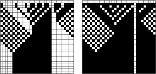
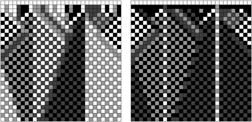
Figure 4 shows the time evolution of $U_j^n$ and ${\tilde{V}}_j^n$ in the case that L = 3. The white, light grey, dark grey and black cells denote zero, one, two and three, respectively. The initial values of ${\tilde{V}}_j^0$ are set as ${\tilde{V}}_8^0=2$, ${\tilde{V}}_{21}^0=1$ and ${\tilde{V}}_j^0=3$ for other j. It can be observed that, at most, two cars are allowed to move forward per unit of time at the point where ${\tilde{V}}_8^n=2$, and at most one car at the point where ${\tilde{V}}_{22}^n=1$. From the above, it can be said that the variable ${\tilde{V}}_j^n$ behaves like a traffic flow controller.

Figure 4. Time evolution of $U_j^n$ (left) and ${\tilde{V}}_j^n$ (right) in the case that L = 3.

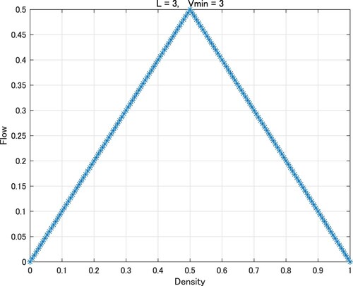
5.2. Fundamental diagrams of the correlated Burgers cellular automata

Consider the fundamental diagrams of the correlated Burgers CA. The density is denoted by $\rho =\frac{1}{NL}\sum _{j=0}^{N-1}{U}_j^n,$and the average flow $Q^n$ at the discrete time n is defined as $Q^n=\frac{1}{NL}\sum _{j=0}^{N-1}min(V_{j+1}^{n-1},U_j^n,L-U_{j+1}^n)=\frac{1}{NL}\sum _{j=0}^{N-1}{X}_{j+1}^n.$Figures 5–10 show the fundamental diagrams with $(L,{\tilde{V}}_{min})=$ (1,1), (2,1), (2,2), (3,1), (3,2), (3,3), where ${\tilde{V}}_{min}:=\underset{j=0,1,\dots ,N-1}{min}{\tilde{V}}_j^0$. In these figures, N = 50, ${\tilde{V}}_j^{-1}=0$ for $j=0,1,\dots ,N-1$ and $U_j^0$ and ${\tilde{V}}_j^0$ for $j=0,1,\dots ,N-1$ are given randomly by integer values between $[0,L]$ and $[{\tilde{V}}_{min},L]$, respectively, where ${\tilde{V}}_j^0$ is set to take ${\tilde{V}}_{min}$ at least one site j. Here, in order to avoid the average flow being zero, ${\tilde{V}}_j^0$ is set as integer greater than or equal to 1. Flows are computed at discrete time n = 100 and are plotted in the figures.

Figure 5. Fundamental diagram of L = 1 and ${\tilde{V}}_{min}=1$.

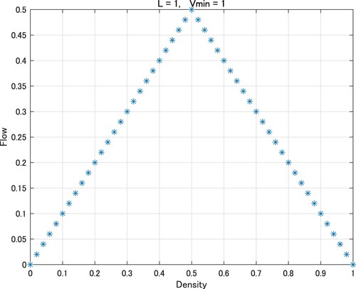
Figure 5 coincides with the fundamental diagram of the original traffic flow model of the elementary CA of rule 184. In Figures 6, 8 and 9, the values of the flow hit the ceiling and adopt a trapezoidal shape. It is evident that the phase transitions at $\rho =0.25$ and 0.75 in Figure 6, $\rho =0.1666\cdots$ and 0.8333··· in Figure 8, and $\rho =0.3333\cdots$ and 0.6666··· in Figure 9.

Figure 6. Fundamental diagram of L = 2 and ${\tilde{V}}_{min}=1$.

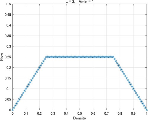
Figure 7. Fundamental diagram of L = 2 and ${\tilde{V}}_{min}=2$.

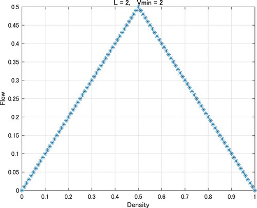
Figure 8. Fundamental diagram of L = 3 and ${\tilde{V}}_{min}=1$.

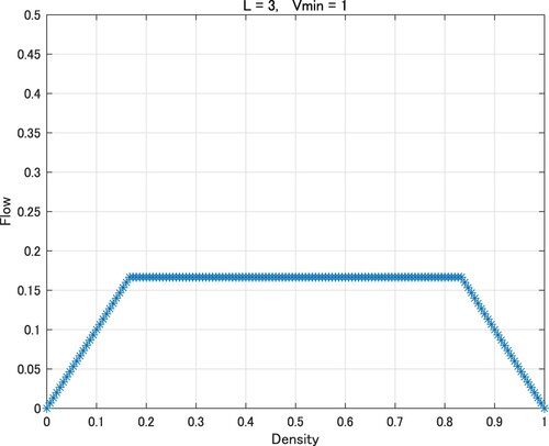
Figure 9. Fundamental diagram of L = 3 and ${\tilde{V}}_{min}=2$.

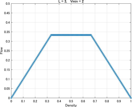
Figure 10. Fundamental diagram of L = 3 and ${\tilde{V}}_{min}=3$.

This result can be explained as follows. Here the average velocity $v^n$ is defined as $v^n=\frac{\sum _{j=0}^{N-1}{X}_j^n}{\sum _{j=0}^{N-1}{U}_j^n}.$The section in which the average velocity of cars is one is called the free flow section and otherwise the jam flow section. In the following, it is assumed that, after sufficient discrete time evolution, the whole N sites will be either (i) only free flow section, (ii) mixed (free and jam) flow section, or (iii) only jam flow section. Let $v_F$ and $v_J$ be the average velocity in free and jam flow section, respectively. Let ${\rho }_F$ and ${\rho }_J$ be the density in free and jam flow section, respectively. Then, the density ρ and the average flow Q of the whole N sites are given by $\begin{array}{rl}\rho & ={\rho }_{J}x+{\rho }_F(1-x),\\ Q& ={\rho }_J{v}_{J}x+{\rho }_F{v}_F(1-x),\end{array}$where x is the ratio of the length of the jam section to N. In the case (i), because there are no jam flow section, $\rho ={\rho }_F$ and $v_F=1$ hold, then the average flow is $Q={\rho }_F{v}_F={\rho }_F=\rho$. In the case (ii), it is assumed that the site $p\in \{0,1,\dots ,N-1\}$ and the discrete time $n_0$ exist such that the whole space is partitioned into the free and jam flow sections at site p after any $n\ge n_0$, that is, sites $j\ge p$ and j<p belong to free and jam flow section, respectively. Then ${\tilde{V}}_p^0={\tilde{V}}_{min}$ holds. If $U_p^n=a$, where $0\le a\le {\tilde{V}}_{min}$, then $U_p^{n+1}={\tilde{V}}_{min}-a$ and $U_{p+1}^{n+1}=a$ hold since the site p−1 belongs to jam flow section and sites p and p + 1 belong to free flow section. At discrete time n + 2, $U_p^{n+2}=a$ and $U_{p+1}^{n+2}={\tilde{V}}_{min}-a$ hold and this behaviour repeat at $n+3,n+4,\dots$. The sequence $\{U_j^n{\}}_{j\ge p}$ yields the alternating sequence of ${\tilde{V}}_{min}-a$ and a in the free flow section for any $n\ge n_0$. Similarly, in the jam flow section, sequence $\{U_j^n{\}}_{j<p}$ yields the alternating sequence of $L-{\tilde{V}}_{min}+a$ and L−a. Therefore, the densities ${\rho }_F$ and ${\rho }_J$ are given by (24) ${\rho }_F=\frac{{\tilde{V}}_{min}}{2L},{\rho }_J=\frac{2L-{\tilde{V}}_{min}}{2L}=1-{\rho }_F.$(24) The average velocities $v_F$, $v_J$ are given by (25) $v_F=\frac{{\tilde{V}}_{min}}{{\tilde{V}}_{min}}=1,v_J=\frac{{\tilde{V}}_{min}}{2L-{\tilde{V}}_{min}}=\frac{{\rho }_F}{1-{\rho }_F}.$(25) From (24(24) ${\rho }_F=\frac{{\tilde{V}}_{min}}{2L},{\rho }_J=\frac{2L-{\tilde{V}}_{min}}{2L}=1-{\rho }_F.$(24) ) and (25(25) $v_F=\frac{{\tilde{V}}_{min}}{{\tilde{V}}_{min}}=1,v_J=\frac{{\tilde{V}}_{min}}{2L-{\tilde{V}}_{min}}=\frac{{\rho }_F}{1-{\rho }_F}.$(25) ), the average flow Q can be written as $Q=(1-{\rho }_F)\frac{{\rho }_F}{1-{\rho }_F}x+{\rho }_F(1-x)={\rho }_F=\frac{{\tilde{V}}_{min}}{2L}.$In the case (iii), because there is no free flow section, $\rho ={\rho }_J$ holds and the average flow Q is given by $Q={\rho }_J{v}_J={\rho }_J\frac{{\tilde{V}}_{min}}{2L-{\tilde{V}}_{min}}=1-{\rho }_J=1-\rho .$Therefore, the fundamental diagram of the correlated Burgers CA is given by $\begin{array}{r}Q=\{\begin{array}{ll}\rho & {\displaystyle \mathrm{if}0\le \rho \le \frac{{\tilde{V}}_{min}}{2L},}\\ {\displaystyle \frac{{\tilde{V}}_{min}}{2L}}& {\displaystyle \mathrm{if}\frac{{\tilde{V}}_{min}}{2L}\le \rho \le 1-\frac{{\tilde{V}}_{min}}{2L},}\\ 1-\rho {\displaystyle }& \mathrm{if}1-{\displaystyle \frac{{\tilde{V}}_{min}}{2L}}\le \rho \le 1.\end{array}\end{array}$Therefore, two first-order phase transition of densities exist whose points are given by $({\rho }^{\ast },Q^{\ast })$ and $(1-{\rho }^{\ast },Q^{\ast })$, where ${\rho }^{\ast }=Q^{\ast }=\frac{{\tilde{V}}_{min}}{2L}.$This result agrees with Figures 5–10.

6. Concluding remarks

This paper focuses on the correlated random walk, which is a type of generalization of the random walks, and it derives the discrete and ultradiscrete diffusion as well as Burgers equations with its corresponding CA. In the traffic flow model derived through the correlated random walk, a car behaves depending on the current and previous states. Such behaviour inherits the non-Markovian of the original correlated random walk. There are many studies on traffic flow models based on Burgers CA and its extensions, as mentioned in Section 1. In the study of the traffic flow model, it is important to analyse the fundamental diagram, and specifically, to identify the phase transition points. The fundamental diagram of the correlated Burgers CA under the assumption of the convergence of dynamics is derived. A direction of future works will be to prove the convergence using the ultradiscrete correlated Burgers equation. Additionally, although the integrability of the conventional diffusion equation and the Burgers equation has already been studied, this study's resulting equations will also be discussed.

Acknowledgments

The authors wish to thank Prof. Daichi Yanagisawa for valuable discussions.

Disclosure statement

No potential conflict of interest was reported by the author(s).

Additional information

Funding

This work was partially supported by the Grant-in-Aid for Early-Career Scientists number 20K14367 and by the Grants-in-Aid for Scientific Research (C) numbers 19K03616 and 19K03624 from the Japan Society for the Promotion of Science (JSPS).

References

- J.D. Cole, On a quasilinear parabolic equation occurring in aerodynamics, Quart. Appl. Math. 9 (1951), pp. 225–236.
- H. Emmerich and B. Kahng, A random cellular automaton related to the noisy Burgers equation, Phys. A 259 (1998), pp. 81–89.
- M. Fukui, K. Nishinari, D. Takahashi, and Y. Ishibashi, Metastable flows in a two-lane traffic model equivalent to extended Burgers cellular automaton, Phys. A 303 (2002), pp. 226–238.
- S. Goldstein, On diffusion by discontinuous movements, and on the telegraph equation, Quart. J. Mech. Appl. Math. 4 (1951), pp. 129–156.
- R. Hirota, Nonlinear partial difference equations reducible to linear equations, J. Phys. Soc. Jpn. 46 (1979), pp. 312–319.
- E. Hopf, The partial differential equation ut+uux=μuxx, Comm. Pure Appl. Math. 3 (1950), pp. 201–230.
- M. Kac, A stochastic model related to the telegrapher's equation, Rocky Mt. J. Math. 4 (1974), pp. 497–509.
- N. Konno, Limit theorems and absorption problems for one-dimensional correlated random walks, Stoch. Models 25 (2009), pp. 28–49.
- C.R. Laing and A. Longtin, Noise-induced stabilization of bumps in systems with long-range spatial coupling, Phys. D 160 (2001), pp. 149–172.
- K. Nishinari and D. Takahashi, Analytical properties of ultradiscrete Burgers equation and rule-184 cellular automaton, J. Phys. A: Math. Gen. 31 (1998), pp. 5439–5450.
- E. Renshaw and R. Henderson, The correlated random walk, J. Appl. Prob. 18 (1981), pp. 403–414.
- T. Tokihiro, D. Takahashi, J. Matsukidaira, and J. Satsuma, From soliton equations to integrable cellular automata through a limiting procedure, Phys. Rev. Lett. 76 (1996), pp. 3247–3250.
- G.H. Weiss, Some applications of persistent random walks and the telegrapher's equation, Phys. A311 (2002), pp. 381–410.