
 ?Mathematical formulae have been encoded as MathML and are displayed in this HTML version using MathJax in order to improve their display. Uncheck the box to turn MathJax off. This feature requires Javascript. Click on a formula to zoom.
Abstract
In this paper, we study iterations of two-dimensional maps, in particular iterations of Lozi maps in the region of the parameter space where it has a strange attractor. Using symbolic dynamics techniques for two-dimensional maps, based on the kneading theory of Milnor and Thurston and also in the symbolic dynamic formalism developed by Sousa Ramos, through the kneading sequence for the Lozi maps, we characterize the region in the parameter space that contains the kneading curves and present a method to define a Markov partition for the Lozi attractors. Consequently, the topological entropy for the Lozi map is computed.
1. Introduction
Consider the following parametrized family of Lozi maps:
(1)
(1) These piecewise linear plane invertible maps were introduced in 1978 by René Lozi [Citation5] as a simplified version of the parametrized family of Hénon maps, without loosing the capacity to show chaotic behaviour. Since then, Lozi maps has been an important tool to understand complex behaviour of iterated maps on the plane.
Since it is an invertible map, it is possible to define its inverse, , given by
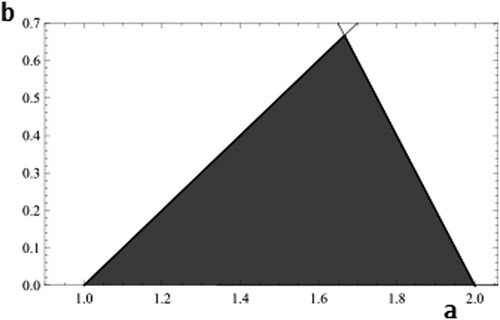
In 1992 [Citation6] Liu et al. showed that for parameters
satisfying
(2)
(2) every map
has indeed a strange attractor. Let
denote the corresponding region of the parameter space; see Figure .
Figure 1. The parameter space region for which has a strange attractor.
Earlier, Michał Misiurewicz [Citation7] introduced a region in
satisfying
(3)
(3) allowing to present the Lozi map attractor,
, from its successive forward iteration,
(4)
(4) Considering the fixed point that lies in the first quadrant
and computing its local stability by evaluating the eigenvalues of the jacobian matrix of the map at the fixed point, in the domain of the parameters for
, the fixed point is a saddle point. Let
and
be the stable and unstable manifolds of
, respectively.
Definition 1.1
The Lozi map fundamental domain is the triangle with vertices
,
, and
, where
(5)
(5) is the intersection point of the unstable manifold of the fixed point
,
, with the horizontal axis.
Next, some definitions of Lozi maps symbolic dynamics are presented, following [Citation4].
Definition 1.2
Given , the itinerary of
is the bi-infinite symbolic sequence
(6)
(6) where the symbols
, for
, are defined as
(7)
(7) where
corresponds to the
component of
.
By the previous definition, is a bi-infinite symbolic sequence of
. It is important to distinguish the itinerary for the past and the itinerary for the future of a point X; let
be an itinerary of
. The symbolic subsequence
is the itinerary for the past of
and the symbolic subsequence
is the itinerary for the future. Thus,
.
2. Critical set
Let be the vertical axis, such that
where
is the nonnegative part of the vertical axis and
is the negative part of the vertical axis.
According to the construction process suggested by Ishii [Citation4] and Baptista et al. [Citation3], some points belonging to play a very important role in the study of Lozi's maps dynamics, especially the point
. The orbit associated with the forward itinerary of the point
is the orbit whose itinerary, for the future, corresponds to the maximum symbolic sequence within the set of all admissible symbolic sequences for the future.
Definition 2.1
Given a Lozi map , its kneading sequence
is the itinerary for the future of
, i.e.
Definition 2.2
Let . Given a Lozi map
, its pruned kneading sequence,
is the initial subsequence of symbols of
such that the first symbol ★ appears at position
, that is,
.
From the inverse map , two maps can be introduced,
and
, as follows:
and
Using these two maps and a pruned kneading sequence,
we will define a certain type of line segments, in
as follows:
Definition 2.3
Let and
for
.
The line segments , with
, in
, are defined by
After the definition of the line segments with
, for n>3, its possible to define the critical set for
when
.
Definition 2.4
Let and
. The critical set
is defined as the set containing the line segments
, with
, the vertical line segment
and the points
and I.
The following proposition presents the slope of each line segment , with
(for n>3).
Proposition 2.5
Let and
. The line segments
, with
, are given by
where
and
Proof.
Let be the pruned kneading sequence of
with dimension
.
Consider the jacobian matrix of at the point
, defined as follows:
and
where
corresponds to the y component of
.
Let be the vector of the line segment
. The vector of a line segment
is given by
Depending on the value of
, the point
will belong to
or
. By the definition of
,
will be a line segment that passes through the point
with vector
and slope
.
Let . As
the slope of the line segment
will be
Therefore, for
, the line segment
that passes through the point
has the vector given by
and slope given by
Proposition 2.6
Let ,
. The intersection of the line segment
with the
is the point
where
Proof.
The line segment (when
) is the vertical line, and its intersection with the
occurs at the point
. The pre-image of
is
. Let
be the slope of the line segments
with
, for
. Therefore, the line segment that passes through the points
and
has slope
and can be given by
. Since this line segment contains the segment
the intersection of the line segment
with the
occurs at the point
.
Continuing this process, the pre-image of the point is the point
. Therefore, the line segment
is contained in a line segment that passes through the point
with slope
and intersects the
at the point
. In general, the pre-image of a point
is the point
and consequently the line segment
with
, for
intersects the
at the point
, where
Considering Propositions 2.5 and 2.6, the next result follows.
Proposition 2.7
Let and
. The line segments
, with
, for
and the vertical line segment
do not intersect.
2.1. Order relation in the set 
From [Citation4], the attractor points with the same fixed itinerary for the past lie in a segment
, called the unstable leaf, completely characterized by the parameter values
and
. Moreover, attractor points with the same fixed itinerary for the future
lie in a segment
, called the stable leaf, also completely characterized by
and
. If a point
has a fixed itinerary
,
is the intersection of the line segments previously defined, denoted by
and
, respectively.
In order to rewrite the order relation established by Ishii [Citation4] for the set , consider the following definition.
Definition 2.8
Let and
be two symbolic subsequences for the future.
if one of the following conditions is satisfied:
the number of
the number of
where the order on the symbols is .
If for all
,
.
From the previous definition it can be establish that, for any point ,
(8)
(8) Considering the set
, where
is the shift-operator, the set
and denoting by
as a permutation in the set
such that
(9)
(9) it follows that
(10)
(10) and where
means that
is on the left side of
, and consequently
(11)
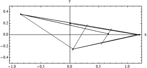
(11) Figure illustrates the critical set, the attractor and the invariant triangle
, considering the pruned kneading sequence
.
Figure 2. The critical set and the Lozi map attractor for the pruned kneading sequence .
2.2. Markov partition on
Using the elements of the critical set where
, it is possible to construct a partition, with
regions, for the set
and therefore to
.
Considering the Definition 2.8 and the order relations given in (Equation9(9)
(9) ), (Equation10
(10)
(10) ) and (Equation11
(11)
(11) ) we define the
regions on the triangle
as follows:
let be a permutation in the set
such that
The
regions on the triangle
are defined as follows:
where
means that
is on the right side of
or
belongs to
and
means that
is on the left side of
.
Considering the previous construction the next result follows:
Theorem 2.9
The set is a topological partition of
.
Let belong to the interior of a set
. Suppose that
where
is single region or a union of two or more regions of the topological partition
. Assume, without loss of generality, that it is a single region. Thus,
Moreover, by Ishii [Citation4], the unstable leaf and the stable leaf of
lie in a segment denoted by
and
, respectively, and X is the intersection point of the segments previously defined. Therefore, and due to the Lozi map linearity, we can state that
and
Thus, by Bowen [Citation2], it follows:
Theorem 2.10
The topological partition provides a Markov partition of
associated to
.
3. Transition matrix and topological entropy
Definition 3.1
Let be a Markov partition of
associated to
. The transition matrix over
is a square matrix
, of order
, such that
Following [Citation8] and [Citation1], the topological entropy of can be calculated using the corresponding transition matrix. This result can be stated as follows:
Proposition 3.2
Let and
. Let
be the transition matrix associated to
. The topological entropy of
is given by
where
is the spectral radius of
.
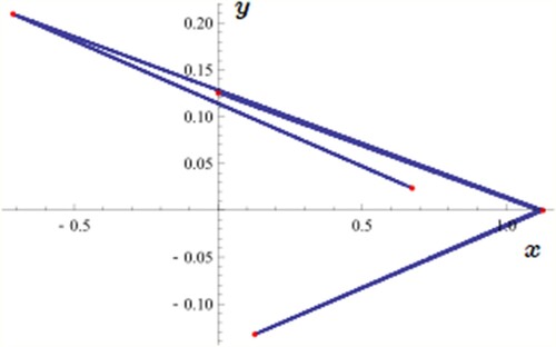
Example 3.3
Let consider and the pruned kneading sequence associated
The itinerary given by the pruned kneading sequence
for
is given in Figure .
Figure 3. Itinerary given by the pruned kneading sequence and Lozi attractor for .
Applying the shift map to the pruned kneading sequence it follows:
By Definition 2.8, the following order relation is valid
and consequently
The partition of
is given through the regions ()
which can be associated to the following transition matrix
given by
The transition matrix
has maximum eigenvalue
and the topological entropy is approximately
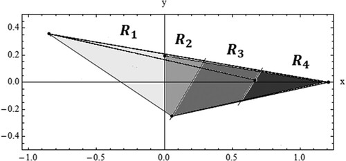
Example 3.4
Consider and the pruned kneading sequence associated
Applying the shift map to
that verifies the following order relationship:
and
The partition of
is given through the regions ()
which can be associated to the following transition matrix
:
The transition matrix
has a maximum eigenvalue
and the topological entropy is approximately
Figure 4. Itinerary of point I, the critical set and the regions , j = 1, 2, 3, 4.
3.1. Isentropics curves for Lozi maps
From [Citation3], a pruned kneading sequence corresponds to an algebraic condition on the parameters and, therefore, to a curve on the parameter plane. For example, a simple computation shows that the kneading curve for the pruned kneading sequence is described by the following condition:
Definition 3.5
Given a pruned kneading sequence of dimension
, its kneading curve
is the parameter space curve corresponding to parameter values such that
.
Following the work [Citation3], and considering Proposition 3.2, the topological entropy of along the curve
is equal to
, where
is the point of the horizontal axis given by the limit, as
, of
and therefore
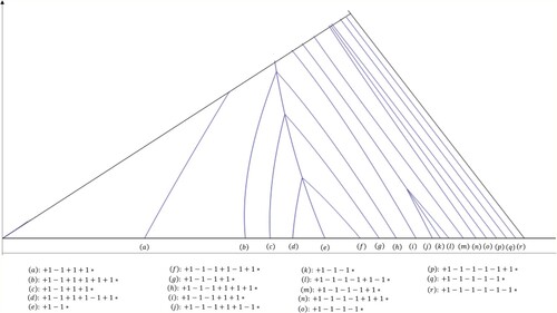
Figure illustrates the kneading curves (isentropic curves) for pruned kneading sequence up to dimension 7.
Figure 5. Itinerary and the partition associated to the pruned kneading sequence when
.
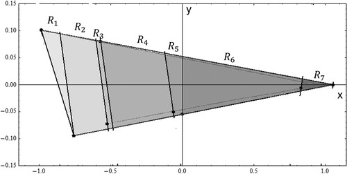
Figure 6. Isentropic curves associated to a pruned kneading sequence.
Acknowledgments
The author expresses his gratitude to Ricardo Severino and Sandra Vinagre for all their support and encouragement in obtaining these results.
Disclosure statement
No potential conflict of interest was reported by the author(s).
Additional information
Funding
References
- V.M. Alekseev and M.V. Yakobson, Symbolic dynamics and hyperbolic dynamic systems, Phys. Rep.75 (1981), pp. 290–325.
- Rufus Bowen, Markov partitions for axiom A diffeomorphisms, Amer. J. Math. 92 (1970), pp. 725–747.
- Diogo Baptista, Ricardo Severino, and Sandra Vinagre, Kneading curves for Lozi maps, Grazer Math. Ber. 354 (2009), pp. 6–14.
- Y. Ishii, Towards a kneading theory for Lozi mappings I: A solution of pruning front conjecture and the first tangency problem, Nonlinearity 10 (1997), pp. 731–747.
- R. Lozi, Un attracteur étrange du type attracteur de Hénon, J. Physique (Paris) 39 (1978), pp. 9–10.
- Z. Liu, H. Xie, Z. Zhu, and Q. Lu, The strange attractor of the Lozi mapping, Int. J. Bifur. Chaos Appl. Sci. Engrg. 2 (1992), pp. 831–839.
- M. Misiurewicz, Strange attractors for the Lozi mappings, in Nonlinear Dynamics, R.G. Helleman, ed., The New York Academy of Sciences, New York, 1980.
- Peter Walters, An introduction to ergodic theory, in Graduate Texts in Mathematics, Vol. 79, Springer-Verlag, New York, 1982.