Modeling the population dynamics and movement of Zebra mussels

Abstract

Zebra mussels have caused significant damage in many lakes and rivers. By using a hybrid population model with discrete-time equations and ordinary differential equations, we represent the zebra mussel's life cycle, growth, and population movement. The dynamics of the larvae (unsettled and settled larvae) are represented during the summer months in a system of two ordinary differential equations, while the juvenile, small adult, and large adult stages are represented by a discrete model with yearly time steps. The goal is to investigate the effects of zebra mussel movement between three different spatial locations and possible control measures. Zebra mussel data and temperature values from three locations in the Hudson River over several years were used to estimate model parameters. We investigate the stability and net reproductive number for our model. We illustrate numerically the hybrid population model for several scenarios of movement and cleaning boats to remove mussels.

Keywords:

• Modeling spread of zebra mussel
• Hudson river
• differential equations
• discrete equations
• boat movement
• natural downstream flow

MATHEMATICS SUBJECT CLASSIFICATIONS:

• 39A60
• 92B05

1. Introduction

The zebra mussel is one of the world's most problematic invasive species, causing large economic damages and major changes to ecosystems [6, 10]. Zebra mussels are small D- or wedge-shaped bivalve (2-shelled) mollusks, which are named after the alternating light and dark brown zigzag pattern on their shells. They live on lake and river bottoms, rocks, aquatic plants, docks, lifts, and boats to which they attach. As many as seven hundred thousand mussels can occupy a surface of a square meter [3, 14]. Once attached, they generally stay in one place but can detach and move to a new location if environmental conditions change [13]. They originated from Eurasia and made their way to North America and the Great Lakes in the ballast water of a ship in the mid 1980s [3, 14]. According to USGS.gov [3], the first two locations of the zebra mussels in the United States were in Lake Erie. Since then, the mussels have spread to over 32 different states by water currents, boats, boat trailers, seaplanes, and other aquatic equipment, causing damages among those who depend on freshwater [3].

Zebra mussels have caused millions of dollars in damages and drastic changes to freshwater ecosystems [6]. Their huge populations attach to hard surfaces, clog intake pipes for water treatment and power generating plants, and encrust boat motors and hulls. Ecologically, they are filter feeders that filter immense amounts of bacteria, plankton (both phytoplankton and zooplankton), and organic debris, which causes large impacts on ecosystems around them [10]. They also smother and cause extinctions of native bivalve mollusks [5, 21].

The zebra mussel life cycle consists of larvae (unsettled and settled), juveniles, and adults. They typically live for about 2-5 years but have been known to have a life span of up to 9 years [3, 5]. As early as one or two years of age, zebra mussels can mature and reproduce. Reproduction typically takes place once the water is warm enough, usually in the spring or summer [5, 11]. An adult female zebra mussel can release up to one million eggs while an adult male zebra mussel can release over two hundred million sperm into the water per year. In these warm waters fertilization then takes place [3, 5, 8, 11].

Larvae emerge from these fertilized eggs within 2 to 5 days. Larvae have two stages, unsettled (free-swimming larvae) and settled (larvae that have settled onto a substrate) [3, 5]. During the unsettled stage, larvae are able to move freely and travel long distances through water currents. Unsettled larvae settle out usually within 35 days after hatching. Once settling begins, larvae attach to underwater substrates, preferably firm or hard surfaces, using durable sticky threads called byssal fibers [3, 5]. The vast majority of larval mortality occurs at or before settlement[3]. After settling, the surviving zebra mussels grow to become juveniles. The maturation of juveniles happens within the first two years. Once matured into adults, zebra mussels continue to grow in size and are then able to reproduce [3, 8, 11].

In the past few decades, a few mathematical models associated with zebra mussels have been developed. Huang and collaborators created a partial differential equation (PDE) hybrid continuous-discrete benthic-drift population model to examine zebra mussels in a river [11]. The larvae were modelled using partial and ordinary differential equations [11]. The PDE model described how larvae dispersed in the river using a reaction-advection-diffusion equation, while the ordinary differential equation (ODE) model described how larvae settled on a substrate after being in the drift. The main focus of the Huang et al. paper was to analyze how the growth and dispersal of a population, the river flow, and the water temperature of a river affect the persistence and spread of zebra mussels. The spatial dynamics of the Huang et al. model was analyzed mathematically by Jin and Zhao; they proved threshold conditions for population persistence in a bounded domain and constructed bounds on the spreading speeds in an unbounded domain [11, 12]. Mari and collaborators created a model that showed the mechanisms of the spread of zebra mussels in the Mississippi-Missouri river system [16]. This model focused on the mutual interactions of the drivers (water bodies and ports connected to the water system) and controls of the zebra mussel invasion. A multilayer model was used to incorporate demographic dynamics such as hydrologic transport and dispersal due to human activities (movement of boats). In the Mari et al. model, mussels could spread by settling on boats and commercial vessels and moving medium and long distances [16].

Additionally, in work by Potapov and Lewis, an optimal control problem was formulated for a model of the adult life stage of an invasive species (zebra mussels) with Allee effect growth in multiple lakes. These lakes were connected by the travel of recreational boats, and the species attached to the boats were moved. The control strategy in this model represented washing the boats to remove mussels as the boats enter or leave the lakes [22].

In our work, we are interested in the effect of cleaning, but we create a more detailed model with hybrid continuous-discrete features consisting of ordinary differential and discrete equations, showcasing the zebra mussel's population growth, survival, and mortality. In this model, the continuous settlement and mortality of larvae on a daily time-step were combined with the yearly breeding season of juveniles and adults. From there, the mathematical model was expanded to include the spread of zebra mussels through the use of boats between successive locations motivated by data from the Hudson River. Our model also differs from other zebra mussel models by connecting data, incorporating the movement of zebra mussels using both natural river flow and boats, and using scenarios to showcase the change in the population distribution.

The main objective of this study was to build a mechanistic hybrid model (continuous-discrete) to investigate the spread of zebra mussels between different spatial locations. Our model was then connected to feasible control actions, particular locations, and data, which produced two other models. The stability and reproductive number of selected models were analyzed. The growth and spread of zebra mussels in different patches under scenarios with changes in boat movement were then illustrated. Control actions were then designed in our model to decrease zebra mussel population levels and the spatial spread.

In the next section, with the use of data, we formulate a baseline hybrid continuous-discrete model to describe the life cycle of zebra mussels and the movement between three patches of zebra mussels. We then follow with parameter estimation in Section 3. These parameters are then used to find the stability and net reproductive number of the model in Section 4. We then follow with scenarios based on zebra mussel spread in Section 5. Lastly, in Section 6 conclusions are given.

2. Hybrid continuous-discrete age-structured patch models

2.1. One patch model

At first, we consider a baseline model to understand the basic dynamics of a zebra mussel population in a single patch, which may represent one part of a series of connected lakes or river locations. In year n, the different stages of the zebra mussels in this baseline model are represented by $v_n$ (density of unsettled larvae), $w_n$ (density of settled larvae), $J(n)$ (density of juveniles), $A_a(n)$ (density of small adults), and $A_b(n)$ (density of large adults). The adult stage of zebra mussels is split into two categories (small and large adults) based on shell size, reproduction level, and needs. Data from the Cary Institute of Ecosystem Studies were used to show the progression through juveniles, small adults, and large adults [4, 23–25]. We consider a hybrid model with discrete time equations for the juvenile and adult life stages and ordinary differential equations for the two stages of the larvae. The system of differential equations is in year n on a small daily grid size (days in the summer) that is continuous in time (using t as days in $(0,\tau )$ where τ is the maximal settlement time of larvae). This system feeds into the age structure discrete-time system with yearly time steps. The coupled system is constructed this way since the larvae life stage is relatively short (at most 35 days) compared to the zebra mussel lifespan (average of 5 years) [11].

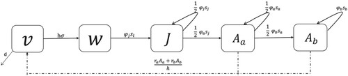
Unsettled larvae either die or settle within 35 days after they emerge. At the end of this period the settled larvae that survive become juveniles. Since zebra mussels stay in the juvenile stage for about two years [8], we assume that, in each year (time step), half of the surviving juveniles remain in that stage and the other half of the surviving juveniles make the transition to small adults. Before the settled larvae move into the juvenile class, existing juveniles will either survive or move to the small adult class. The small adult stage also lasts about two years [8]. Half of them survive an additional year as small adults, while the other half survive to become large adults. Some of the large adults also survive. Small and large adults are able to produce larvae but with possibly different rates. Unsettled larvae stem directly from the number of small and large adults in the preceding year. The zebra mussel's life cycle and dynamics for years $n=0,1,2,\dots$, and time t with $0\le t\le \tau$ (within year n) are given in Figure 1 and modelled as follows (1) $\begin{array}{rl}{v}_n^{\mathrm{\prime }}& =-d{v}_n-\sigma v_n\\ w_n^{\mathrm{\prime }}& =\mathrm{h\sigma }{v}_n\\ J(n+1)& ={\phi }_j(n)[s_l(n)w_n(\tau )+\frac{1}{2}{s}_j(n)J(n)]\\ A_a(n+1)& ={\phi }_a(n)[\frac{1}{2}{s}_j(n)J(n)+\frac{1}{2}{s}_a(n)A_a(n)]\\ A_b(n+1)& ={\phi }_b(n)[\frac{1}{2}{s}_a(n)A_a(n)+s_b(n)A_b(n)]\end{array}$(1) within initial conditions (IC):

Figure 1. One patch model. Baseline model diagram of zebra mussels. Compartments $v_n$, and $w_n$ are on continuous-time $(0,\tau )$ in the summer of year n. Compartments $J(n)$, $A_a(n)$, and $A_b(n)$ are on a discrete-time frame with n representing years. The dash dot line represents the initial condition of unsettled larvae, $v_n$ where n represents the breeding season in years. The initial condition stems directly from reproduction due to the number of small and large adults in the current year.

$v_n(0)=\frac{r_a{A}_a(n)+r_b{A}_b(n)}{h}$, $w_n(0)=0$, $J(0)=J^0$, $A_a(0)=A_a^0$, $A_b(0)=A_b^0$ [8, 11].

Using the solutions, $v_n$ and $w_n$, of (1(1) $\begin{array}{rl}{v}_n^{\mathrm{\prime }}& =-d{v}_n-\sigma v_n\\ w_n^{\mathrm{\prime }}& =\mathrm{h\sigma }{v}_n\\ J(n+1)& ={\phi }_j(n)[s_l(n)w_n(\tau )+\frac{1}{2}{s}_j(n)J(n)]\\ A_a(n+1)& ={\phi }_a(n)[\frac{1}{2}{s}_j(n)J(n)+\frac{1}{2}{s}_a(n)A_a(n)]\\ A_b(n+1)& ={\phi }_b(n)[\frac{1}{2}{s}_a(n)A_a(n)+s_b(n)A_b(n)]\end{array}$(1) ) and initial conditions, $J(n+1)$ can be represented as (2) $\begin{array}{rl}J(n+1)& ={\phi }_j(n)[\frac{s_l(n)\sigma (r_a{A}_a(n)+r_b{A}_b(n))(1-e^{-(d+\sigma )\tau })}{d+\sigma }+\frac{1}{2}{s}_j(n)J(n)]\\ A_a(n+1)& ={\phi }_a(n)[\frac{1}{2}{s}_j(n)J(n)+\frac{1}{2}{s}_a(n)A_a(n)]\\ A_b(n+1)& ={\phi }_b(n)[\frac{1}{2}{s}_a(n)A_a(n)+s_b(n)A_b(n)].\end{array}$(2) Hence, model (2(2) $\begin{array}{rl}J(n+1)& ={\phi }_j(n)[\frac{s_l(n)\sigma (r_a{A}_a(n)+r_b{A}_b(n))(1-e^{-(d+\sigma )\tau })}{d+\sigma }+\frac{1}{2}{s}_j(n)J(n)]\\ A_a(n+1)& ={\phi }_a(n)[\frac{1}{2}{s}_j(n)J(n)+\frac{1}{2}{s}_a(n)A_a(n)]\\ A_b(n+1)& ={\phi }_b(n)[\frac{1}{2}{s}_a(n)A_a(n)+s_b(n)A_b(n)].\end{array}$(2) ) is the final model we will study for the dynamics of zebra mussels in a single patch.

The transitions among the five compartments are illustrated in Figure 1. All variables and parameters of model (2(2) $\begin{array}{rl}J(n+1)& ={\phi }_j(n)[\frac{s_l(n)\sigma (r_a{A}_a(n)+r_b{A}_b(n))(1-e^{-(d+\sigma )\tau })}{d+\sigma }+\frac{1}{2}{s}_j(n)J(n)]\\ A_a(n+1)& ={\phi }_a(n)[\frac{1}{2}{s}_j(n)J(n)+\frac{1}{2}{s}_a(n)A_a(n)]\\ A_b(n+1)& ={\phi }_b(n)[\frac{1}{2}{s}_a(n)A_a(n)+s_b(n)A_b(n)].\end{array}$(2) ) are given in Table 1. However, the units are not given in the table. The differential equations of (1(1) $\begin{array}{rl}{v}_n^{\mathrm{\prime }}& =-d{v}_n-\sigma v_n\\ w_n^{\mathrm{\prime }}& =\mathrm{h\sigma }{v}_n\\ J(n+1)& ={\phi }_j(n)[s_l(n)w_n(\tau )+\frac{1}{2}{s}_j(n)J(n)]\\ A_a(n+1)& ={\phi }_a(n)[\frac{1}{2}{s}_j(n)J(n)+\frac{1}{2}{s}_a(n)A_a(n)]\\ A_b(n+1)& ={\phi }_b(n)[\frac{1}{2}{s}_a(n)A_a(n)+s_b(n)A_b(n)]\end{array}$(1) ) have a daily grid starting with the emergence of larvae from the egg to the day of settlement [3]. Unsettled larvae, $v_n$, are free-swimming larvae that either settle out into $w_n$ with a settling rate of σ or perish with a mortality rate of d. Settled larvae, $w_n$, are unsettled larvae that have successfully attached to a suitable substrate. The transition from unsettled to settled larvae requires a re-scaling of densities because unsettled larvae are microscopic free swimmers whose density is measured per volume of water, while settled larvae are measured based on the surface area they cover. The water depth factor h re-scales the units of unsettled larvae (volume) to the unit of settled larvae (area) [11].

Table 1. Variables and parameters of the baseline model (1(1) $\begin{array}{rl}{v}_n^{\mathrm{\prime }}& =-d{v}_n-\sigma v_n\\ w_n^{\mathrm{\prime }}& =\mathrm{h\sigma }{v}_n\\ J(n+1)& ={\phi }_j(n)[s_l(n)w_n(\tau )+\frac{1}{2}{s}_j(n)J(n)]\\ A_a(n+1)& ={\phi }_a(n)[\frac{1}{2}{s}_j(n)J(n)+\frac{1}{2}{s}_a(n)A_a(n)]\\ A_b(n+1)& ={\phi }_b(n)[\frac{1}{2}{s}_a(n)A_a(n)+s_b(n)A_b(n)]\end{array}$(1) )-(2(2) $\begin{array}{rl}J(n+1)& ={\phi }_j(n)[\frac{s_l(n)\sigma (r_a{A}_a(n)+r_b{A}_b(n))(1-e^{-(d+\sigma )\tau })}{d+\sigma }+\frac{1}{2}{s}_j(n)J(n)]\\ A_a(n+1)& ={\phi }_a(n)[\frac{1}{2}{s}_j(n)J(n)+\frac{1}{2}{s}_a(n)A_a(n)]\\ A_b(n+1)& ={\phi }_b(n)[\frac{1}{2}{s}_a(n)A_a(n)+s_b(n)A_b(n)].\end{array}$(2) ).

Parameters	Interpretation
$v_n(t)$	Density of dispersing (unsettled) larvae on day t, year n
$w_n(t)$	Density of settled larvae on day t, year n
$J(n)$	Density of juveniles in year n
$A_a(n)$	Density of small adults in year n
$A_b(n)$	Density of large adults in year n
$J(0)$	Initial number of juveniles
$A_a(0)$	Initial number of small adults
$A_b(0)$	Initial number of large adults
d	Larval mortality rate
σ	Larval settling rate
h	Water depth
τ	Longest dispersing time before larvae settle
t	Dispersal time of larvae starting in July each year, $0\le t\le \tau$
φ	Density-dependent survival of the population
$s_l$	Larval yearly survival proportion (temperature dependent)
$s_j$	Juvenile yearly survival proportion (temperature dependent)
$s_a$	Small adult yearly survival proportion (temperature dependent)
$s_b$	Large adult yearly survival proportion (temperature dependent)
ys	Monthly survival proportion (temperature dependent)
$r_a$	Reproduction rate of small adults
$r_b$	Reproduction rate of large adults
$S_1$	Survival rate for eggs until the larval life stage
$l_j$	Average shell length of juveniles
$l_a$	Average shell length of small adults
$l_b$	Average shell length of large adults
$s_{l_0}$	Baseline survival of larvae without temperature dependence
$s_{j_0}$	Baseline survival of juveniles without temperature dependence
$s_{a_0}$	Baseline survival of small adults without temperature dependence
$s_{b_0}$	Baseline survival of large adults without temperature dependence
${\beta }_j$	Competition coefficient for juveniles
${\beta }_a$	Competition coefficient for small adults
${\beta }_b$	Competition coefficient for large adults

The dynamics of juveniles, small adults, and large adults of system (2(2) $\begin{array}{rl}J(n+1)& ={\phi }_j(n)[\frac{s_l(n)\sigma (r_a{A}_a(n)+r_b{A}_b(n))(1-e^{-(d+\sigma )\tau })}{d+\sigma }+\frac{1}{2}{s}_j(n)J(n)]\\ A_a(n+1)& ={\phi }_a(n)[\frac{1}{2}{s}_j(n)J(n)+\frac{1}{2}{s}_a(n)A_a(n)]\\ A_b(n+1)& ={\phi }_b(n)[\frac{1}{2}{s}_a(n)A_a(n)+s_b(n)A_b(n)].\end{array}$(2) ) are described by discrete time equations from year n to year n + 1. The juvenile class consists of the settled larvae that survived at the proportion $s_l$ at the time of settlement τ and the juveniles that survived at the proportion $s_j$. Juveniles stay in the juvenile stage for at most 2 years. Thus, one-half of the surviving juveniles stay in the juvenile class, while the other half transition to the small adult class. Just like the juveniles, small adults stay in the small adult stage for at most 2 years. Thus, one-half of the small adults survive at the proportion $s_j$ and stay in the small adult class, while the other half transition to the large adult class. Along with these surviving small adults, the large adult class consists of large adults that survived at a proportion of $s_b$. In discrete models, the order of events is important. Juveniles survive first and one-half make the transition into small adults, then the larvae move in. Small adults survive and then one-half of them make the transition into large adults, and finally, the juveniles move in. Large adults survive and then small adults move in. The last event in the post-larval equations is survival due to density dependence, φ, which is a competition for resources. The density-dependent survival rate of the population φ is given by (3) ${\phi }_x(n)=\frac{1}{1+{\beta }_x[l_{j}J(n)+l_a{A}_a(n)+l_b{A}_b(n)]}$(3) where x = j, a or b, representing juvenile stage, small adult stage, or large adult stage. This function ${\phi }_x$ is similar to a density-dependent term in [11]. In Huang's work, they had a $w(\tau )$ in the denominator, but we do not. This is because, for most of the time in a year, there are no veligers in our river models. Our density-dependent survival rate consists of the competition coefficient ${\beta }_x$ that combines the effect of the average shell length of juveniles, small adults, and large adults, $l_j$, $l_a$, and $l_b$, respectively, and the densities of juveniles, small adults, and large adults.

The initial condition for unsettled larvae represents the density of larvae produced by small and large adults during the breeding season. The dashed line in Figure 1 shows this reproduction. Here the reproduction rates (fecundity) $r_a$ and $r_b$ are the different reproduction rates of larvae based on small and large adult zebra mussels, respectively. For this model, the reproduction rates are as follows (4) $r_p=S_1(e^{2.688+3.40\ln (l_p)})$(4) where p = a or b. These reproduction rates are based on the equations for the annual egg production per adult, $E_p$, and fecundity, $r_p$, the number of larvae reproduced by adults, which were empirically fitted from data by Strayer et al. [24]. They are respectively represented as (5) $\begin{array}{rl}\ln (E_p)& =2.688+3.40\ln (l_p)\\ r_p& =S_1{E}_p\end{array}$(5) where $S_1$ is the survival proportion for eggs until the larvae's life stage. The reproduction rates represent the rate at which small or large adults, respectively, reproduce eggs that survive larval development to become larvae.

We adjusted the reproduction rates of the two adult classes so that their arithmetic mean was 4218 in order to match the reproduction rate in [11]. In addition, since adults stay and reproduce on the bottom surface but larvae disperse in water, to convert the egg size per unit area into the larva size per unit volume, a factor of $\frac{1}{h}$ was used in the initial condition of $v_n$, where h is the water depth. The initial number of settled larvae $w_n(0)$ is assumed to be a density of zero. The data will determine the initial numbers or distributions of juveniles, $J(0)$, small adults, $A_a(0)$, and large adults, $A_b(0)$.

2.2. Study area and data

The area for this study is the Hudson River, see references [24, 25] for details. Three successive sections of the Hudson River were selected as patches. These patches consist of the lower river, middle river, and upper river, and their locations are measured in river kilometres (RKM). RKM is the distance upriver from The Battery at the southern tip of Manhattan. The lower river (RKM 99−151) includes the sites Port Ewen and Poughkeepsie. The middle river (RKM 151−213) includes the sites Coxsackie, Stockport, Stuyvesant, and Tivoli. The upper river (RKM 213−247) includes the sites Albany and Castleton. The total study area consisted of a cumulative area of 140 sq. km. The data reported for the Hudson River was from the years 1994 to 2017.

In the Hudson River data, the density of zebra mussels was organized based on the geographic region of the river, yearly sampling months (June and August), habitat type (rocks and soft sediments), as well as their shell lengths. Typically, 2−3 rocky places plus 3−4 soft-sediment places within each of the 3 geographic strata at each sampling time were sampled. To obtain the data for models (1(1) $\begin{array}{rl}{v}_n^{\mathrm{\prime }}& =-d{v}_n-\sigma v_n\\ w_n^{\mathrm{\prime }}& =\mathrm{h\sigma }{v}_n\\ J(n+1)& ={\phi }_j(n)[s_l(n)w_n(\tau )+\frac{1}{2}{s}_j(n)J(n)]\\ A_a(n+1)& ={\phi }_a(n)[\frac{1}{2}{s}_j(n)J(n)+\frac{1}{2}{s}_a(n)A_a(n)]\\ A_b(n+1)& ={\phi }_b(n)[\frac{1}{2}{s}_a(n)A_a(n)+s_b(n)A_b(n)]\end{array}$(1) )-(2(2) $\begin{array}{rl}J(n+1)& ={\phi }_j(n)[\frac{s_l(n)\sigma (r_a{A}_a(n)+r_b{A}_b(n))(1-e^{-(d+\sigma )\tau })}{d+\sigma }+\frac{1}{2}{s}_j(n)J(n)]\\ A_a(n+1)& ={\phi }_a(n)[\frac{1}{2}{s}_j(n)J(n)+\frac{1}{2}{s}_a(n)A_a(n)]\\ A_b(n+1)& ={\phi }_b(n)[\frac{1}{2}{s}_a(n)A_a(n)+s_b(n)A_b(n)].\end{array}$(2) ), we averaged the data from June and August for both the hard and soft sediments and combined them for each patch location. The bin lengths were then organized to represent the shell sizes of the different life stages of the zebra mussels. From these data, we split the adult class into two separate classes (small adults and large adults). This was initiated to better represent the different needs of these two classes.

According to [3], zebra mussels can grow up to 0.5 mm per day and 1.5−2.0 cm per year. Adult zebra mussels can begin to reproduce when they are 8−9 mm in shell length. This could be within one year in a good growing environment. In regards to shell length, larvae have a shell length of less than 0.1 mm, juveniles have a shell length between 0.1 mm and 7.99 mm, small adults, $A_a$, have a shell length between 8 mm and 17.99 mm, and large adults, $A_b$, have a shell length between 18 mm and 34.99 mm.

For our model, we used the Hudson River data to derive the initial conditions for the juvenile, small adult, and large adult classes for each patch, as seen in Table 2. In addition, we used these data to estimate parameters for simulations, as well as, adapt survival proportions to incorporate the effect of temperature.

Table 2. Initial Conditions of juveniles, small adults, and large adults respectively in patches 1, 2, and 3 at year 0 from data [23–25].

	Upriver	Midriver	Downriver	Units
$J(0)$	5	28	34	$\mathrm{\#}$ of juveniles/m${}^2$
$A_a(0)$	489	6382	2059	$\mathrm{\#}$ of small adults/m${}^2$
$A_b(0)$	503	2559	3092	$\mathrm{\#}$ of large adults/m${}^2$

2.3. Temperature dependent survival proportion

Zebra mussels' growth, reproduction, and mortality depend on water temperature [3, 9, 28]. In the model, we assume that the survival proportions of settled larvae, juveniles, small adults, and large adults depend on temperature. According to [28], the survival of zebra mussels is not usually affected by temperature from $0^{\circ }\mathrm{C}$ up to some upper limiting temperature, which varies with the duration of the high temperature, the physiological condition of the mussel, and the genetic and physiological adaptation of the mussel to high temperatures. At and above the upper limiting temperature, survival falls off sharply.

Temperature-dependent survival of zebra mussels is modelled using a simple ramp-function, where survival is $100\mathrm{\%}$ at temperatures below the upper limiting temperature. Garton et al. suggest that a temperature of ${30}^{\circ }\mathrm{C}$ would be the upper thermal limit for a northern zebra mussel population [9]. That is, survival would be $100\mathrm{\%}$ below ${30}^{\circ }\mathrm{C}$ and $0\mathrm{\%}$ above ${30}^{\circ }\mathrm{C}$. White et al. [28] suggest that a more cautious approach should be taken with the upper thermal limit by using a critical temperature of ${27.5}^{\circ }\mathrm{C}$ [28]. To not have such a drastic effect on survival, we ramp survival from $100\mathrm{\%}$ at ${26}^{\circ }\mathrm{C}$ to $0.1\mathrm{\%}$ at ${29}^{\circ }\mathrm{C}$. The survival proportions are represented as a piecewise function of temperature over three domains. The adjustment factors for survival proportions, $y{s}_k$, depending on the month k and on the average temperature, T, in that month, are given by: (6) $y{s}_k=\{\begin{array}{ll}1& \mathrm{if}T<{26}^{\circ }\mathrm{C}\\ 0.001& \mathrm{if}T>{29}^{\circ }\mathrm{C}\\ -0.3(T-26)+1& \mathrm{Otherwise}\end{array}.$(6) To make our model more realistic, the temperatures for all 12 months in a year were used to find the yearly survival proportion. The adjustment factor for the survival proportion of a month is calculated using the average temperature of that month and then multiplied together with the other monthly survival proportions for that particular year to create the yearly survival proportions as seen in Equation (10(10) $\begin{array}{rl}{v}_{n1}^{\mathrm{\prime }}& =-d{v}_{n1}-\sigma v_{n1}-m_{12}{v}_{n1}\\ v_{n2}^{\mathrm{\prime }}& =-d{v}_{n2}-\sigma v_{n2}+m_{12}{v}_{n1}-m_{23}{v}_{n2}\\ v_{n3}^{\mathrm{\prime }}& =-d{v}_{n3}-\sigma v_{n3}+m_{23}{v}_{n2}\\ w_{n1}^{\mathrm{\prime }}& =\mathrm{h\sigma }{v}_{n1}-z_{12}{w}_{n1}\\ w_{n2}^{\mathrm{\prime }}& =\mathrm{h\sigma }{v}_{n2}+z_{12}{w}_{n1}-z_{23}{w}_{n2}\\ w_{n3}^{\mathrm{\prime }}& =\mathrm{h\sigma }{v}_{n3}+z_{23}{w}_{n2}\end{array}$(10) ): (7) $\begin{array}{rl}{s}_l& =s_{l_0}\cdot \mathrm{ys}\\ s_j& =s_{j_0}\cdot \mathrm{ys}\\ s_a& =s_{a_0}\cdot \mathrm{ys}\\ s_b& =s_{b_0}\cdot \mathrm{ys},\end{array}$(7) where $\mathrm{ys}=\prod _{k=1}^{12}y{s}_k.$Note that each $s_x$ depends on all average monthly temperatures in year n. The constants $s_{l_0}$, $s_{j_0}$, $s_{a_0}$, and $s_{b_0}$, in these equations, represent the baseline survival proportions without water temperature adjustment factors.

Temperature data from the Cary Institute monitoring program were taken from the long-term monitoring station near Kingston, NY [4]. From these data, the temperatures in some months and/or years were missing. The missing temperatures were estimated using previous and post-month temperatures and information from the Weather Underground [27].

2.4. Three patch model

2.4.1. Model with one-way downstream movement

Zebra mussels are able to spread from one location to another through water currents, boats, boat trailers, seaplanes, and other aquatic equipment [3]. This subsection will concentrate on the movement between three patches via natural downstream river flow. This new model represents a closed system without mussels entering from outside or leaving the three patches, and with one-way downstream movement: Patch 1 feeds into patch 2 and patch 2 feeds into patch 3. This model is the same as the one patch model in terms of the life cycle of zebra mussels; see Figure 2. We will expand the one patch model (2(2) $\begin{array}{rl}J(n+1)& ={\phi }_j(n)[\frac{s_l(n)\sigma (r_a{A}_a(n)+r_b{A}_b(n))(1-e^{-(d+\sigma )\tau })}{d+\sigma }+\frac{1}{2}{s}_j(n)J(n)]\\ A_a(n+1)& ={\phi }_a(n)[\frac{1}{2}{s}_j(n)J(n)+\frac{1}{2}{s}_a(n)A_a(n)]\\ A_b(n+1)& ={\phi }_b(n)[\frac{1}{2}{s}_a(n)A_a(n)+s_b(n)A_b(n)].\end{array}$(2) ) to incorporate movements between three geographical locations or patches. We represent the quantities in three patches with subscripts 1, 2, and 3, respectively. The dynamics of zebra mussels with one-way movement in three patches is expressed as follows: (8) $\begin{array}{rl}{v}_{n1}^{\mathrm{\prime }}& =-d{v}_{n1}-\sigma v_{n1}-m_{12}{v}_{n1}\\ v_{n2}^{\mathrm{\prime }}& =-d{v}_{n2}-\sigma v_{n2}+m_{12}{v}_{n1}-m_{23}{v}_{n2}\\ v_{n3}^{\mathrm{\prime }}& =-d{v}_{n3}-\sigma v_{n3}+m_{23}{v}_{n2}\\ w_{n1}^{\mathrm{\prime }}& =\mathrm{h\sigma }{v}_{n1}-z_{12}{w}_{n1}\\ w_{n2}^{\mathrm{\prime }}& =\mathrm{h\sigma }{v}_{n2}+z_{12}{w}_{n1}-z_{23}{w}_{n2}\\ w_{n3}^{\mathrm{\prime }}& =\mathrm{h\sigma }{v}_{n3}+z_{23}{w}_{n2}\\ J_1(n+1)& ={\phi }_{j1}(n)[s_l(n)w_{n1}(\tau )+\frac{1}{2}{s}_j(n)J_1(n)](1-j_{12})\\ J_2(n+1)& ={\phi }_{j2}(n)[s_l(n)w_{n2}(\tau )+\frac{1}{2}{s}_j(n)J_2(n)](1-j_{23})\\ & +j_{12}{\phi }_{j1}(n)[s_l(n)w_{n1}(\tau )+\frac{1}{2}{s}_j(n)J_1(n)]\\ J_3(n+1)& ={\phi }_{j3}(n)[s_l(n)w_{n3}(\tau )+\frac{1}{2}{s}_j(n)J_3(n)]\\ & +j_{23}{\phi }_{j2}(n)[s_l(n)w_{n2}(\tau )+\frac{1}{2}{s}_j(n)J_2(n)]\end{array}$(8) $\begin{array}{rl}{A}_{a1}(n+1)& ={\phi }_{a1}(n)[\frac{1}{2}{s}_j(n)J_1(n)+\frac{1}{2}{s}_a(n)A_{a1}(n)](1-a_{12})\\ A_{a2}(n+1)& ={\phi }_{a2}(n)[\frac{1}{2}{s}_j(n)J_2(n)+\frac{1}{2}{s}_a(n)A_{a2}(n)](1-a_{23})\\ & +a_{12}{\phi }_{a1}(n)[\frac{1}{2}{s}_j(n)J_1(n)+\frac{1}{2}{s}_a(n)A_{a1}(n)]\\ A_{a3}(n+1)& ={\phi }_{a3}(n)[\frac{1}{2}{s}_j(n)J_3(n)+\frac{1}{2}{s}_a(n)A_{a3}(n)]\\ & +a_{23}{\phi }_{a2}(n)[\frac{1}{2}{s}_j(n)J_2(n)+\frac{1}{2}{s}_a(n)A_{a2}(n)]\\ A_{b1}(n+1)& ={\phi }_{b1}(n)[\frac{1}{2}{s}_a(n)A_{a1}(n)+s_b(n)A_{b1}(n)](1-b_{12})\\ A_{b2}(n+1)& ={\phi }_{b2}(n)[\frac{1}{2}{s}_a(n)A_{a2}(n)+s_b(n)A_{b2}(n)](1-b_{23})\\ & +b_{12}{\phi }_{b1}(n)[\frac{1}{2}{s}_a(n)A_{a1}(n)+s_b(n)A_{b1}(n)]\\ A_{b3}(n+1)& ={\phi }_{b3}(n)[\frac{1}{2}{s}_a(n)A_{a3}(n)+s_b(n)A_{b3}(n)]\\ & +b_{23}{\phi }_{b2}(n)[\frac{1}{2}{s}_a(n)A_{a2}(n)+s_b(n)A_{b2}(n)]\end{array}$IC: $v_{\mathrm{ni}}(0)=\frac{r_a{A}_{\mathrm{ai}}(n)+r_b{A}_{\mathrm{bi}}(n)}{h}$, $w_{\mathrm{ni}}(0)=0$, $J_i(0)=J_i^0$, $A_{\mathrm{ai}}(0)=A_{\mathrm{ai}}^0$, $A_{\mathrm{bi}}(0)=A_{\mathrm{bi}}^0$ where $i=1,2,$ or 3.

Figure 2. The three patch model with two-way movement. Without the $j_{21}$, $j_{32}$, $a_{21}$, $a_{32}$, $b_{21}$, and $b_{32}$ arrows, it is the one-way movement model.

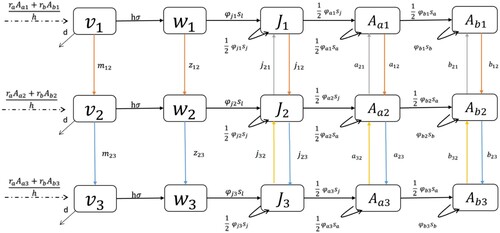
The first three equations show the mortality and settlement of larvae in each patch. Since the equations are in continuous time, all movement happens at the same time. We subtract the movement from one patch and add it to the other patch. We do this for the patch 1 to patch 2 movement and the patch 2 to patch 3 movement. Here, $m_{12}$ represents the rate of unsettled larvae movement from patch 1 to 2, and $m_{23}$ represents the rate of unsettled larvae movement from patch 2 to 3. This same patch movement is used in the settled larvae. According to Kobak, zebra mussels can voluntarily detach from substrates and move or detach depending on certain external factors (such as water movement or substrate material) [13]. The next three equations describe the rate of change of the density of settled larvae in each patch, where $z_{12}$ is the proportion of settled larvae movement from patch 1 to 2 and $z_{23}$ the proportion of settled larvae movement from patch 2 to 3.

After survival, a portion of juvenile, small adult, and large adult zebra mussels in patches 2 move to patch 3 first, then a portion of zebra mussels from patch 1 move to patch 2. On the other hand, juveniles, small adults, and large adults in patch 3 do not move out of their original patch, but the zebra mussels from the other patch are still added in. The last nine equations describe the population growth from year to year in each patch. The movement terms of these discrete equations are different from those in the continuous equations movement. Patch 1 feeds into patch 2 and we subtract the movement from patch 1 and add it to patch 2. We add the movement to patch 2 after we subtract the patch 2 movement to patch 3. Then we add the patch 2 movement to patch 3. In these equations, $j_{12}$ and $j_{23}$ represent juvenile movement from patch 1 to 2 and juvenile movement from patch 2 to patch 3, respectively, while $a_{12}$ and $a_{23}$ represents small adult movement from patch 1 to 2 and adult movement from patch 2 to patch 3, and $b_{12}$ and $b_{23}$ represents large adult movement from patch 1 to 2 and adult movement from patch 2 to patch 3, respectively.

These movement parameters can be seen in Table 3. Unlike in the continuous time equations, we will use $(1-$ proportion moving $)$ to represent the juveniles and/or the adults that stayed in their respective patches and did not move to the next patch, like $(1-j_{12})$. The initial conditions for unsettled larvae in each patch represent the density of larvae reproduced by small and large adults in that patch during the summer breeding season. The initial density of settled larvae $w_{\mathrm{ni}}(0)$ is assumed to be zero for all patches. Then $J_i(0)$, $A_{\mathrm{ai}}(0)$, and $A_{\mathrm{bi}}(0)$ are the initial distributions of juveniles, small adults, and large adults, respectively, in each patch, where $i=1,2,$ or 3. The density-dependent survival proportion function ${\phi }_{\mathrm{xi}}$ in model (8(8) $\begin{array}{rl}{v}_{n1}^{\mathrm{\prime }}& =-d{v}_{n1}-\sigma v_{n1}-m_{12}{v}_{n1}\\ v_{n2}^{\mathrm{\prime }}& =-d{v}_{n2}-\sigma v_{n2}+m_{12}{v}_{n1}-m_{23}{v}_{n2}\\ v_{n3}^{\mathrm{\prime }}& =-d{v}_{n3}-\sigma v_{n3}+m_{23}{v}_{n2}\\ w_{n1}^{\mathrm{\prime }}& =\mathrm{h\sigma }{v}_{n1}-z_{12}{w}_{n1}\\ w_{n2}^{\mathrm{\prime }}& =\mathrm{h\sigma }{v}_{n2}+z_{12}{w}_{n1}-z_{23}{w}_{n2}\\ w_{n3}^{\mathrm{\prime }}& =\mathrm{h\sigma }{v}_{n3}+z_{23}{w}_{n2}\\ J_1(n+1)& ={\phi }_{j1}(n)[s_l(n)w_{n1}(\tau )+\frac{1}{2}{s}_j(n)J_1(n)](1-j_{12})\\ J_2(n+1)& ={\phi }_{j2}(n)[s_l(n)w_{n2}(\tau )+\frac{1}{2}{s}_j(n)J_2(n)](1-j_{23})\\ & +j_{12}{\phi }_{j1}(n)[s_l(n)w_{n1}(\tau )+\frac{1}{2}{s}_j(n)J_1(n)]\\ J_3(n+1)& ={\phi }_{j3}(n)[s_l(n)w_{n3}(\tau )+\frac{1}{2}{s}_j(n)J_3(n)]\\ & +j_{23}{\phi }_{j2}(n)[s_l(n)w_{n2}(\tau )+\frac{1}{2}{s}_j(n)J_2(n)]\end{array}$(8) ) is given by (9) ${\phi }_{\mathrm{xi}}(n)=\frac{1}{1+{\beta }_{\mathrm{xi}}[l_j{J}_i(n)+l_a{A}_{\mathrm{ai}}(n)+l_b{A}_{\mathrm{bi}}(n)]}$(9) where x = j, a or b and $i=1,2,$ or 3.

Table 3. Additional Variables and parameters for the three patch model (8(8) $\begin{array}{rl}{v}_{n1}^{\mathrm{\prime }}& =-d{v}_{n1}-\sigma v_{n1}-m_{12}{v}_{n1}\\ v_{n2}^{\mathrm{\prime }}& =-d{v}_{n2}-\sigma v_{n2}+m_{12}{v}_{n1}-m_{23}{v}_{n2}\\ v_{n3}^{\mathrm{\prime }}& =-d{v}_{n3}-\sigma v_{n3}+m_{23}{v}_{n2}\\ w_{n1}^{\mathrm{\prime }}& =\mathrm{h\sigma }{v}_{n1}-z_{12}{w}_{n1}\\ w_{n2}^{\mathrm{\prime }}& =\mathrm{h\sigma }{v}_{n2}+z_{12}{w}_{n1}-z_{23}{w}_{n2}\\ w_{n3}^{\mathrm{\prime }}& =\mathrm{h\sigma }{v}_{n3}+z_{23}{w}_{n2}\\ J_1(n+1)& ={\phi }_{j1}(n)[s_l(n)w_{n1}(\tau )+\frac{1}{2}{s}_j(n)J_1(n)](1-j_{12})\\ J_2(n+1)& ={\phi }_{j2}(n)[s_l(n)w_{n2}(\tau )+\frac{1}{2}{s}_j(n)J_2(n)](1-j_{23})\\ & +j_{12}{\phi }_{j1}(n)[s_l(n)w_{n1}(\tau )+\frac{1}{2}{s}_j(n)J_1(n)]\\ J_3(n+1)& ={\phi }_{j3}(n)[s_l(n)w_{n3}(\tau )+\frac{1}{2}{s}_j(n)J_3(n)]\\ & +j_{23}{\phi }_{j2}(n)[s_l(n)w_{n2}(\tau )+\frac{1}{2}{s}_j(n)J_2(n)]\end{array}$(8) ) and (10(10) $\begin{array}{rl}{v}_{n1}^{\mathrm{\prime }}& =-d{v}_{n1}-\sigma v_{n1}-m_{12}{v}_{n1}\\ v_{n2}^{\mathrm{\prime }}& =-d{v}_{n2}-\sigma v_{n2}+m_{12}{v}_{n1}-m_{23}{v}_{n2}\\ v_{n3}^{\mathrm{\prime }}& =-d{v}_{n3}-\sigma v_{n3}+m_{23}{v}_{n2}\\ w_{n1}^{\mathrm{\prime }}& =\mathrm{h\sigma }{v}_{n1}-z_{12}{w}_{n1}\\ w_{n2}^{\mathrm{\prime }}& =\mathrm{h\sigma }{v}_{n2}+z_{12}{w}_{n1}-z_{23}{w}_{n2}\\ w_{n3}^{\mathrm{\prime }}& =\mathrm{h\sigma }{v}_{n3}+z_{23}{w}_{n2}\end{array}$(10) ). There is no direct movement between patches 1 and 3.

Variables	Description	Units
$v_{\mathrm{ni}}$	Density of dispersing larvae in drift	Unsettled larvae/ ${\mathrm{m}}^3$
$w_{\mathrm{ni}}$	Density of settled larvae	Settled larvae/${\mathrm{m}}^2$
Parameter	Description	Timescale
Continuous – Time Movement
$m_{12}$	Unsettled larvae movement from patch 1 to 2	Daily
$m_{23}$	Unsettled larvae movement from patch 2 to 3	Daily
$z_{12}$	Settled larvae movement from patch 1 to 2	Daily
$z_{23}$	Settled larvae movement from patch 2 to 3	Daily
Discrete – Time Movement
$j_{12}$	Juvenile movement from patch 1 to 2	Yearly
$j_{23}$	Juvenile movement from patch 2 to 3	Yearly
$a_{12}$	Small adult movement from patch 1 to patch 2	Yearly
$a_{23}$	Small adult movement from patch 2 to patch 3	Yearly
$b_{12}$	Large adult movement from patch 1 to patch 2	Yearly
$b_{23}$	Large adult movement from patch 2 to patch 3	Yearly
$a_{21}$	Small adult movement from patch 2 to patch 1	Yearly
$a_{32}$	Small adult movement from patch 3 to patch 2	Yearly
$b_{21}$	Large adult movement from patch 2 to patch 1	Yearly
$b_{32}$	Large adult movement from patch 3 to patch 2	Yearly

2.4.2. Model with two-way boat movement

In this subsection, we will focus on boat movement, which could increase the spread of the zebra mussels. The two-way boat movement of the three patch model builds off of the one-way movement of the three patch model, as we see in Figure 2. We take the three patch model with one-way movement (8(8) $\begin{array}{rl}{v}_{n1}^{\mathrm{\prime }}& =-d{v}_{n1}-\sigma v_{n1}-m_{12}{v}_{n1}\\ v_{n2}^{\mathrm{\prime }}& =-d{v}_{n2}-\sigma v_{n2}+m_{12}{v}_{n1}-m_{23}{v}_{n2}\\ v_{n3}^{\mathrm{\prime }}& =-d{v}_{n3}-\sigma v_{n3}+m_{23}{v}_{n2}\\ w_{n1}^{\mathrm{\prime }}& =\mathrm{h\sigma }{v}_{n1}-z_{12}{w}_{n1}\\ w_{n2}^{\mathrm{\prime }}& =\mathrm{h\sigma }{v}_{n2}+z_{12}{w}_{n1}-z_{23}{w}_{n2}\\ w_{n3}^{\mathrm{\prime }}& =\mathrm{h\sigma }{v}_{n3}+z_{23}{w}_{n2}\\ J_1(n+1)& ={\phi }_{j1}(n)[s_l(n)w_{n1}(\tau )+\frac{1}{2}{s}_j(n)J_1(n)](1-j_{12})\\ J_2(n+1)& ={\phi }_{j2}(n)[s_l(n)w_{n2}(\tau )+\frac{1}{2}{s}_j(n)J_2(n)](1-j_{23})\\ & +j_{12}{\phi }_{j1}(n)[s_l(n)w_{n1}(\tau )+\frac{1}{2}{s}_j(n)J_1(n)]\\ J_3(n+1)& ={\phi }_{j3}(n)[s_l(n)w_{n3}(\tau )+\frac{1}{2}{s}_j(n)J_3(n)]\\ & +j_{23}{\phi }_{j2}(n)[s_l(n)w_{n2}(\tau )+\frac{1}{2}{s}_j(n)J_2(n)]\end{array}$(8) ) and incorporate two-way boat patch movement. In this model, juveniles, small adults, and large adults move in both directions using boats and natural river flow for downriver movement and only boat movement for upriver movement. Thus, flow driven movement is the same as in the one-way model. Boat movement is then added to this to obtain the new one-way movement for this model. For example, $j_{12}=j_{12c}+j_{12f}$ where the double subscripts, c and f, represent boat movement and flow driven movement, respectively. Boat movement creates a connection between any two patches. This allows the zebra mussels to disperse over long distances throughout a river network [16]. In particular, in our case, it permits the possibility of zebra mussels to move upriver. Unsettled larvae and settled larvae both move using downstream movement. Settled larvae can settle onto boats, but will have survived to the juvenile stage before boat movement can make a significant difference. So, we have four new types of movements. In Table 3, we see that $j_{21}$ and $j_{32}$ represent juvenile movement from patch 2 to patch 1 and from patch 3 to patch 2, respectively, $a_{21}$ and $a_{32}$ represents small adult movement from patch 2 to patch 1 and from patch 3 to patch 2, respectively, and $b_{21}$ and $b_{32}$ represents large adult movement from patch 2 to patch 1 and from patch 3 to patch 2, respectively. Our new system becomes: (10) $\begin{array}{rl}{v}_{n1}^{\mathrm{\prime }}& =-d{v}_{n1}-\sigma v_{n1}-m_{12}{v}_{n1}\\ v_{n2}^{\mathrm{\prime }}& =-d{v}_{n2}-\sigma v_{n2}+m_{12}{v}_{n1}-m_{23}{v}_{n2}\\ v_{n3}^{\mathrm{\prime }}& =-d{v}_{n3}-\sigma v_{n3}+m_{23}{v}_{n2}\\ w_{n1}^{\mathrm{\prime }}& =\mathrm{h\sigma }{v}_{n1}-z_{12}{w}_{n1}\\ w_{n2}^{\mathrm{\prime }}& =\mathrm{h\sigma }{v}_{n2}+z_{12}{w}_{n1}-z_{23}{w}_{n2}\\ w_{n3}^{\mathrm{\prime }}& =\mathrm{h\sigma }{v}_{n3}+z_{23}{w}_{n2}\end{array}$(10) $\begin{array}{rl}{J}_1(n+1)& ={\phi }_{j1}(n)[s_l(n)w_{n1}(\tau )+\frac{1}{2}{s}_j(n)J_1(n)](1-j_{12})\\ & +j_{21}[{\phi }_{j2}(n)[s_l(n)w_{n2}(\tau )+\frac{1}{2}{s}_j(n)J_2(n)](1-j_{23})\\ & +j_{12}{\phi }_{j1}(n)[s_l(n)w_{n1}(\tau )+\frac{1}{2}{s}_j(n)J_1(n)]\\ & +j_{32}[{\phi }_{j3}(n)[s_l(n)w_{n3}(\tau )+\frac{1}{2}{s}_j(n)J_3(n)]\\ & +j_{23}{\phi }_{j2}(n)[s_l(n)w_{n2}(\tau )+\frac{1}{2}{s}_j(n)J_2(n)]]]\\ J_2(n+1)& =[{\phi }_{j2}(n)[s_l(n)w_{n2}(\tau )+\frac{1}{2}{s}_j(n)J_2(n)](1-j_{23})\\ & +j_{12}{\phi }_{j1}(n)[s_l(n)w_{n1}(\tau )+\frac{1}{2}{s}_j(n)J_1(n)]\\ & +j_{32}[{\phi }_{j3}(n)[s_l(n)w_{n3}(\tau )+\frac{1}{2}{s}_j(n)J_3(n)]\\ & +j_{23}{\phi }_{j2}(n)[s_l(n)w_{n2}(\tau )+\frac{1}{2}{s}_j(n)J_2(n)]]](1-j_{21})\\ J_3(n+1)& =[{\phi }_{j3}(n)[s_l(n)w_{n3}(\tau )+\frac{1}{2}{s}_j(n)J_3(n)]\\ & +j_{23}{\phi }_{j2}(n)[s_l(n)w_{n2}(\tau )+\frac{1}{2}{s}_j(n)J_2(n)]](1-j_{32})\end{array}$ $\begin{array}{rl}{A}_{a1}(n+1)& ={\phi }_{a1}(n)[\frac{1}{2}{s}_j(n)J_1(n)+\frac{1}{2}{s}_a(n)A_{a1}(n)](1-a_{12})\\ & +a_{21}[{\phi }_{a2}(n)[\frac{1}{2}{s}_j(n)J_2(n)+\frac{1}{2}{s}_a(n)A_{a2}(n)](1-a_{23})\\ & +a_{12}{\phi }_{a1}(n)[\frac{1}{2}{s}_j(n)J_1(n)+\frac{1}{2}{s}_a(n)A_{a1}(n)]\\ & +a_{32}[{\phi }_{a3}(n)[\frac{1}{2}{s}_j(n)J_3(n)+\frac{1}{2}{s}_a(n)A_{a3}(n)]\\ & +a_{23}{\phi }_{a2}(n)[\frac{1}{2}{s}_j(n)J_2(n)+\frac{1}{2}{s}_a(n)A_{a2}(n)]]]\\ A_{a2}(n+1)& =[{\phi }_{a2}(n)[\frac{1}{2}{s}_j(n)J_2(n)+\frac{1}{2}{s}_a(n)A_{a2}(n)](1-a_{23})\\ & +a_{12}{\phi }_{a1}(n)[\frac{1}{2}{s}_j(n)J_1(n)+\frac{1}{2}{s}_a(n)A_{a1}(n)]\\ & +a_{32}[{\phi }_{a3}(n)[\frac{1}{2}{s}_j(n)J_3(n)+\frac{1}{2}{s}_a(n)A_{a3}(n)]\\ & +a_{23}{\phi }_{a2}(n)[\frac{1}{2}{s}_j(n)J_2(n)+\frac{1}{2}{s}_a(n)A_{a2}(n)]]](1-a_{21})\\ A_{a3}(n+1)& =[{\phi }_{a3}(n)[\frac{1}{2}{s}_j(n)J_3(n)+\frac{1}{2}{s}_a(n)A_{a3}(n)]\\ & +a_{23}{\phi }_{a2}(n)[\frac{1}{2}{s}_j(n)J_2(n)+\frac{1}{2}{s}_a(n)A_{a2}(n)]](1-a_{32})\end{array}$ $\begin{array}{rl}{A}_{b1}(n+1)& ={\phi }_{b1}(n)[\frac{1}{2}{s}_a(n)A_{a1}(n)+s_b(n)A_{b1}(n)](1-b_{12})\\ & +b_{21}[{\phi }_{b2}(n)[\frac{1}{2}{s}_a(n)A_{a2}(n)+s_b(n)A_{b2}(n)](1-b_{23})\\ & +b_{12}{\phi }_{b1}(n)[\frac{1}{2}{s}_a(n)A_{a1}(n)+s_b(n)A_{b1}(n)]\\ & +b_{32}[{\phi }_{b3}(n)[\frac{1}{2}{s}_a(n)A_{a3}(n)+s_b(n)A_{b3}(n)]\\ & +b_{23}{\phi }_{b2}(n)[\frac{1}{2}{s}_a(n)A_{a2}(n)+s_b(n)A_{b2}(n)]]]\\ A_{b2}(n+1)& =[{\phi }_{b2}(n)[\frac{1}{2}{s}_a(n)A_{a2}(n)+s_b(n)A_{b2}(n)](1-b_{23})\\ & +b_{12}{\phi }_{b1}(n)[\frac{1}{2}{s}_a(n)A_{a1}(n)+s_b(n)A_{b1}(n)]\\ & +b_{32}[{\phi }_{b3}(n)[\frac{1}{2}{s}_a(n)A_{a3}(n)+s_b(n)A_{b3}(n)]\\ & +b_{23}{\phi }_{b2}(n)[\frac{1}{2}{s}_a(n)A_{a2}(n)+s_b(n)A_{b2}(n)]]](1-b_{21})\\ A_{b3}(n+1)& =[{\phi }_{b3}(n)[\frac{1}{2}{s}_a(n)A_{a3}(n)+s_b(n)A_{b3}(n)]\\ & +b_{23}{\phi }_{b2}(n)[\frac{1}{2}{s}_a(n)A_{a2}(n)+s_b(n)A_{b2}(n)]](1-b_{32})\end{array}$IC: $v_{\mathrm{ni}}(0)=\frac{r_a{A}_{\mathrm{ai}}(n)+r_b{A}_{\mathrm{bi}}(n)}{h}$, $w_{\mathrm{ni}}(0)=0$, $J_i(0)=J_i^0$, $A_{\mathrm{ai}}(0)=A_{\mathrm{ai}}^0$, $A_{\mathrm{bi}}(0)=A_{\mathrm{bi}}^0$, where $i=1,2,$ or 3.

The order of movement among patches is very important in model (10(10) $\begin{array}{rl}{v}_{n1}^{\mathrm{\prime }}& =-d{v}_{n1}-\sigma v_{n1}-m_{12}{v}_{n1}\\ v_{n2}^{\mathrm{\prime }}& =-d{v}_{n2}-\sigma v_{n2}+m_{12}{v}_{n1}-m_{23}{v}_{n2}\\ v_{n3}^{\mathrm{\prime }}& =-d{v}_{n3}-\sigma v_{n3}+m_{23}{v}_{n2}\\ w_{n1}^{\mathrm{\prime }}& =\mathrm{h\sigma }{v}_{n1}-z_{12}{w}_{n1}\\ w_{n2}^{\mathrm{\prime }}& =\mathrm{h\sigma }{v}_{n2}+z_{12}{w}_{n1}-z_{23}{w}_{n2}\\ w_{n3}^{\mathrm{\prime }}& =\mathrm{h\sigma }{v}_{n3}+z_{23}{w}_{n2}\end{array}$(10) ) just like the other models. Note that the proportion of zebra mussels from patch 1 moves in patch 2 after the proportion of patch 2 zebra mussels moves to patch 3. Following the initial downriver movement, the mussels move upriver. Starting at patch 3, a proportion of the combined zebra mussels move to patch 2. After the move to patch 2, a proportion of the combined zebra mussels in patch 2 move to patch 1, as seen in Figure 2.

3. Parameter estimation

Parameter estimation was used to obtain unknown parameters for the hybrid models. Parameters were estimated separately for the one patch model (1(1) $\begin{array}{rl}{v}_n^{\mathrm{\prime }}& =-d{v}_n-\sigma v_n\\ w_n^{\mathrm{\prime }}& =\mathrm{h\sigma }{v}_n\\ J(n+1)& ={\phi }_j(n)[s_l(n)w_n(\tau )+\frac{1}{2}{s}_j(n)J(n)]\\ A_a(n+1)& ={\phi }_a(n)[\frac{1}{2}{s}_j(n)J(n)+\frac{1}{2}{s}_a(n)A_a(n)]\\ A_b(n+1)& ={\phi }_b(n)[\frac{1}{2}{s}_a(n)A_a(n)+s_b(n)A_b(n)]\end{array}$(1) )-(2(2) $\begin{array}{rl}J(n+1)& ={\phi }_j(n)[\frac{s_l(n)\sigma (r_a{A}_a(n)+r_b{A}_b(n))(1-e^{-(d+\sigma )\tau })}{d+\sigma }+\frac{1}{2}{s}_j(n)J(n)]\\ A_a(n+1)& ={\phi }_a(n)[\frac{1}{2}{s}_j(n)J(n)+\frac{1}{2}{s}_a(n)A_a(n)]\\ A_b(n+1)& ={\phi }_b(n)[\frac{1}{2}{s}_a(n)A_a(n)+s_b(n)A_b(n)].\end{array}$(2) ), for the three patch model with one-way movement (8(8) $\begin{array}{rl}{v}_{n1}^{\mathrm{\prime }}& =-d{v}_{n1}-\sigma v_{n1}-m_{12}{v}_{n1}\\ v_{n2}^{\mathrm{\prime }}& =-d{v}_{n2}-\sigma v_{n2}+m_{12}{v}_{n1}-m_{23}{v}_{n2}\\ v_{n3}^{\mathrm{\prime }}& =-d{v}_{n3}-\sigma v_{n3}+m_{23}{v}_{n2}\\ w_{n1}^{\mathrm{\prime }}& =\mathrm{h\sigma }{v}_{n1}-z_{12}{w}_{n1}\\ w_{n2}^{\mathrm{\prime }}& =\mathrm{h\sigma }{v}_{n2}+z_{12}{w}_{n1}-z_{23}{w}_{n2}\\ w_{n3}^{\mathrm{\prime }}& =\mathrm{h\sigma }{v}_{n3}+z_{23}{w}_{n2}\\ J_1(n+1)& ={\phi }_{j1}(n)[s_l(n)w_{n1}(\tau )+\frac{1}{2}{s}_j(n)J_1(n)](1-j_{12})\\ J_2(n+1)& ={\phi }_{j2}(n)[s_l(n)w_{n2}(\tau )+\frac{1}{2}{s}_j(n)J_2(n)](1-j_{23})\\ & +j_{12}{\phi }_{j1}(n)[s_l(n)w_{n1}(\tau )+\frac{1}{2}{s}_j(n)J_1(n)]\\ J_3(n+1)& ={\phi }_{j3}(n)[s_l(n)w_{n3}(\tau )+\frac{1}{2}{s}_j(n)J_3(n)]\\ & +j_{23}{\phi }_{j2}(n)[s_l(n)w_{n2}(\tau )+\frac{1}{2}{s}_j(n)J_2(n)]\end{array}$(8) ), and for the three patch model with two-way movement (10(10) $\begin{array}{rl}{v}_{n1}^{\mathrm{\prime }}& =-d{v}_{n1}-\sigma v_{n1}-m_{12}{v}_{n1}\\ v_{n2}^{\mathrm{\prime }}& =-d{v}_{n2}-\sigma v_{n2}+m_{12}{v}_{n1}-m_{23}{v}_{n2}\\ v_{n3}^{\mathrm{\prime }}& =-d{v}_{n3}-\sigma v_{n3}+m_{23}{v}_{n2}\\ w_{n1}^{\mathrm{\prime }}& =\mathrm{h\sigma }{v}_{n1}-z_{12}{w}_{n1}\\ w_{n2}^{\mathrm{\prime }}& =\mathrm{h\sigma }{v}_{n2}+z_{12}{w}_{n1}-z_{23}{w}_{n2}\\ w_{n3}^{\mathrm{\prime }}& =\mathrm{h\sigma }{v}_{n3}+z_{23}{w}_{n2}\end{array}$(10) ), due to the different types of movements (no movement, one-way downstream movement, and two-way boat movement). Table 4 shows the parameter values that will be estimated for each model as well as the parameters that were obtained from the literature or the parameters calculated from data. MATLAB optimization tools, MultiStart with fmincon, were used for parameter estimation to directly estimate the best parameter solutions to the problem [19].

Table 4. Parameters for models (1(1) $\begin{array}{rl}{v}_n^{\mathrm{\prime }}& =-d{v}_n-\sigma v_n\\ w_n^{\mathrm{\prime }}& =\mathrm{h\sigma }{v}_n\\ J(n+1)& ={\phi }_j(n)[s_l(n)w_n(\tau )+\frac{1}{2}{s}_j(n)J(n)]\\ A_a(n+1)& ={\phi }_a(n)[\frac{1}{2}{s}_j(n)J(n)+\frac{1}{2}{s}_a(n)A_a(n)]\\ A_b(n+1)& ={\phi }_b(n)[\frac{1}{2}{s}_a(n)A_a(n)+s_b(n)A_b(n)]\end{array}$(1) ), (8(8) $\begin{array}{rl}{v}_{n1}^{\mathrm{\prime }}& =-d{v}_{n1}-\sigma v_{n1}-m_{12}{v}_{n1}\\ v_{n2}^{\mathrm{\prime }}& =-d{v}_{n2}-\sigma v_{n2}+m_{12}{v}_{n1}-m_{23}{v}_{n2}\\ v_{n3}^{\mathrm{\prime }}& =-d{v}_{n3}-\sigma v_{n3}+m_{23}{v}_{n2}\\ w_{n1}^{\mathrm{\prime }}& =\mathrm{h\sigma }{v}_{n1}-z_{12}{w}_{n1}\\ w_{n2}^{\mathrm{\prime }}& =\mathrm{h\sigma }{v}_{n2}+z_{12}{w}_{n1}-z_{23}{w}_{n2}\\ w_{n3}^{\mathrm{\prime }}& =\mathrm{h\sigma }{v}_{n3}+z_{23}{w}_{n2}\\ J_1(n+1)& ={\phi }_{j1}(n)[s_l(n)w_{n1}(\tau )+\frac{1}{2}{s}_j(n)J_1(n)](1-j_{12})\\ J_2(n+1)& ={\phi }_{j2}(n)[s_l(n)w_{n2}(\tau )+\frac{1}{2}{s}_j(n)J_2(n)](1-j_{23})\\ & +j_{12}{\phi }_{j1}(n)[s_l(n)w_{n1}(\tau )+\frac{1}{2}{s}_j(n)J_1(n)]\\ J_3(n+1)& ={\phi }_{j3}(n)[s_l(n)w_{n3}(\tau )+\frac{1}{2}{s}_j(n)J_3(n)]\\ & +j_{23}{\phi }_{j2}(n)[s_l(n)w_{n2}(\tau )+\frac{1}{2}{s}_j(n)J_2(n)]\end{array}$(8) ), and (10(10) $\begin{array}{rl}{v}_{n1}^{\mathrm{\prime }}& =-d{v}_{n1}-\sigma v_{n1}-m_{12}{v}_{n1}\\ v_{n2}^{\mathrm{\prime }}& =-d{v}_{n2}-\sigma v_{n2}+m_{12}{v}_{n1}-m_{23}{v}_{n2}\\ v_{n3}^{\mathrm{\prime }}& =-d{v}_{n3}-\sigma v_{n3}+m_{23}{v}_{n2}\\ w_{n1}^{\mathrm{\prime }}& =\mathrm{h\sigma }{v}_{n1}-z_{12}{w}_{n1}\\ w_{n2}^{\mathrm{\prime }}& =\mathrm{h\sigma }{v}_{n2}+z_{12}{w}_{n1}-z_{23}{w}_{n2}\\ w_{n3}^{\mathrm{\prime }}& =\mathrm{h\sigma }{v}_{n3}+z_{23}{w}_{n2}\end{array}$(10) ).

Parameters from Literature
Parameters	Interpretation	Values
h	Water depth	8 [24]
d	Larval mortality rate	0.086 [11]
σ	Larval settling rate	0.00144 [11]
τ	Longest dispersing time before larvae settle	35 [11]
Parameters Calculated or Obtained from Data
Parameters	Interpretation	Values
$r_a$	Reproduction rate of small adults	947
$r_b$	Reproduction rate of large adults	3,271
$S_1$	Survival rate for eggs until the larval life stage	0.01201[24]
$E_a$	Annual egg production of small adults	78,864[24]
$E_b$	Annual egg production of small adults	272,465[24]
$l_j$	Average shell length of juveniles	6 [23–25]
$l_a$	Average shell length of small adults	12.5 [23–25]
$l_b$	Average shell length of large adults	18 [23–25]
Estimated Parameters
Parameters	Interpretation	Values
$s_{l_0}$	Baseline survival of larvae without temperature dependence	–
$s_{j_0}$	Baseline survival of juveniles without temperature dependence	–
$s_{a_0}$	Baseline survival of small adults without temperature dependence	–
$s_{b_0}$	Baseline survival of large adults without temperature dependence	–
${\beta }_j$	Competition coefficient for juveniles	–
${\beta }_a$	Competition coefficient for small adults	–
${\beta }_b$	Competition coefficient for large adults	–
$m_{12}=m_{23}$	Unsettled larval downriver movement	–
$z_{12}=z_{23}$	Settled larval downriver movement	–
$j_{12}=j_{23}$	Juvenile downriver movement	–
$a_{12}=a_{23}$	Small adult downriver movement	–
$b_{12}=b_{23}$	Large adult downriver movement	–
$j_{21}=j_{32}$	Juvenile upriver movement	–
$a_{23}=a_{32}$	Small adult upriver movement	–
$b_{21}=b_{32}$	Large adult upriver movement	–

The MultiStart algorithm and the local solver, fmincon, are from the Global Optimization Toolbox in MATLAB. The MultiStart algorithm starts at fmincon from multiple start points to find multiple initial values that lead to the same local minimum and in turn the global minimum. The local solver, fmincon, is a nonlinear programming solver that is used to find the minimum of a problem or constrained nonlinear multivariable function. MultiStart has three basic steps: generate start points, run start points, and create GlobalOptimSolutions vectors. MultiStart stops when a vector of GlobalOptimSolution objects is created using local solutions sorted by objective function value, which produces the best result to estimate parameters [17, 18, 20].

In other words, first, MultiStart checks the input of the problem for validity by using fmincon once on problem inputs. Secondly, MultiStart generates k−1 start points for the number of k starting points requested by the user. MultiStart chooses starting points based on a uniform distribution (i.e. equal probability for each point to be chosen) within the parameter bounds provided. Then, MultiStart runs fmincon with the user-chosen starting points. Here, fmincon checks to see if the user-prescribed maximum time has passed at each of its iterations. If the maximum time has passed then fmincon exits the iteration without reporting a solution. MultiStart stops when there are no more starting points or if the maximum time has passed. Once MultiStart stops, a vector of GlobalOptimSolution objects is created using local solutions that were sorted by objective function value from lowest to best. Thus, the best result from the iterations is used to estimate parameters within the bounds provided [17, 18, 20].

This objective function or error consists of multiple terms for the simulated number of juveniles, young adults, and mature adults, respectively. For each life stage and each patch, the distance between the simulated zebra mussel densities and the corresponding densities from data is calculated using the Euclidean norm of the difference between the vector elements. These norms are then divided by the norm of the zebra mussel densities from the data. From there, the calculations for each life stage and patch are combined and weighted: (11) $\begin{array}{r}\text{Objective Function}=0.4\sum _{i=1}^3\frac{\Vert \mathrm{DiffJ}(\mathrm{i})\Vert }{\Vert \mathrm{DataJ}(\mathrm{i})\Vert }+0.3\sum _{i=1}^3\frac{\Vert \mathrm{DiffAa}(\mathrm{i})\Vert }{\Vert \mathrm{DataAa}(\mathrm{i})\Vert }+0.3\sum _{i=1}^3\frac{\Vert \mathrm{DiffAb}(\mathrm{i})\Vert }{\Vert \mathrm{DataAb}(\mathrm{i})\Vert }\end{array}$(11) where the difference between the simulated value and the data is represented using DiffJ, DiffAa, or DiffAb, such as subtracting the vectors, $\mathrm{DiffJ}=\mathrm{SimulatedJ}-\mathrm{DataJ}$. The life stage respective data is represented as DataJ, DataAa, or DataAb.

For the models in this section, we wanted to show how population levels fluctuated over the years. This was to make the model realistic compared to the data fluctuation. MultiStart, in this case, was used to estimate parameters. Due to this, the bounds for the parameters in all three models started off very wide. While estimating parameters for the three patch models, each type of movement term was the same for all the patches for simplicity. The movement for larvae (unsettled and settled), juveniles, and small and large adults, respectively, are the same from patch 1 to patch 2 and from patch 2 to patch 3. Furthermore, movement from patch 3 to patch 2 and from patch 2 to patch 1 are the same for their respective zebra mussel life stage. These movements are considered two-way or upstream movements, which can only be done using boats.

The number of starting points ranged from 5 to 50. The starting bound ranges were decided based on the different behaviour of the life stages in the data. From these observations, parameters were estimated that depicted realistic models. The one patch model uses the estimated parameters in Table 5 to simulate the fluctuations in the densities of juveniles and small and large adults from 1994 to 2017 if no dispersal were incorporated, as seen in Figure 3. The three patch model with one-way and two-way movements used the respective parameters in Table 5 to show the fluctuations of the total zebra mussels in all three patches when dispersal was assumed, as seen in Figures 4 and 5. Since the three patch models with one way and two way movement were formed using the baseline one patch model, we build off of the parameter estimation of the one patch model to estimate the parameters needed for movement in the three patch models. As we can see, the corresponding movement rates for Figures 4 and 5 are identical, but the number of zebra mussels from Table 5 differ when comparing the one-way and two-way movement. Without the outliers in the beginning years, it is easier to see the fluctuation of the zebra mussels. By using parameter estimation, we were able to depict realistic zebra mussel population growth and/or zebra mussel spread within one patch and between three patches.

Figure 3. Simulation results for the total number of juveniles, small adults, and large adults in the one patch model using estimated parameters. The y-axis unit is the number of zebra mussels per square metre.

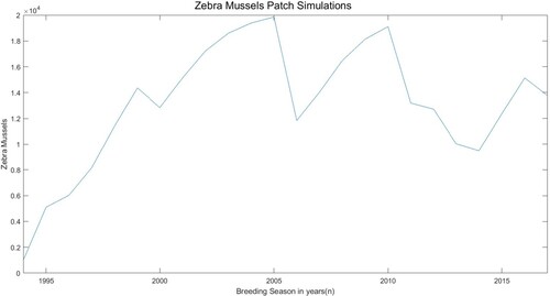
Figure 4. Simulated total population (sum of juveniles, small adults, and large adults) for the three patch model with one-way downstream movement using estimated parameters in Table 5. The y-axis unit is the number of zebra mussels per square metre.

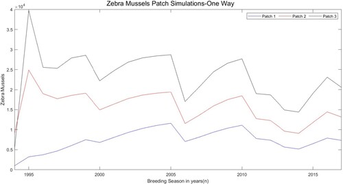
Figure 5. Simulated total population (sum of juveniles, small adults, and large adults) for the three patch model with two-way boat movement using estimated parameters in Table 5. The y-axis unit is the number of zebra mussels per square metre.

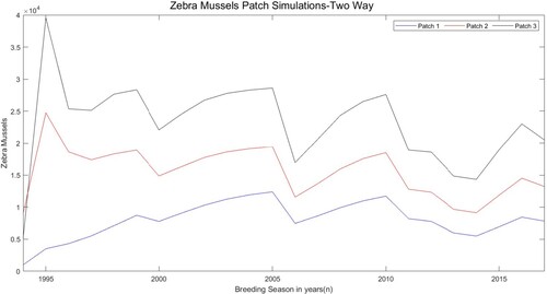
Table 5. Parameter estimates for models. The parameters for the one patch model are also used in the three patch one-way model and the three patch two-way model.

One Patch		Three Patch		Three Patch
(1(1) $\begin{array}{rl}{v}_n^{\mathrm{\prime }}& =-d{v}_n-\sigma v_n\\ w_n^{\mathrm{\prime }}& =\mathrm{h\sigma }{v}_n\\ J(n+1)& ={\phi }_j(n)[s_l(n)w_n(\tau )+\frac{1}{2}{s}_j(n)J(n)]\\ A_a(n+1)& ={\phi }_a(n)[\frac{1}{2}{s}_j(n)J(n)+\frac{1}{2}{s}_a(n)A_a(n)]\\ A_b(n+1)& ={\phi }_b(n)[\frac{1}{2}{s}_a(n)A_a(n)+s_b(n)A_b(n)]\end{array}$(1) )-(2(2) $\begin{array}{rl}J(n+1)& ={\phi }_j(n)[\frac{s_l(n)\sigma (r_a{A}_a(n)+r_b{A}_b(n))(1-e^{-(d+\sigma )\tau })}{d+\sigma }+\frac{1}{2}{s}_j(n)J(n)]\\ A_a(n+1)& ={\phi }_a(n)[\frac{1}{2}{s}_j(n)J(n)+\frac{1}{2}{s}_a(n)A_a(n)]\\ A_b(n+1)& ={\phi }_b(n)[\frac{1}{2}{s}_a(n)A_a(n)+s_b(n)A_b(n)].\end{array}$(2) )		One-Way (8(8) $\begin{array}{rl}{v}_{n1}^{\mathrm{\prime }}& =-d{v}_{n1}-\sigma v_{n1}-m_{12}{v}_{n1}\\ v_{n2}^{\mathrm{\prime }}& =-d{v}_{n2}-\sigma v_{n2}+m_{12}{v}_{n1}-m_{23}{v}_{n2}\\ v_{n3}^{\mathrm{\prime }}& =-d{v}_{n3}-\sigma v_{n3}+m_{23}{v}_{n2}\\ w_{n1}^{\mathrm{\prime }}& =\mathrm{h\sigma }{v}_{n1}-z_{12}{w}_{n1}\\ w_{n2}^{\mathrm{\prime }}& =\mathrm{h\sigma }{v}_{n2}+z_{12}{w}_{n1}-z_{23}{w}_{n2}\\ w_{n3}^{\mathrm{\prime }}& =\mathrm{h\sigma }{v}_{n3}+z_{23}{w}_{n2}\\ J_1(n+1)& ={\phi }_{j1}(n)[s_l(n)w_{n1}(\tau )+\frac{1}{2}{s}_j(n)J_1(n)](1-j_{12})\\ J_2(n+1)& ={\phi }_{j2}(n)[s_l(n)w_{n2}(\tau )+\frac{1}{2}{s}_j(n)J_2(n)](1-j_{23})\\ & +j_{12}{\phi }_{j1}(n)[s_l(n)w_{n1}(\tau )+\frac{1}{2}{s}_j(n)J_1(n)]\\ J_3(n+1)& ={\phi }_{j3}(n)[s_l(n)w_{n3}(\tau )+\frac{1}{2}{s}_j(n)J_3(n)]\\ & +j_{23}{\phi }_{j2}(n)[s_l(n)w_{n2}(\tau )+\frac{1}{2}{s}_j(n)J_2(n)]\end{array}$(8) )		Two-Way (10(10) $\begin{array}{rl}{v}_{n1}^{\mathrm{\prime }}& =-d{v}_{n1}-\sigma v_{n1}-m_{12}{v}_{n1}\\ v_{n2}^{\mathrm{\prime }}& =-d{v}_{n2}-\sigma v_{n2}+m_{12}{v}_{n1}-m_{23}{v}_{n2}\\ v_{n3}^{\mathrm{\prime }}& =-d{v}_{n3}-\sigma v_{n3}+m_{23}{v}_{n2}\\ w_{n1}^{\mathrm{\prime }}& =\mathrm{h\sigma }{v}_{n1}-z_{12}{w}_{n1}\\ w_{n2}^{\mathrm{\prime }}& =\mathrm{h\sigma }{v}_{n2}+z_{12}{w}_{n1}-z_{23}{w}_{n2}\\ w_{n3}^{\mathrm{\prime }}& =\mathrm{h\sigma }{v}_{n3}+z_{23}{w}_{n2}\end{array}$(10) )
Parameter	Estimate	Parameter	Estimate	Parameter	Estimate
$s_{l_0}$	0.60	$m_{12}=m_{23}$	0.06	$j_{12}=j_{23}$	0.017
$s_{j_0}$	0.73	$z_{12}=z_{23}$	0.003	$a_{12}=a_{23}$	0.028
$s_{a_0}$	0.85	$j_{12}=j_{23}$	0.007	$b_{12}=b_{23}$	0.039
$s_{b_0}$	0.80	$a_{12}=a_{23}$	0.008	$j_{21}=j_{32}$	0.01
${\beta }_j$	0.000003	$b_{12}=b_{23}$	0.009	$a_{21}=a_{32}$	0.02
${\beta }_a$	0.0000057			$b_{21}=b_{32}$	0.03
${\beta }_b$	0.0000075

4. Model analysis

4.1. Net reproductive number for one patch model

The net reproductive number, denoted by ${\mathrm{\Re }}_0$, is the average number of offspring produced per individual in their lifetime. If ${\mathrm{\Re }}_0>1$, then the population is expected to persist in the long run, while if ${\mathrm{\Re }}_0<1$, then the population may go toward extinction. This quantity is obtained by using he linearization of the nonlinear model at the trivial solution, which essentially is a matrix model with the coefficient matrix called a projection matrix, P. According to [11], the projection matrix is the sum of the transition matrix, T, and fertility matrix, F, i.e., P = F + T. Assume that $s_j$, $s_a$, and $s_b$ are constant. The linearization of (2(2) $\begin{array}{rl}J(n+1)& ={\phi }_j(n)[\frac{s_l(n)\sigma (r_a{A}_a(n)+r_b{A}_b(n))(1-e^{-(d+\sigma )\tau })}{d+\sigma }+\frac{1}{2}{s}_j(n)J(n)]\\ A_a(n+1)& ={\phi }_a(n)[\frac{1}{2}{s}_j(n)J(n)+\frac{1}{2}{s}_a(n)A_a(n)]\\ A_b(n+1)& ={\phi }_b(n)[\frac{1}{2}{s}_a(n)A_a(n)+s_b(n)A_b(n)].\end{array}$(2) ) at the equilibrium (0,0,0) can be written as (12) $\left[\begin{array}{c}J(n+1)\\ A_a(n+1)\\ A_b(n+1)\end{array}\right]=\left[\begin{array}{ccc}{\displaystyle \frac{1}{2}}{s}_j& {\displaystyle \frac{s_l{r}_a\sigma (1-e^{-(d+\sigma )\tau })}{d+\sigma }}& {\displaystyle \frac{s_l{r}_b\sigma (1-e^{-(d+\sigma )\tau })}{d+\sigma }}\\ {\displaystyle \frac{1}{2}}{s}_j& {\displaystyle \frac{1}{2}}{s}_a& 0\\ 0& {\displaystyle \frac{1}{2}}{s}_a& s_b\end{array}\right]\left[\begin{array}{c}J(n)\\ A_a(n)\\ A_b(n)\end{array}\right].$(12) The projection matrix in (12(12) $\left[\begin{array}{c}J(n+1)\\ A_a(n+1)\\ A_b(n+1)\end{array}\right]=\left[\begin{array}{ccc}{\displaystyle \frac{1}{2}}{s}_j& {\displaystyle \frac{s_l{r}_a\sigma (1-e^{-(d+\sigma )\tau })}{d+\sigma }}& {\displaystyle \frac{s_l{r}_b\sigma (1-e^{-(d+\sigma )\tau })}{d+\sigma }}\\ {\displaystyle \frac{1}{2}}{s}_j& {\displaystyle \frac{1}{2}}{s}_a& 0\\ 0& {\displaystyle \frac{1}{2}}{s}_a& s_b\end{array}\right]\left[\begin{array}{c}J(n)\\ A_a(n)\\ A_b(n)\end{array}\right].$(12) ) is given as (13) $T=\left[\begin{array}{ccc}{\displaystyle \frac{1}{2}}{s}_j& 0& 0\\ {\displaystyle \frac{1}{2}}{s}_j& {\displaystyle \frac{1}{2}}{s}_a& 0\\ 0& {\displaystyle \frac{1}{2}}{s}_a& s_b\end{array}\right]\mathrm{and}F=\left[\begin{array}{ccc}0& {\displaystyle \frac{s_l{r}_a\sigma (1-e^{-(d+\sigma )\tau })}{d+\sigma }}& {\displaystyle \frac{s_l{r}_b\sigma (1-e^{-(d+\sigma )\tau })}{d+\sigma }}\\ 0& 0& 0\\ 0& 0& 0\end{array}\right].$(13) The net reproductive number for (2(2) $\begin{array}{rl}J(n+1)& ={\phi }_j(n)[\frac{s_l(n)\sigma (r_a{A}_a(n)+r_b{A}_b(n))(1-e^{-(d+\sigma )\tau })}{d+\sigma }+\frac{1}{2}{s}_j(n)J(n)]\\ A_a(n+1)& ={\phi }_a(n)[\frac{1}{2}{s}_j(n)J(n)+\frac{1}{2}{s}_a(n)A_a(n)]\\ A_b(n+1)& ={\phi }_b(n)[\frac{1}{2}{s}_a(n)A_a(n)+s_b(n)A_b(n)].\end{array}$(2) ) is defined as ${\mathrm{\Re }}_0=\rho [F(I-T{)}^{-1}]$ where $\rho (\cdot )$ is the spectral radius of $F(I-T{)}^{-1}$ [2]. Note that (14) $\begin{array}{rl}& F(I-T{)}^{-1}\\ & =[\begin{array}{c}{\displaystyle \frac{\frac{1}{2}{s}_j{s}_l\alpha (1-e^{-(d+\alpha )\tau })(r_a(1-s_b)+\frac{1}{2}{r}_b{s}_a)}{(d+\alpha )(1-\frac{1}{2}{s}_j)(1-\frac{1}{2}{s}_a)(1-s_b)}}\\ 0\\ 0\end{array}\\ & \begin{array}{c}{\displaystyle \frac{s_l\alpha (1-\frac{1}{2}{s}_j)(1-e^{-(d+\alpha )\tau })(r_a(1-s_b)+\frac{1}{2}{r}_b{s}_a)}{(d+\alpha )(1-\frac{1}{2}{s}_j)(1-\frac{1}{2}{s}_a)(1-s_b)}}\\ 0\\ 0\end{array}\\ & \begin{array}{c}{\displaystyle \frac{s_l{r}_b\alpha (1-\frac{1}{2}{s}_j)(1-\frac{1}{2}{s}_a)(1-e^{-(d+\alpha )\tau })}{(d+\alpha )(1-\frac{1}{2}{s}_j)(1-\frac{1}{2}{s}_a)(1-s_b)}}\\ 0\\ 0\end{array}].\end{array}$(14) By using the methods in [7], we can obtain the net reproductive number of the one patch model (2(2) $\begin{array}{rl}J(n+1)& ={\phi }_j(n)[\frac{s_l(n)\sigma (r_a{A}_a(n)+r_b{A}_b(n))(1-e^{-(d+\sigma )\tau })}{d+\sigma }+\frac{1}{2}{s}_j(n)J(n)]\\ A_a(n+1)& ={\phi }_a(n)[\frac{1}{2}{s}_j(n)J(n)+\frac{1}{2}{s}_a(n)A_a(n)]\\ A_b(n+1)& ={\phi }_b(n)[\frac{1}{2}{s}_a(n)A_a(n)+s_b(n)A_b(n)].\end{array}$(2) ): (15) ${\mathrm{\Re }}_0=\frac{\frac{1}{2}{s}_j{s}_l\alpha (1-e^{-(d+\alpha )\tau })(r_a(1-s_b)+\frac{1}{2}{r}_b{s}_a)}{(d+\alpha )(1-\frac{1}{2}{s}_j)(1-\frac{1}{2}{s}_a)(1-s_b)}.$(15) Similarly as in [12], we can use the theory in [26] to establish that the sign of $R_0-1$ is the same as the sign of $\lambda -1$ where λ is the dominant eigenvalue of the projection matrix P. Thus, if ${\mathrm{\Re }}_0>1$, then the equilibrium $(0,0,0)$ of (2(2) $\begin{array}{rl}J(n+1)& ={\phi }_j(n)[\frac{s_l(n)\sigma (r_a{A}_a(n)+r_b{A}_b(n))(1-e^{-(d+\sigma )\tau })}{d+\sigma }+\frac{1}{2}{s}_j(n)J(n)]\\ A_a(n+1)& ={\phi }_a(n)[\frac{1}{2}{s}_j(n)J(n)+\frac{1}{2}{s}_a(n)A_a(n)]\\ A_b(n+1)& ={\phi }_b(n)[\frac{1}{2}{s}_a(n)A_a(n)+s_b(n)A_b(n)].\end{array}$(2) ) is unstable and hence the zebra mussel population will be persistent, and if ${\mathrm{\Re }}_0<1$, then $(0,0,0)$ is locally stable for (2(2) $\begin{array}{rl}J(n+1)& ={\phi }_j(n)[\frac{s_l(n)\sigma (r_a{A}_a(n)+r_b{A}_b(n))(1-e^{-(d+\sigma )\tau })}{d+\sigma }+\frac{1}{2}{s}_j(n)J(n)]\\ A_a(n+1)& ={\phi }_a(n)[\frac{1}{2}{s}_j(n)J(n)+\frac{1}{2}{s}_a(n)A_a(n)]\\ A_b(n+1)& ={\phi }_b(n)[\frac{1}{2}{s}_a(n)A_a(n)+s_b(n)A_b(n)].\end{array}$(2) ) and hence the zebra mussel population will become extinct if the initial population density is small enough.

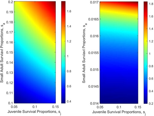
By changing the survival proportions of our model, ${\mathrm{\Re }}_0$ can change from ${\mathrm{\Re }}_0>1$ to ${\mathrm{\Re }}_0<1$. We calculated ${\mathrm{\Re }}_0$ in two cases: $(1)$ where $s_j$ and $s_a$ vary but $s_l$ and $s_b$ are fixed and $(2)$ where $s_j$ and $s_b$ vary but $s_l$ and $s_a$ are fixed; see Figure 6. As survival proportions increase so too does the reproductive number. Thus, if one could control survival proportions, eradication may be possible. Since the survival proportions depend on temperature, these results also indicate that rivers with certain temperature conditions are more favourable to zebra mussels.

Figure 6. The influence of survival proportions on ${\mathrm{\Re }}_0$ for the one patch model. (a) ${\mathrm{\Re }}_0(s_j,s_a)$: Assuming that $s_l$ and $s_b$ are fixed, where $s_l=0.555$ and $s_b=0.74$. (b) ${\mathrm{\Re }}_0(s_j,s_b)$: Assuming that $s_l$ and $s_a$ are fixed, where $s_l=0.555$ and $s_a=0.7863$.

4.2. Analysis of three patch model (10)

We now look at the stability of the three patch model with two-way movement. Again, we assume that the survival terms do not depend on time n through the temperature. Recall that $0<d,\sigma <1,0<d+\sigma <1,0<s_j,s_l,s_a<1,r_a>1,r_b>1,\tau >1.$Suppose that $m_{12}=m_{23}$, $z_{12}=z_{23}$. We start by finding $v_{n1}$ using the initial conditions to get (16) $v_{n1}(t)=v_{n1}(0)e^{-q_{1}t},$(16) where $q_1=d+\sigma +m_{12}$. We then substitute $v_{n1}(t)$ into $v_{n2}^{\mathrm{\prime }}(t)$ and solve for $v_{n2}(t)$ using the initial condition to get (17) $v_{n2}(t)=(v_{n2}(0)+m_{12}{v}_{n1}(0)t)e^{-q_{2}t},$(17) where $q_2=d+\sigma +m_{23}$. We then substitute $v_{n2}(t)$ into $v_{n3}^{\mathrm{\prime }}(t)$ and solve for $v_{n3}(t)$ using the initial condition to get (18) $\begin{array}{rl}{v}_{n3}(t)& =e^{-(d+\sigma )t}{v}_{n3}(0)+(-e^{-q_{2}t}+e^{-(d+\sigma )t})v_{n2}(0)\\ & +(e^{-(d+\sigma )t}-e^{-q_{2}t}(m_{23}t+1))v_{n1}(0).\end{array}$(18) We then substitute $v_{n1}(t)$ into $w_{n1}^{\mathrm{\prime }}(t)$ and solve for $w_{n1}(t)$: (19) $w_{n1}(t)=\frac{\mathrm{h\sigma }{v}_{n1}(0)}{z_{12}-q_1}(e^{-q_{1}t}-e^{-z_{12}t}).$(19) We then substitute $v_{n2}(t)$ and $w_{n1}(t)$ into $w_{n2}^{\mathrm{\prime }}(t)$ and solve for $w_{n2}$: (20) $\begin{array}{rl}{w}_{n2}(t)& =\frac{\mathrm{h\sigma }{v}_{n2}(0)}{z_{23}-q_2}(e^{-q_{2}t}-e^{-z_{23}t})+\frac{\mathrm{h\sigma }{m}_{12}{v}_{n1}(0)}{(z_{23}-q_2{)}^2}(t(z_{23}-q_2)e^{-q_{2}t}-e^{-q_{2}t}\\ & +e^{-z_{23}t})+\frac{\mathrm{h\sigma }{v}_{n1}(0)}{(z_{12}-q_1)(z_{23}-q_1)}(e^{-q_{1}t}-e^{-z_{23}t}-(z_{23}-q_1)t{e}^{-z_{23}t}).\end{array}$(20) We then substitute $v_{n3}(t)$ and $w_{n2}(t)$ into $w_{n3}^{\mathrm{\prime }}(t)$ and solve for $w_{n3}(t)$: (21) $\begin{array}{rl}{w}_{n3}(t)& =\mathrm{h\sigma }(\frac{-(e^{-(d+\sigma )t}-1)v_{n3}(0)}{d+\sigma }+(\frac{e^{-q_{2}t}-1}{q_2}-\frac{e^{-(d+\sigma )t}-1}{d+\sigma })v_{n2}(0)\\ & +(-\frac{e^{-(d+\sigma )t}-1}{d+\sigma }+\frac{m_{23}}{(q_2{)}^2}(t{q}_2{e}^{-q_{2}t}+(e^{-q_{2}t}-1))+\frac{e^{-q_{2}t}-1}{q_2})v_{n1}(0))\\ & +z_{23}(\frac{\mathrm{h\sigma }{m}_{12}{v}_{n1}(0)}{(z_{23}-q_2{)}^2}(\frac{-(z_{23}-q_2)}{(q_2{)}^2}(t{q}_2{e}^{-q_{2}t}+(e^{-q_{2}t}-1))+\frac{e^{-q_{2}t}-1}{q_2}\\ & -\frac{e^{-z_{23}t}-1}{z_{23}})+\frac{\mathrm{h\sigma }{v}_{n1}(0)}{(z_{12}-q_1)(z_{23}-q_1)}(-\frac{(e^{-q_{1}t}-1)}{q_1}+\frac{(e^{-z_{23}t}-1)}{z_{23}}\\ & +\frac{(z_{23}-q_1)}{(z_{23}{)}^2}(t{z}_{23}{e}^{-z_{23}t}+(e^{-z_{23}t}-1)))).\end{array}$(21) After solving for the settled larvae for each patch, we input them into their respective Juvenile patch class. On the right hand sides of the new $J(n+1)$, $A_a(n+1)$, and $A_b(n+1)$ equations we can obtain the projection matrix for the three patch model with two way movement. Using the same methods as in 4.1, we numerically calculate the net reproductive number ${\mathrm{\Re }}_0$ with varying survival proportions, see Figure 7. Here, ${\mathrm{\Re }}_0$ was calculated with varying $s_j$ and $s_a$ and fixed $s_l$ and $s_b$, and with varying $s_j$ and $s_b$ and fixed $s_l$ and $s_a$. 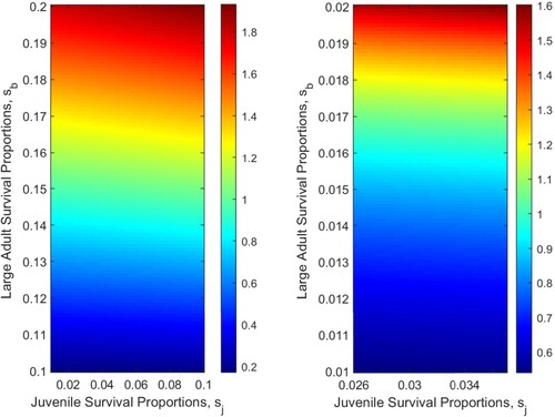The change of ${\mathrm{\Re }}_0$ from below to above 1 can be seen in this figure. Again, we see that as survival proportions increase, the net reproductive number will increase.

Figure 7. The influence of survival proportions on ${\mathrm{\Re }}_0$ for the three patch model with two-way movement. (a) ${\mathrm{\Re }}_0(s_j,s_a)$: Assuming that $s_l$ and $s_b$ are fixed, where $s_l=0.555$ and $s_b=0.74$. (b) ${\mathrm{\Re }}_0(s_j,s_b)$: Assuming that $s_l$ and $s_a$ are fixed, where $s_l=0.555$ and $s_a=0.7863$.

5. Scenarios: Zebra mussel spread

Zebra mussels have been able to spread to over 32 different states by water currents, boats, boat trailers, seaplanes, and other aquatic equipment [3]. This section will focus on three scenarios where the focal point is the movement of zebra mussels via natural river flow and boats. In these scenarios, we assume that larvae are only moving via the natural flow of the river, while the movements of juveniles and adults are occurring by boats and natural river flow in the three patch model with two-way movement (10(10) $\begin{array}{rl}{v}_{n1}^{\mathrm{\prime }}& =-d{v}_{n1}-\sigma v_{n1}-m_{12}{v}_{n1}\\ v_{n2}^{\mathrm{\prime }}& =-d{v}_{n2}-\sigma v_{n2}+m_{12}{v}_{n1}-m_{23}{v}_{n2}\\ v_{n3}^{\mathrm{\prime }}& =-d{v}_{n3}-\sigma v_{n3}+m_{23}{v}_{n2}\\ w_{n1}^{\mathrm{\prime }}& =\mathrm{h\sigma }{v}_{n1}-z_{12}{w}_{n1}\\ w_{n2}^{\mathrm{\prime }}& =\mathrm{h\sigma }{v}_{n2}+z_{12}{w}_{n1}-z_{23}{w}_{n2}\\ w_{n3}^{\mathrm{\prime }}& =\mathrm{h\sigma }{v}_{n3}+z_{23}{w}_{n2}\end{array}$(10) ). To efficiently see how much zebra mussels can spread, we will focus on movement starting in patch 1 and movement starting in patch 3.

In the first scenario, we will assume that no zebra mussels were in the midriver and downriver locations, using the initial number of patch 1 upriver zebra mussels as in Table 2. In the second scenario, we assume that no zebra mussels were in the upriver and midriver locations, using the initial number of patch 3 downriver zebra mussels as in Table 2. In the third scenario, the survival proportions and movement rates are increased to observe the spread when there is either more movement or more growth. In these scenarios, we will also look at the effect of introducing a cleaning factor that either removes $50\mathrm{\%}$ or $99\mathrm{\%}$ of zebra mussels moving on boats.

5.1. Scenario 1: spread starting upriver

We begin with zebra mussels only being in the upriver patch. Starting in patch 1 there are 5 juveniles, 489 small adults, and 503 large adults, per square metre in the year 1994. The other two patches start with zero zebra mussels. By the year 2017, as seen in Table 6, the number of zebra mussels increased drastically. In particular, patch 3 had almost triple the amount of zebra mussels as patch 1. This shows us that boat movement and flow driven movement helps spread zebra mussels to zebra mussel-free locations. To help slow down the spread of zebra mussels, actions can be taken. Boat cleaning, inspections, and interception can help in this aspect. Thus, if we add a cleaning factor, 1−cf, to our models when a boat moves into a new patch, we can lessen the spread. To see an example of this, we implement the cleaning factor for the two-way movement below: (22) $\begin{array}{rl}{J}_1(n+1)& ={\phi }_{j1}(n)[s_l(n)w_{n1}(\tau )+\frac{1}{2}{s}_j(n)J_1(n)](1-j_{12})\\ & +(1-\mathrm{cf})j_{21}[{\phi }_{j2}(n)[s_l(n)w_{n2}(\tau )+\frac{1}{2}{s}_j(n)J_2(n)](1-j_{23})\\ & +((1-\mathrm{cf})j_{{12}_c}+j_{{12}_f}){\phi }_{j1}(n)[s_l(n)w_{n1}(\tau )+\frac{1}{2}{s}_j(n)J_1(n)]\\ & +(1-\mathrm{cf})j_{32}[{\phi }_{j3}(n)[s_l(n)w_{n3}(\tau )+\frac{1}{2}{s}_j(n)J_3(n)]\\ & +((1-\mathrm{cf})j_{{23}_c}+j_{{23}_f}){\phi }_{j2}(n)[s_l(n)w_{n2}(\tau )+\frac{1}{2}{s}_j(n)J_2(n)]]]\\ J_2(n+1)& =[{\phi }_{j2}(n)[s_l(n)w_{n2}(\tau )+\frac{1}{2}{s}_j(n)J_2(n)](1-j_{23})\\ & +((1-\mathrm{cf})j_{{12}_c}+j_{{12}_f}){\phi }_{j1}(n)[s_l(n)w_{n1}(\tau )+\frac{1}{2}{s}_j(n)J_1(n)]\\ & +(1-\mathrm{cf})j_{32}[{\phi }_{j3}(n)[s_l(n)w_{n3}(\tau )+\frac{1}{2}{s}_j(n)J_3(n)]\\ & +((1-\mathrm{cf})j_{{23}_c}+j_{{23}_f}){\phi }_{j2}(n)[s_l(n)w_{n2}(\tau )+\frac{1}{2}{s}_j(n)J_2(n)]]](1-j_{21})\\ J_3(n+1)& =[{\phi }_{j3}(n)[s_l(n)w_{n3}(\tau )+\frac{1}{2}{s}_j(n)J_3(n)]\\ & +((1-\mathrm{cf})j_{{23}_c}+j_{{23}_f}){\phi }_{j2}(n)[s_l(n)w_{n2}(\tau )+\frac{1}{2}{s}_j(n)J_2(n)]](1-j_{32})\end{array}$(22) $\begin{array}{rl}{A}_{a1}(n+1)& ={\phi }_{a1}(n)[\frac{1}{2}{s}_j(n)J_1(n)+\frac{1}{2}{s}_a(n)A_{a1}(n)](1-a_{12})\\ & +(1-\mathrm{cf})a_{21}[{\phi }_{a2}(n)[\frac{1}{2}{s}_j(n)J_2(n)+\frac{1}{2}{s}_a(n)A_{a2}(n)](1-a_{23})\\ & +((1-\mathrm{cf})a_{{12}_c}+a_{{12}_f}){\phi }_{a1}(n)[\frac{1}{2}{s}_j(n)J_1(n)+\frac{1}{2}{s}_a(n)A_{a1}(n)]\\ & +(1-\mathrm{cf})a_{32}[{\phi }_{a3}(n)[\frac{1}{2}{s}_j(n)J_3(n)+\frac{1}{2}{s}_a(n)A_{a3}(n)]\\ & +((1-\mathrm{cf})a_{{23}_c}+a_{{23}_f}){\phi }_{a2}(n)[\frac{1}{2}{s}_j(n)J_2(n)+\frac{1}{2}{s}_a(n)A_{a2}(n)]]]\\ A_{a2}(n+1)& =[{\phi }_{a2}(n)[\frac{1}{2}{s}_j(n)J_2(n)+\frac{1}{2}{s}_a(n)A_{a2}(n)](1-a_{23})\\ & +((1-\mathrm{cf})a_{{12}_c}+a_{{12}_f}){\phi }_{a1}(n)[\frac{1}{2}{s}_j(n)J_1(n)+\frac{1}{2}{s}_a(n)A_{a1}(n)](1-\mathrm{cf})a_{32}\\ & \times [{\phi }_{a3}(n)[\frac{1}{2}{s}_j(n)J_3(n)+\frac{1}{2}{s}_a(n)A_{a3}(n)]\\ & +((1-\mathrm{cf})a_{{23}_c}+a_{{23}_f}){\phi }_{a2}(n)[\frac{1}{2}{s}_j(n)J_2(n)+\frac{1}{2}{s}_a(n)A_{a2}(n)]]](1-a_{21})\\ A_{a3}(n+1)& =[{\phi }_{a3}(n)[\frac{1}{2}{s}_j(n)J_3(n)+\frac{1}{2}{s}_a(n)A_{a3}(n)]\\ & +((1-\mathrm{cf})a_{{23}_c}+a_{{23}_f}){\phi }_{a2}(n)[\frac{1}{2}{s}_j(n)J_2(n)+\frac{1}{2}{s}_a(n)A_{a2}(n)]](1-a_{32})\end{array}$ $\begin{array}{rl}{A}_{b1}(n+1)& ={\phi }_{b1}(n)[\frac{1}{2}{s}_a(n)A_{a1}(n)+s_b(n)A_{b1}(n)](1-b_{12})\\ & +(1-\mathrm{cf})b_{21}[{\phi }_{b2}(n)[\frac{1}{2}{s}_a(n)A_{a2}(n)+s_b(n)A_{b2}(n)](1-b_{23})\\ & +((1-\mathrm{cf})b_{{12}_c}+b_{{12}_f}){\phi }_{b1}(n)[\frac{1}{2}{s}_a(n)A_{a1}(n)+s_b(n)A_{b1}(n)]\\ & +(1-\mathrm{cf})b_{32}[{\phi }_{b3}(n)[\frac{1}{2}{s}_a(n)A_{a3}(n)+s_b(n)A_{b3}(n)]\\ & +((1-\mathrm{cf})b_{{23}_c}+b_{{23}_f}){\phi }_{b2}(n)[\frac{1}{2}{s}_a(n)A_{a2}(n)+s_b(n)A_{b2}(n)]]]\\ A_{b2}(n+1)& =[{\phi }_{b2}(n)[\frac{1}{2}{s}_a(n)A_{a2}(n)+s_b(n)A_{b2}(n)](1-b_{23})\\ & +((1-\mathrm{cf})b_{{12}_c}+b_{{12}_f}){\phi }_{b1}(n)[\frac{1}{2}{s}_a(n)A_{a1}(n)+s_b(n)A_{b1}(n)]\\ & +(1-\mathrm{cf})b_{32}[{\phi }_{b3}(n)[\frac{1}{2}{s}_a(n)A_{a3}(n)+s_b(n)A_{b3}(n)]\\ & +((1-\mathrm{cf})b_{{23}_c}+b_{{23}_f}){\phi }_{b2}(n)[\frac{1}{2}{s}_a(n)A_{a2}(n)+s_b(n)A_{b2}(n)]]](1-b_{21})\\ A_{b3}(n+1)& =[{\phi }_{b3}(n)[\frac{1}{2}{s}_a(n)A_{a3}(n)+s_b(n)A_{b3}(n)]\\ & +((1-\mathrm{cf})b_{{23}_c}+b_{{23}_f}){\phi }_{b2}(n)[\frac{1}{2}{s}_a(n)A_{a2}(n)+s_b(n)A_{b2}(n)]](1-b_{32})\end{array}$where the double subscripts, c and f, represent boat movement and flow driven movement, respectively. With the addition of the cleaning factor 0.5, zebra mussel numbers did decrease a little, as we can see in Table 6. The cleaning factor decreased the number of zebra mussels by about $4.8\mathrm{\%}$. Due to zebra mussels continued growth over the years, the cleaning factor effect is harder to see. If we increased the cleaning factor to $99\mathrm{\%}$. The number of zebra mussels in the two-way movement model decreases more, as seen in Table 6. This new cleaning factor decreased the number of zebra mussels by $9.2\mathrm{\%}$. Figure 8 shows the population size in the patches through time when there was a cleaning factor of either $0\mathrm{\%}$, $50\mathrm{\%}$, or $99\mathrm{\%}$.

Figure 8. Population size of zebra mussels from 1994 to 2017 with a cleaning factor of either $0\mathrm{\%}$, $50\mathrm{\%}$, or $99\mathrm{\%}$. Scenario starting in patch 1 (upriver) where the initial number of juveniles, small adults, and large adults in year 1994 are 5, 489, and 503, respectively.

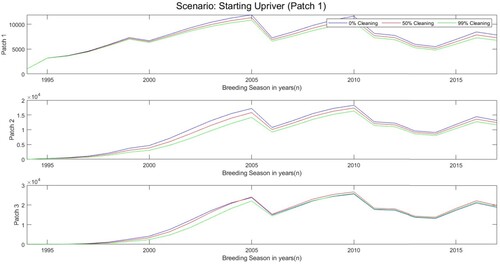
Table 6. Spread of zebra mussels from upriver (patch1) using the two-way movement of the three patch model. Cleaning factors were added to the spread of zebra mussels from upriver. The initial number of juveniles, small adults, and large adults in year 1994 are 5, 489, and 503, respectively. Table results refer to the year 2017.

Two-Way Movement starting in Patch 1
	Upriver	Midriver	Downriver	Combined
J	5,425	9,938	16,303	31,666
$A_a$	1,652	2,465	3,319	7,436
$A_b$	754	808	842	2,404
Total	7,831	13,211	20,464	41,506
Added Cleaning Factor of 0.5
J	5,044	9,358	15,754	30,156
$A_a$	1,538	2,325	3,237	7,100
$A_b$	697	758	809	2,264
Total	7,279	12,441	19,800	39,520
Increased Cleaning Factor to 0.99
J	4,683	8,786	15,278	28,747
$A_a$	1,430	2,187	3,160	6,777
$A_b$	644	709	791	2,144
Total	6,757	11,682	19,229	37,668

5.2. Scenario 2: spread starting downriver

In another effort to better highlight the possible role of effective boat cleaning, we investigate the scenario of zebra mussels starting in the downriver patch, i.e. patch 3. Since zebra mussels are able to move from patch to patch following the natural river flow downstream, by showing this scenario, we can avoid the possibility of the downriver dispersal by natural river flow negating the effect of boat cleaning. We only focussed on two-way boat movement. Assume that in patch 3, there were 34 juveniles, 2, 059 small adults, and 3, 092 large adults, per square metre, and that no zebra mussels in patches 2 and 3 in the year 1994. In Table 7, we can see the total number of zebra mussels and the effect of the cleaning factors. Starting downriver leads to fewer zebra mussels, and the cleaning factors have more effect on the percentage of zebra mussel population compared to Scenario 1. The cleaning factor of 0.5 decreased the number of zebra mussels by about $6.3\mathrm{\%}$ and the cleaning factor of 0.99 decreased the number of zebra mussels by about $32.9\mathrm{\%}$. Figure 9 shows the population size in the patches through time when there was a cleaning factor of $0\mathrm{\%}$, $50\mathrm{\%}$, or $99\mathrm{\%}$.

Figure 9. Population size of zebra mussels from 1994 to 2017 with a cleaning factor of either $0\mathrm{\%}$, $50\mathrm{\%}$, or $99\mathrm{\%}$. Scenario starting in patch 3 (downriver) where the initial number of juveniles, small adults, and large adults in year 1994 are 34, 2, 059, and 3, 092, respectively.

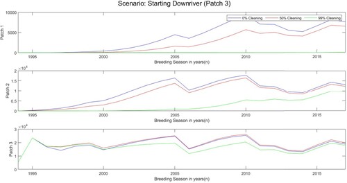
Table 7. Spread of zebra mussels from downriver (patch3) using the three patch two-way movement model. Cleaning factors were added to restrict the spread of zebra mussels from upriver. The initial number of juveniles, small adults, and large adults in year 1994 are 34, 2, 059, and 3, 092, respectively. Table results refer to the year 2017.

Two-Way Movement starting in Patch 3
	Upriver	Midriver	Downriver	Combined
J	5,290	9,886	16,154	31,330
$A_a$	1,612	2,453	3,309	7,374
$A_b$	740	806	818	2,364
Total	7,642	13,145	20,281	41,068
Added Cleaning Factor of 0.5
J	4,506	9,211	15,672	29,389
$A_a$	1,378	2,293	3,224	6,895
$A_b$	639	751	808	2,198
Total	6,523	12,255	19,704	38,482
Increased Cleaning Factor to 0.99
J	39	7,104	14,177	21,320
$A_a$	13	1,810	2,988	4,811
$A_b$	7	621	782	1,410
Total	59	9,535	17,947	27,541

5.3. Scenario 3: increasing parameters(Survival proportion & movement)

This scenario presents the effect that increasing parameters have on the spread of zebra mussels starting from either patch 1 or patch 3. We begin by increasing the survival proportion by multiplying original survival proportion by 1.1. With the increase in survival proportions, there were a higher number of zebra mussels in each patch. However, since survival proportions were increased, the effectiveness of the cleaning factors was lower, as we can see in Table 8. On the other hand, increasing movement rates by multiplying original movement rates by 5 resulted in higher percent decreases in total population size for both the scenario starting in patch 1 and the scenario starting in patch 3.

Table 8. Percent decrease in population sizes with larger survival proportions and movement rates in the three patch model with two-way movement with either a $50\mathrm{\%}$ or a $99\mathrm{\%}$ cleaning factor.

Starting in Patch 1
	Original	Increased	Increased
%Decrease	Parameters	Survival proportions	Movement proportions
Original to $50\mathrm{\%}$ cf	4.8%	4.0%	27.1%
Original to $99\mathrm{\%}$ cf	9.2%	7.7%	57.4%
Starting in Patch 3
	Original	Increased	Increased
%Decrease	Parameters	Survival proportions	Movement Rates
Original to $50\mathrm{\%}$ cf	6.3%	4.3%	27.1%
Original to $99\mathrm{\%}$ cf	32.9%	28.2%	70.7%

6. Discussion and conclusions

We used continuous and discrete-time equations, to represent the different temporal dynamics of the larvae class and the juvenile, small adult, and large adult classes, respectively. We illustrated the effect of temperature and density-dependent survival on the population growth of zebra mussels. By using Hudson River data, a one patch model was first examined to showcase zebra mussels' life cycle and population growth from the year 1994 to 2017. This model was then expanded to look at the movement between three locations or successive patches (upriver, midriver, and downriver). Movement was observed by using flow driven movement (one-way movement) and by using boat movement in addition to the natural river flow (two-way movement). For the three patch models, we assumed that no new zebra mussels entered the system outside the three patches and that no zebra mussels left the three patches.

For the one patch and the three patch models, we were able to obtain some parameters from literature but also had to do parameter estimation for other unknown parameters (see Table 4) via MATLAB tools MultiStart and fmincon. We tried to obtain oscillations and an approximate fit to the data from the Hudson River, which is obviously not a closed system and whose data were also limited. Since our system is a closed system (no input or outflow), we investigated whether the mussel population would persist and how they spread in such a habitat. A more detailed fitting of parameters with confidence intervals is beyond the scope of our current work and data. With these parameters, we were able to observe realistic population growth and population spread. We were also able to determine the stability of the one patch model and three patch model with two-way movement and the net reproductive number of the one patch model. We noticed that if the reproduction rates of adults. $r_a$ and $r_b$ were large enough, that the zero solution would be an unstable equilibrium in both models (one patch and three patches), and the numerical value of the net reproductive number (for our parameters) can become greater than one, which results in the zebra mussel population increase over time. Once these models were formulated and analyzed, we specifically focussed on the three patch model with two-way movement to run different scenarios and found that boat and natural river movement increased zebra mussel spread. Spread was observed from two different starting locations. By only having zebra mussels starting in one location at a time, we were able to see how zebra mussels moved through the three patches coming from either upriver or downriver.

Cleaning factors were multiplying the movement rates to slow down the spread when a boat enters a new patch. These cleaning factors could be cleaning or inspecting boats before they enter a new location. Depending on the cleaning factor, zebra mussel spread decreased over the total years of our study. We looked at a cleaning factor where only $50\mathrm{\%}$ of the boats that entered new locations were cleaned. To expand our study we also looked at the impact of cleaning $99\mathrm{\%}$ of the boats that entered new locations, but that is a bit unrealistic. Unfortunately, only cleaning half the boats that enter locations does not prevent zebra mussels from growing or spreading on those boats that were not cleaned. This result reinforces the well-established idea in invasion biology that it is often more effective to prevent an invasion than to control the spread and population growth of an invader after it is established [1, 15].

In an attempt to see the different effects of cleaning, we increased the survival proportions and movement rates of the three patch model with two-way movement. The results showed that increasing survival proportions decreased the effectiveness of the cleaning factors while increasing the movement rates drastically increased the effectiveness of the cleaning factors. Overall, the scenario of starting in patch 3 with a cleaning factor of $99\mathrm{\%}$ and increased movement rates efficiently decreased the number of zebra mussels. Therefore, if we could improve cleaning methods and the number of boats cleaned, we could decrease the amount of spreading to other locations.

Our results indicate changes in certain survival proportions or movement rates can force $R_0$ to decrease, which is important. Cleaning can affect some rates to slow the spread with a small effect, therefore more research work is needed on how to prevent an invasion.

Disclosure statement

No potential conflict of interest was reported by the author(s).

Additional information

Funding

Collection of Hudson River data was supported by grants from the National Science Foundation and the Hudson River Foundation.

References

- D.A. Ahmed, E.J. Hudgins, R.N. Cuthbert, M. Kourantidou, C. Diagne, P.J. Haubrock, and F. Courchamp, Managing biological invasions: the cost of inaction, Biol. Invasions. 24 (2022), pp. 1927–1946.
- L.J.S. Allen and P. van den Driessche, The basic reproduction number in some discrete-time epidemic models, J. Differ. Equations Appl. 14 (2008), pp. 1127–1147.
- A.J. Benson, D. Raikow, J. Larson, A. Fusaro, A.K. Bogdanoff, and A. Elgin, Dreissena polymorpha (Pallas, 1771): U.S. Geological Survey, Nonindigenous Aquatic Species Database, 2022. Available at https://nas.er.usgs.gov/queries/factsheet.aspx?speciesID=5 (accessed: 07.24.2022).
- Cary Institute of Ecosystem Studies, Environmental Monitoring Program, 1988. Available at https://www.caryinstitute.org/science/research-projects/environmental-monitoring-program/weather-climate (accessed: 06.28.2022).
- Cary Institute of Ecosystem Studies, Zebra Mussel Fact Sheet, 2020. Available at https://www.caryinstitute.org/news-insights/2-minute-science/zebra-mussel-fact-sheet (accessed: 11.05.2020).
- N.A. Connelly, C.R O'Neil, B.A. Knuth, and T.L. Brown, Economic impacts of zebra mussels on drinking water treatment and electric power generation facilities, Environ. Manage. 40 (2007), pp. 105–112.
- J.M. Cushing, An Introduction to Structured Population Dynamics, Society for Industrial and Applied Mathematics, 1998.
- M. Czarnoleski and T. Muller, Antipredator strategy of zebra mussels (dreissena polymorpha): from behavior to life history, in Quagga and Zebra Mussels: Biology, Impacts, and Control, Taylor & Francis Group, Boca Raton, FL, 2014, pp. 345–357.
- D.W. Garton, R. McMahon, and A.M. Stoeckmann, Limiting environmental factors and competitive interactions between zebra and quagga mussels in North America, in Zebra and Quagga Mussels: Biology, Impacts, and Control, 2nd ed., CRC Press, Boca Raton, 2014, pp. 383–402.
- S.N. Higgins and M.J. Vander Zanden, What a difference a species makes: a meta-analysis of dreissenid mussel impacts on freshwater ecosystems, Ecol. Monogr. 80 (2010), pp. 179–196.
- Q. Huang, H. Wang, and M.A. Lewis, A hybrid continuous/ discrete-time model for invasion dynamics of Zebra mussels in rivers, SIAM J. Appl. Math. 77 (2017), pp. 854–880.
- Y. Jin and X.Q. Zhao, The spatial dynamics of a Zebra mussel model in river environments, Discrete Continuous Dyn. Syst. Ser. B 26 (2021), pp. 1991–2010.
- J. Kobak, Behavior of Juvenile and adult zebra mussels (Dreissena polymorpha), in Quagga and Zebra Mussels: Biology, Impacts, and Control, Taylor & Francis Group, Boca Raton, FL, 2014, pp. 331–344.
- Lake Winnipeg Foundation, Zebra Mussels 101, 2022. Available at https://lakewinnipegfoundation.org/zebra-mussels-101 (accessed: 11.05.2022).
- B. Leung, D.M. Lodge, D. Finnoff, J.F. Shogren, M.A. Lewis, and G. Lamberti, An ounce of prevention or a pound of cure: bioeconomic risk analysis of invasive species, Proc. Royal Soc. London. Ser. B: Biological Sciences 269 (2002), pp. 2407–2413.
- L. Mari, E. Bertuzzo, R. Casagrandi, M. Gatto, S.A. Levin, I. Rodriguez-Iturbe, and A. Rinaldo, Hydrologic controls and anthropogenic drivers of the zebra mussel invasion of the Mississippi-Missouri river system, Water. Resour. Res. 47 (2011), pp. 1–16.
- MathWorks, Constrained Nonlinear Optimization Algorithms, 2022. Available at https://www.mathworks.com/help/optim/ug/constrained-nonlinear-optimization-algorithms.html (accessed: 01.26.2022).
- MathWorks, How GlobalSearch and MultiStart Work, 2022. Available at https://www.mathworks.com/help/gads/how-globalsearch-and-multistart-work.html (accessed: 01.26.2022).
- MathWorks, MATLAB, 2022. Available at https://www.mathworks.com/products/matlab.html (accessed: 01.26.2022).
- MathWorks, What Is Global Optimization?, 2022. Available at https://www.mathworks.com/help/gads/what-is-global-optimization.html (accessed: 01.26.2022).
- New Hampshire Department of Environmental Services, Environmental Fact Sheet, 2019. Available at https://www.des.nh.gov/sites/g/files/ehbemt341/files/documents/2020-01/bb-17.pdf (accessed: 11.05.2020).
- A.B. Potapov and M.A. Lewis, Allee effect and control of lake system invasion, Bull. Math. Biol. 70 (2018), pp. 1371–1397.
- D.L. Strayer, B.V. Adamovich, R. Adrian, D.C. Aldridge, C. Balogh, L.E. Burlakova, H.B. Fried-Petersen, L. G.-Tóth, A.L. Hetherington, T.S. Jones, A.Y. Karatayev, J.B. Madill, O.A. Makarevich, J.E. Marsden, A.L. Martel, D. Minchin, T.F. Nalepa, R. Noordhuis, T.J. Robinson, L.G. Rudstam, A.N. Schwalb, D.R. Smith, A.D. Steinman, and J.M. Jeschke, Long-term population dynamics of dreissenid mussels (Dreissena polymorpha and D. rostriformis): a cross-system analysis, Ecosphere 10 (2019), p. e02701.
- D.L. Strayer, D.T. Fischer, S.K. Hamilton, H.M. Malcom, M.L. Pace, and C.T. Solomon, Long-term variability and density dependence in Hudson river dreissena populations, Freshwater Biol. 65 (2020), pp. 474–489.
- D.L. Strayer and H.M. Malcom, Long-term demography of a zebra mussel (Dreissena polymorpha) population, Freshw. Biol. 51 (2006), pp. 117–130.
- H.R. Thieme, Spectral bound and reproduction number for infinite-dimensional population structure and time heterogeneity, SIAM. J. Appl. Math. 70 (2009), pp. 188–211.
- Weather Underground, Latham, NY Weather History (Albany International Airport Station), 1988. Available at https://www.wunderground.com/history/daily/us/ny/albany/KALB (accessed: 06.28.2022).
- J.D. White, S.K. Hamilton, and O. Sarnelle, Heat-induced mass mortality of invasive zebra mussels (Dreissena polymorpha) at sublethal water temperatures, Can. J. Fisheries Aquatic Sci. 72 (2015), pp. 1221–1229.