Movement analysis with inertial sensors: identification of noise covariance matrices to improve body segment orientation using Kalman filtering

Keywords:

• Motion analysis
• Inertial measurement unit
• Kalman filter
• covariance matrix

1. Introduction

In the fields of medicine and biomechanics, human motion analysis is used to extract quantitative and objective data to characterize a movement. Human motion analysis is now mainly based on optoelectronic systems measuring 3D coordinates of reflective markers. But such systems suffer from two main drawbacks:

(1)	They are heavy systems, difficult to move to different places of experimentation.
(2)	Measurement is restricted to camera’s field of vision.

In this context, inertial measurement units (IMU) are a promising way to perform human motion analysis out of the lab, with no need for external devices.

However, IMUs do not measure directly the orientation but only acceleration, rotation rate, and magnetic field. These data have thus to be converted in order to estimate the orientation. Moreover, IMUs designed for human motion analysis are based on MEMS technology which allows sensors to be cheap and small but which also induces noise and bias over the measurement.

In the literature, Kalman filtering is recognized as one of the best tool to perform data fusion from noised measurement. The main idea is to combine the sensors measurement with a dynamic model that translates the time-behaviour of the state to be estimated.

However, there is no consensus on the structure of the algorithm and its settings. A critical point when implementing a Kalman filter is the definition of the two covariance matrices that characterize mismodelling and input error from noisy sensors. There is no consensus in the literature on a method to define these covariance matrices, even if it is crucial since it can lead to inaccurate estimation as well as divergence and stability problems (Foxlin 1996).

The aim of this study is to provide a solution to identify input parameters that optimize orientation estimation.

2. Methods

In order to identify the optimal set of parameters for inertial measurement, we used an optoelectronic system as a reference. Both systems recorded simultaneously the orientation of an object moved by hand.

2.1. IMU processing

In this study, the orientation was successively computed from three IMUs (Opal sensors, APDM, Portland, OR). Sensors data (triaxial accelerometers, gyroscopes and magnetometers) were collected at 128 Hz and fused in a custom Kalman filter.

As the measurement model that relates sensors data to the orientation (expressed as a quaternion) is non-linear, we built an Extended Kalman Filter (EKF). To facilitate quaternion computation and to lighten the state vector, we privileged a multiplicative indirect Kalman structure (Trawny & Roumeliotis 2005). The state vector was augmented with gyroscopes bias whose behaviour was modelled as a random walk. Rates of rotation were thus corrected before the numerical integration.

2.2. Gold standard measurement

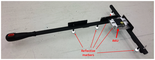
In order to assess the accuracy of IMU estimation, we used an optoelectronic measurement (VICON system, 20 cameras, 250 Hz) considered as the gold standard in biomechanics. The object of interest, initially equipped with an IMU, was thus fitted with five reflective markers (Figure 1).

Figure 1. Object equipped with both an IMU and five reflective markers.

2.3. Imposed movements

As the parameters to be identified characterise sensor errors that are not taken into account by calibration (like non-linearity, hysteresis or g-sensitivity), it can be envisaged that their values depend on the nature of the movement. In this study, movements were imposed by hand at three different levels of intensity during ten minutes. The Table 1 lists the main kinematic characteristics of these three imposed movements.

Table 1. Main kinematic characteristics of the imposed movements.

Intensity	Slow	Inter.	Rapid
Acceleration (g)	0.03 ± 0.02	0.7 ± 0.5	4 ± 2
Rate of rotation (deg/s)	40 ± 20	300 ± 150	700 ± 400

2.4. Parameters identification

The 3 IMUs were tested at the 3 levels of intensity previously defined. The experimentation was repeated 3 times during 3 consecutive days.

The process $\mathit{Q}$ and measurement $\mathit{R}$ covariance matrices can be defined as follows:(1) $$\mathit{Q}={\mathit{\sigma }}_g·{\mathit{I}}_3$$(1) (2) $$\mathit{R}=\left[\begin{array}{cc}{\mathit{\sigma }}_a·{\mathit{I}}_3& 0_3\\ 0_3& {\mathit{\sigma }}_m·{\mathit{I}}_3\end{array}\right]$$(2)

From this assumption, σ_g, σ_a and σ_m, that denote respectively the gyroscopes, accelerometers and magnetometers measurement error, are the three parameters to be identified.

After selecting a set of ten values per parameter, the orientation were computed by the Kalman filter for the thousand possible combinations. Each time, the RMS of the error calculated with respect to the optoelectronic measurement was calculated as follows:(3) $$d\overline{q}={\overline{q}}_{IMU}\otimes {\overline{q}}_{opto}^{\ast }$$(3) (4) $$\mathit{\theta }=2·acos\left(d{\overline{q}}_4\right)$$(4)

The error can thus be represented on a graph as a surface against σ_g and σ_a. Then, the effect of the magnetometers on the error can be seen by scrolling the graph for the different values of σ_m. Finally, the optimal set of parameters can be identified at the minimal error point.

3. Results and discussion

Common results lead to a valley when representing the error against σ_g and σ_a (Figure 2). There is thus a proportionality law that link the optimal values for these two parameters. Then, when looking at the influence of magnetometers, the surface leads generally to an optimal point.

Figure 2. RMS of the error against accelerometers and magnetometers uncertainties.

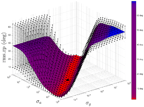
Figure 2 shows that a bad parameter choice can induce a huge error (up to 60° for this movement), the proposed protocol is thus essential. For the three tested sensors, the optimal parameters lead to errors of about 1.5°, 3° and 13.5° for slow, intermediate and rapid movements respectively.

It should be kept in mind that the rapid movement corresponds to the worse conditions that could be faced in a real human task: very intensive motion with no rest period. Common movements are generally a mix of accelerations and rest periods (like stance and swing phases during gait) which allows gyroscopes bias to be frequently corrected. These results are thus acceptable for most of the studied human motions.

4. Conclusions

The presented method gives a solution to identify the optimal covariance matrices values for Kalman filtering. Moreover, the proposed visualization of the error allow to better ‘see’ many parameters influence on the algorithm behaviour.

Acknowledgements

This work has been sponsored by the French government research program ‘Investissements d’Avenir’ through the Robotex Equipment of Excellence.

References

- Foxlin E. 1996. Inertial head-tracker sensor fusion by a complementary separate-bias Kalman filter. VR Annu Int Symp Proc IEEE 1996. p. 185–194, 267.
- Trawny N, Roumeliotis SI. 2005. Indirect Kalman filter for 3D attitude estimation. University of Minnesota. Technical Report 2005-002.