Locating and sizing tumor nodules in human prostate using instrumented probing – computational framework and experimental validation

Abstract

Detection of tumor nodules is key to early cancer diagnosis. This study investigates the potential of using the mechanical data, acquired from probing the prostate for detecting the existence, and, more importantly, characterizing the size and depth, from the posterior surface, of the prostate cancer (PCa) nodules. A computational approach is developed to quantify the uncertainty of nodule detectability and is based on identifying stiffness anomalies in the profiles of point force measurements across transverse sections of the prostate. The capability of the proposed method was assessed firstly using a ‘training’ dataset of in silico models including PCa nodules with random size, depth and location, followed by a clinical feasibility study, involving experimental data from 13 ex vivo prostates from patients who had undergone radical prostatatectomy. Promising levels of sensitivity and specificity were obtained for detecting the PCa nodules in a total of 44 prostate sections. This study has shown that the proposed methods could be a useful complementary tool to exisiting diagnostic methods of PCa. The future study will involve implementing the proposed measurement and detection strategies in vivo, with the help of a miniturized medical device.

Keywords:

• Inverse problem
• Prostate cancer
• Tumor detection
• Tissue mechanics

1. Introduction

Detection of tumor nodules is the key to early cancer diagnosis. For prostate cancer (PCa), first indications are usually a raised level of prostate-specific antigen (PSA) in the blood, supplemented by digital rectal examination (DRE), which involves palpation of the accessible surface of the prostate through the rectum. There is a continuing clinical need to improve both sensitivity and specificity of simple early screening methods, to better stratify risk for further diagnostic steps such as magnetic resonance imaging (MRI), transrectal ultrasound (TRUS) and biopsy. Recent research has seen increasing interest in instrumenting prostate gland palpation, either for the purpose of enhancing DRE (Kim et al. 2014; Scanlan et al. 2015; Palacio-Torralba et al. 2016) or minimally invasive robot-assisted surgery (Li et al. 2017). The data acquired from such methods are often in the format of force feedback when probing the prostate, either quasi-statically or dynamically, and integrating such strategy of data analysis into DRE procedures has shown promise for improving the effectiveness of early screening for PCa (Hammer et al. 2017). This has been based on observations that cancerous tissue has a higher elastic modulus (Krouskop et al. 1998; Phipps et al. 2005; Carson et al. 2011) than, and different viscoelastic behaviors (Palacio-Torralba et al. 2015; Baghban and Mojra 2018; Yang et al. 2018) from, its healthy counterpart in many tissue types including prostate, breast and pancreas, thus making it possible to detect the tumor nodules based on mechanical measurement.

Despite the above, largely empirical, developments in prostate probing for tumor detection, it is still challenging to extract key information about PCa nodules (e.g., location and volume) from the mechanical data, particularly at the early stages where little supplementary information, such as the size of the prostate, are known. Most previous studies required a priori knowledge of the geometries of the prostate and PCa nodules as well as their mechanical properties, which would limit their practical use. Among the limited number of existing studies that are capable of detecting and characterizing PCa nodules using probing, Liu et al. (2014) modelled a rolling indentation probe and proposed an inverse finite element method to estimate the depth of the PCa nodule. Methods such as artificial neural networks have also been exploited to predict the elasticity of cancerous nodules in soft tissue along with their depth and size (Hosseini et al. 2007; Keshavarz and Mojra 2015; Nichols and Okamura 2015). These and other approaches, despite of their usefulness, often require a priori knowledge of the presence of PCa nodule, the mechanical properties of the tissues and the stress or strain field in the prostate under deformation, which is usually incompatible with data obtained from mechanical probing.

Detecting the size and location of tumor nodules in soft tissue using the mechanical measurements made at its boundary is challenging due to its mathematically-ill-posed nature and uncertainty. Unlike its ‘forward problem’ that is usually deterministic, such an inverse problem may involve a high level of uncertainty given rise by a multitude of parameters, most notably the size, depth (distance from the boundary where measurements are made) and the ‘contrast’ in mechanical properties between the tumor nodule and its surroundings. For example, a small tumor nodule near the surface could lead to similar mechanical measurement data compared to that from a larger and more distant nodule. Such ambiguity needs to be tackled by a strategy with an aim of reducing, if not completely eliminating, the uncertainty so that the size and depth of the tumor nodule can be confidently characterized. As a result, this study aims to establish a model-informed framework, based on the mechancial chacaterization data from the tissue surface, to detect the existence, and characterize the size and depth, of stiff cancerous nodules in soft tissue.

2. Methods

2.1. Patient group selection and rationale

This study investigates the potential of using the force measurement data, acquired from probing the prostate, as the sole means of detecting the existence and characterizing the size and depth of the PCa nodules, with the ultimate goal of establishing a quantitative framework for enhancing the sensitivity and specificity for clinical applications such as in situ tumor nodule detection. To this end, an ex vivo study (full ethics approval granted by NHS Regional Ethics Committee − 12/SS/0148) was carried out on whole prostates following radical prostatectomy, to demonstrate an early-stage validation towards a future in vivo study. This made it possible to carry out the mechanical measurements at multiple locations over the posterier surface, mimicking a clinically-relevant DRE procedure, and to acquire cross-prostate histology slices for validating the detection outcomes such as the size and location of tumor nodules.

2.2. Instrumented probing and histology study

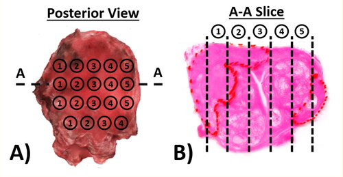
The experimental and histology sectioning protocol, as shown in Figure 1, was based on the one used for a wider study (Hammer et al. 2017) of patients who were scheduled for radical prostatectomy. The mechanical measurements were conducted immediately after the prostate was removed from the patient. It included a 10 N load cell (miniature in-line, Omega Engineering) and a rigid probe, hemispherical and 2 mm in diameter, was driven down towards the posterior surface of the prostate using a loading stage with three-dimensional motion control. After the contact between the probe and the posterior surface of the prostate was identified with an approach speed (0.1 mm/s), a vertical displacement of 8 mm with a speed of 0.5 mm/s was then applied along the posterior-anterior direction and the force feedback was recorded. The indentation speed was kept as low as practically possible to minimise the effect of viscoelastic behavior of the prostate tissue. The maximum displacement of 8 mm was chosen based on a number of considerations: 1) a limited depth that causes no tissue damage to the prostate specimen; 2) potential future application of in vivo trans-rectal measurements, although the intrinsic tension of the rectal wall may cause a much higher force needed to reach the same indentation depth in comparison to the current ex vivo study; and 3) in line with our findings from a previous finite-element study (Palacio-Torralba et al. 2015) where 8 mm was found to be sufficient to ‘detect’ the prostate through the rectal wall. The peak force at the maximum indentation depth was recorded at an array of probe points, spaced at a minimum of 6 mm apart, as illustrated in Figure 1. Since the scope of this study remains within the quasi-static/quasi-elastic regime, the consideration here is to minimize the effect of the viscoelasticity, or more generally irreversible effects such as tissue visco-elasto-plasticity, which would lead to the indentation being affected by a previous, adjacent, measurement. The minimum distance of 6 mm between adjacent probing points was therefore chosen to reach a trade-off between the ‘quasi-elastic’ consideration mentioned above and the practical consideration where the aim was to achieve as many probing points as possible on the prostate surface (usually in a few cm × cm). After the measurement, surgical clips were placed in each row to allow the histological sections to be registered to the probe points. Transverse sections through each row were prepared and stained using the standard H&E (hematoxylin and eosin) technique, followed by patho-histological examination, where the outlines of the PCa nodules were drawn by a consultant uropathologist.

Figure 1. Experimental and sectioning methods. The prostate specimen is mechanically characterized following radical prostatactomy. A) The prostate posterior surface was marked with surgical clips to register the probing points and histological sections; and B) typical histological mega-slice showing columns under probe points, where the boundaries of the PCa nodules were drawn by the uropathologist.

A total of 13 prostates were included in this study, each having between 36 and 42 probing points, leading to a total of 44 histological slices along the left-right axis. All histological slices were converted into finite element models, where the outlines of the prostate and PCa nodules were preserved and compared with the detection outcomes.

2.3. The prostate models and patient data

2.3.1. In silico model

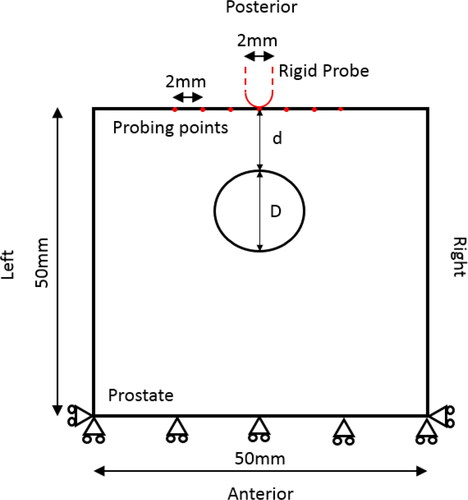
Figure 2 illustrates the simplified in silico model, represented by a ‘square box’ of 50 × 50 mm, the upper side being the posterior surface, where the probing was carried out. The model was constrained at the anterior surface, as shown, to reproduce the experimental indentation measurements.

Figure 2. Schematic of simplified 2D prostate model with a single PCa nodule embedded in it.

2.3.2. Finite element modelling

For the in silico Finite Element (FE) model, point-wise probing was simulated, where the probe was modelled as a rigid hemisphere, 2 mm in diameter, in line with the experimental configurations. Accordingly, probing points were spaced 2 mm apart and the force recorded at a depth of 8 mm for each point. The contact with the soft tissue was assumed to be frictionless (Ahn and Kim 2009) and the point-by-point probing was considered to be quasi-static, using a strain rate lower than 0.01 s⁻¹, again in line with the experimental parameters, allowing the soft tissue to be modelled as a hyper-elastic material (Cox et al. 2008). A nearly-incompressible (Miller 2005) neo-Hookean hyperelastic model was used, whose strain energy function can be expressed as (1) $$W=\mathrm{}{C}_1\left({\overline{I}}_1-3\right)+\frac{1}{D_1}\mathrm{}{\left(J-1\right)}^2$$(1) (2) $${\overline{I}}_1=J^{-\frac{2}{3}}\mathrm{}{I}_1,\mathrm{}{\mathrm{}D}_1=\mathrm{}\frac{2}{K_0}=\mathrm{}\frac{3\mathrm{}(1-2v)}{{\mu }_0\mathrm{}(1+v)}\mathrm{}\mathit{and}\mathrm{}{\mu }_0=2C_1$$(2) where ${\overline{I}}_1$ the first strain invariant of the left Cauchy-Green deformation tensor and $J$ the determinant of the deformation gradient. The remaining material parameters, $C_{1\mathrm{}}{D}_1,$ are related to bulk modulus ($K_0$), initial shear modulus (${\mu }_0$) and Poisson’s ratio ($\nu$). To the best knowledge of the authors, there is no direct, well defined, mechanical measurements on human prostate tissues (both healthy and PCa) with reported hyperelastic parameters available in literature. Therefore the approach taken here was to fit the hyperelastic model above to the published elasticity data adopted from the work by Hoyt et al. (Hoyt et al. 2008), who measured the Young’s moduli of the non-cancerous and cancerous tissues from ex vivo radical prostatectomy samples as 17 kPa and 42.5 kPa, respectively. The Poisson’s ratio of both tissue types was taken to be 0.49 (Torlakovic et al. 2005). The resulting neo-Hookean model in Eq. (1)(1) $$W=\mathrm{}{C}_1\left({\overline{I}}_1-3\right)+\frac{1}{D_1}\mathrm{}{\left(J-1\right)}^2$$(1) was characterised to have C₁ =2.85 kPa and D₁ = 7067 kPa for non-cancerous tissue and C₁ = 7.12 kPa and D₁ = 2827 kPa for PCa tissue. The FE models were meshed with four-node bilinear plane stress quadrilateral elements (mesh refinement was conducted to ensure cost-effective convergence) and solved in ABAQUS (v6.14, Dassault Systemes, Vlizy Villacoublay, France).

2.4. A probabilistic approach to PCa detection

Due to the ill-posed nature of the inverse problem, a certain set of force measurements on a prostate surface could, in principle, arise from an infinite number of arrangements of PCa nodules of a higher stiffness distributed in a surroudning matrix of lower stiffness. To tackle this uncertainty, the methodology taken here is to generate a series of probability functions for size and position of nodules and to match these with the observed profile in order to detect the nodules in a probabilistic approach.

2.4.1. The force profile

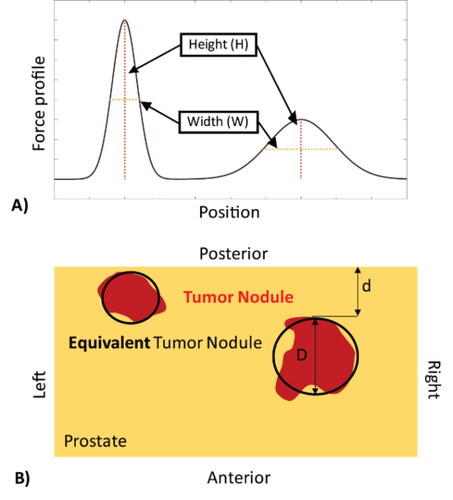
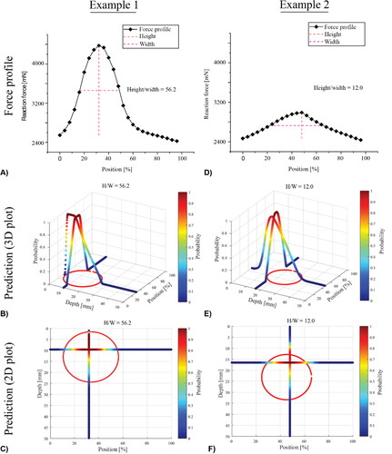
For each postulated nodule size and location, simulated forces at the 8 mm indentation depth were determined at each probing point, to obtain force profiles along the surface of the ‘slice section’ over the posterior surface of the prostate. Each individual force profile, for example Figure 3, has a characteristic set of local peaks, influenced by inhomogeneities given rise by the presence of a stiff PCa nodule (Sangpradit et al. 2011). Furthermore, one can imagine that a peak in the force profile would be sensitive to the size and depth of any PCa nodule, becoming ‘sharper’, i.e., taller and narrower, when the nodule is located near the posterior surface (i.e., closer to the probe) and/or is of a larger volume. Therefore, the peak sharpness, represented by the ratio between peak height and width was chosen as a feature, the width being defined by the y-coordinates where the forces drops to half of its maximum height (Figure 2). It is worth highlighting that, since both the size and depth of the PCa nodule could influence the peak force in a similar way – a larger and deeper nodule may lead to a similar peak to one caused by a smaller but shallower nodule therefore, as aforementioend, a probabilistic approach with uncertainty quantification needs to be taken.

Figure 3. Example of simulated force profile from point probing. A) Two peaks can be identified, each having a different height and width characteristic; and B) the corresponding prostate model, in which the red areas denote the cancerous nodules and the black outlines indicate the predicted nodule characteristics. d: nodule depth; D: nodule size.

2.4.2. Random datasets

The approach here is to ‘search’ the peak in the experimental force profile amongst 2500 postulated force profiles, generated by randomly assigning a single PCa nodule with varying sizes (between 2 mm and 24 mm in diameter) and depths (between 2 mm and 30 mm), in the in silico prostate model. Specifically, the range of PCa nodule diameter in the randomly-generated models was derived from the entire dataset of this study where all PCa nodules from the histological slides had an area between 3 ∼ 450mm², equivalent to a diameter range of 2 ∼ 24mm. The resulting peak was then characterized by its height-by-width (H/W) ratio. Figure 4 shows a clear trend of positive correlation between this ratio and the ‘power of influence’, i.e., the diameter and depth of the nodule (D/2d), in the peak profile caused by the PCa nodule. This means that, the larger and shallower the nodule is, the sharper the peak becomes. Interestingly, the span of data, which is a measure of the uncertainty in such correlation, increases significantly when the peak becomes sharper. For flatter peaks, i.e., those with smaller H/W values, almost all simulated PCa nodules are located deeply in the prostate (i.e., greater value of depth, D), regardless of their sizes. However, when the peak becomes sharper, either small nodules with very shallow depth or larger but deeper nodules could lead to similar peaks, leading to greater dispersion and uncertainty.

Figure 4. Correlation between the peak sharpness (H/W) and the nodule radius/depth (D/2d), of all random models (excluding those with unidentifiable peaks with H/W<5). Using the peak sharpness, H/W, the entire dataset is divided into 6 groups, each having characteristic probability distribution of the corresponding nodule size and depth. All these characteristic probability distributions can be employed to identify the PCa nodule, using the methodology described in Electronic Supplementary Materials.

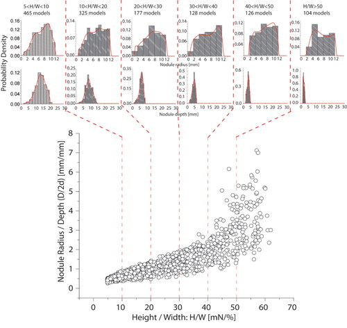
For a given peak with a certain sharpness value (x-axis in Figure 4), the size-to-depth ratio of the corresponding tumor nodule falls into the range (along the y-axis) depicted by the random representative models. To implement this, the entire random dataset was divided into 6 groups according to their values of peak sharpness, namely, 5-10 (465 cases), 10-20 (325cases), 20-30 (177 cases), 30-40 (128 cases), 40-50 (126 cases), higher than 50 (104 cases), as shown by the vertical dashed lines in Figure 4. It is worth noting that Figure 4 does not include 1175 cases where the sharpness value is less than 5, below which a peak in the force profile cannot be considered to be sensitive to the presence of a PCa nodule (either too small or too deep). Each of the six groups has associated size and depth ranges to the corresponding PCa nodule, approximated by the histograms in Figure 4. The histograms for nodule depth are narrow and the modal/peak values are sensitive to H/W, meaning that depth can be estimated with less uncertainty than size.

The probabilistic methods of uncertainty quantification proposed in this study are included in Appendices A and B, where steps for tumor nodule detection and predicting the probabilities along both anterior-posterior and left-right axes are presented.

3. Sensitivity analysis with simplified prostate models

3.1. Detecting single tumor nodules

To demonstrate the probabilistic approach and its sensitivity, the force profiles for 400 models, of the type illustrated in Figure 2, with random values of size and depth for a single PCa nodule, were generated as a test set. The proposed methods were used to predict the sizes and locations of the embedded single PCa nodules.

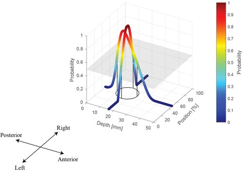
Figure 5 shows two representative cases, both having nodules of similar diameter (D₁=22.8 mm; D₂=20.6 mm) but with very different depths (d₁=1.5 mm; d₂=13mm). In both cases, the peak in the force profile was identified and characterized, as shown in Figure 5 (A) and (D). The locations of the two nodules (red circles) and the probabilities in the axial and depth directions are also displayed. It can be seen that, since the nodule is located more deeply in case 2, its peak value is much lower and force profile is less sharp (H/W = 12, in comparison with the H/W = 56.2 in case 1). This has also led to two distinct predictions, as shown in Figure 5C and F. Interestingly, for the shallow PCa nodule in Case 1, the prediction map has a large area that has probabilities close to ‘1′, i.e., a high level of prediction certainty, near the centre of the nodule, particularly along the anterior-posterior axis. Although the detection also correctly captures the nodule location for case 2, it has a much smaller area with probabilities close to ‘1′, indicating a lower degree of certainty.

Figure 5. Two examples of simplified prostate models, including the force profile and the predictions in 3D and 2D with illustrated probabilities.

To quantify this further, a threshold of acceptable detectability is introduced to the probability values across both the anterior-posterior and left-right axes. Such a threshold can be visualised, as a plane in the depth-position axes, above which a binary prediction can be made. The effect of the chosen probability threshold on the prediction outcome is demonstrated in Electronic Supplementary Material (ESM 1).

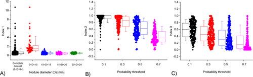
To assess the effectiveness of the proposed method in predicting the PCa nodules in all 400 random models, three indices are used here: (3) $${\mathrm{I}}_1=\mathit{dist}\left(C_{p,}\mathrm{}{C}_{TN}\right)/(D/2)$$(3) (4) $${\mathrm{I}}_2=A_{Tp\mathrm{}}/{TN}_{\mathit{Area}}$$(4) (5) $${\mathrm{I}}_3=\frac{{PN}_{\mathit{Area}\mathrm{}}-\mathrm{}{A}_{Tp}}{{PN}_{\mathit{Area}\mathrm{}}}$$(5) where $\mathit{dist}$ is the distance between $C_{p\mathrm{}},$ the predicted centre of the nodule, and $C_{TN\mathrm{}},$ the actual centre of the nodule. D denotes the diameter of the PCa nodule$,\mathrm{}{A}_{Tp\mathrm{}}$ denotes the overlap area between ${PN}_{\mathit{Area}\mathrm{}},$ the predicted area of the nodule, and ${TN}_{\mathit{Area}},$ the actual area. Thus, I₁ represents the accuracy in predicting the location of PCa nodules. I₂ represents the True Positive rate, i.e., the percentage of the section affected by PCa that is correctly predicted, whilst I₃ represents the False Positive rate, i.e., the percentage of predicted area that is wrongly predicted as being affected by PCa. I₁ is independent of the chosen probability threshold, since it is based on the peaks of the probability density functions, however I₂ and I₃ are not. The results are summarised in Figure 6. Firstly, for I₁ as shown in Figure 6(a), the predicted centres of most nodules are within the true PCa nodule (I₁<1), the accuracy depending on the size of the nodule. For almost all nodules of diameter greater than 10 mm, the predicted centre is correctly located within the nodule, whilst, for smaller nodules, the accuracy of the prediction of the centre is considerably worse. It is also worth noting that the few outliers (with I₁ greater than 4) are associated with nodules less than 3 mm in diameter, indicating the limit in detecting small tumor nodules despite some are detectable. For I₂ and I₃, in Figure 6(B) and (C), the threshold has a significant effect, higher values resulting in smaller predicted nodule areas, leading to worsened True Positive predictions but improved False Positive rates. For all the following investigations, a probability threshold of 0.5 will be adopted, as it gives most balanced predictive outcomes for both I₂ and I₃.

Figure 6. Statistical analysis of the random dataset using the three different indices I₁, I₂ and I₃ (Equations 3 to 5). Box indicates 25/75 percentiles and whiskers 10/90 percentiles.

3.2. Multiple tumor nodules

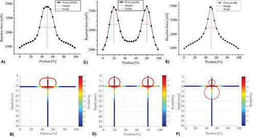
Clinically, PCa is often not focused on a single nodule, therefore the cases of co-existing nodules need to be considered. Figure 7 illustrates three examples. In the cases shown in Figure 7(D), two distinct peaks can be observed given raise by two nodules far apart, whereas the coalesced nodules in Figure 7(B) leads to a force profile which only contains one identifiable peak. When the nodules are dispersed along the depth direction, in Figure 7 (F), the horizontal location is correctly predicted, however the depth has certain under-prediction. This is somewhat expected, since the nodule closer to the surface and the probing could ‘shield’, to a certain degree, the influence of the deeper nodule in the force data. Nevertheless, the proposed method is still capable of predicting the nodules in all three examples, with a good level of accuracy as indicated by the predictive outcomes.

Figure 7. Three representative examples, demonstrating the effects of nodule dispersion along the left-right and anterior-posterior axes on nodule size and location estimation.

4. A clinical feasibility study using ex vivo experimental data

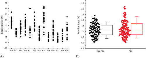
The mechanical data on 13 prostates, previously referred to in Section 2.1, are summarized in Figure 8(A). The forces recorded at the depth of 8 mm ranged between 0 to 3.2 N and each value was associated with a column of tissue directly underneath the probe point, identified as ‘cancerous’ if PCa is identified in that column. Data classified in this way are shown in Figure 8(B) and, as can be seen, it is difficult to distinguish effectively between the cancerous tissue ‘columns’ and the non-cancerous ones using just the raw mechanical data.

Figure 8. Experimental data of probing forces classified by their (A) patient number and (B) the pathological conditions of the ‘tissue column’ directly underneath the probing points (B).

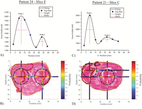
Taking all force profiles along the left-right axis, the proposed methods were used to predict the probability distributions of PCa nodules for each histology section, of which two representative examples are illustrated below. Histology slice E of Patient 24 showed two PCa nodules, outlined in red in Figure 9 (B). Both were identified using the measured force profile shown in Figure 9 (A), and the predicted probabilities of the ‘PCa nodule existence’ were also plotted along both anterior-posterior and left-right axes. Interestingly, although the two force peaks identified have rather different peak values, they have similar values of peak sharpness therefore fall into the same probablistic group (10 < H/W < 20, in Figure 9). In contrast, the histology of slice C of Patient 21 indicated two PCa nodules, very close to each other and the force profile exhibited an extremely sharp peak, resulting in a predicted nodule very close to the posterior surface. The shallower peak resulted in a predicted nodule that was not recognised as PCa by the pathologist (in fact, it is a benign nodule), i.e., a ‘false positive’.

Figure 9. Two example histology slices with associated measured and fitted force profiles, and outlines of prostate and PCa nodules. A probability threshold of 0.5 was used to obtain the predicted PCa nodules (in black).

Classifications based on the predictions of PCa nodules for all patient data are summarized in Table 1, expressed per histological slice and per individual nodule. The classification per histological slice (n = 44) demonstrates the capability of the proposed method, yielding a sensitivity of 92% and specificity of 67%, although the low sample size (n = 6) for condition negative must be acknowledged. For classification at the nodule level (n = 71), 61% of the PCa nodules were correctly identified, which compares very favourably with a recent study of 588 consecutive patients (Johnson et al. 2019), which concluded that “…mpMRI detected 45% of all lesions…”. Furthermore, of those which were not identified, 86% were correctly classified, on a slice basis, through the identification of at least one other PCa nodule on the same slice, giving a sensitivity of 94% (Table 2).

Table 1. Statistical analysis of the prediction, on two classification levels, i.e., histology slices and PCa nodules.

Total histology slices: 44
Condition Positive – PCa in histology: 38 (86%)		Condition Negative – no PCa in histology: 6 (14%)
True Positive 35	False Negative 3	False Positive 2	True Negative 4
Sensitivity 92%		Specificity 67%
Total PCa nodules: 71
Condition Positive – PCa: 71
True Positive 43 (61%)		False Negative 28 (39%)
		At least one other PCa nodule detected in same slice 24 (86%)	No other PCa nodules detected in same slice 4 (14%)

Table 2. Comparison of diagnostic indicators for the current work against dynamic instrumented palpation (Hammer et al. 2019, 2017) and the work of Li et al (Li et al. 2017). Sensitivity (Sens.) = $\mathrm{\%}\left(\frac{TP}{TP+FN}\right),$ Specificity (Spec.) = $\mathrm{\%}\left(\frac{TN}{TN+FP}\right),$ Negative predictive value (NPV) = $\mathrm{\%}\left(\frac{TN}{TN+FN}\right),$ Positive predictive value (PPV) = $\mathrm{\%}\left(\frac{TP}{TP+FP}\right)\mathrm{}$ and Accuracy = $\mathrm{\%}\left(\frac{TP+TN}{TP+FP+FN+TN}\right),$ where “T” and “F” and “P” and “N” have the usual logical meanings (e.g., TP = True positive).

Method	Diagnostic indicator (%)
	Sens.	Spec.	NPV	PPV	Accuracy
Current study: per slice	92	67	57	95	87
Current study: per measurement ‘column’	94	–	–	–	–
Current study: per nodule	61	–	–	–	–
Ex vivo DIP (Hammer et al. 2017)	93	16	59	64	–
In vivo DIP 5 Hz (Hammer et al. 2019)	80	44	64	64	–
RMI (Li et al. 2017)	44	71	56	61	–
DRE (Li et al. 2017)	38	67	52	53	–
MRI (Li et al. 2017)	33	82	55	64	–
TRUS (Li et al. 2017)	76	52	69	62	–

Table 2 puts the results in Table 1 in the context of other mechanical mapping studies of patients at the stage of radical prostatectomy, where the “gold standard” of histological sections is available as base truth. The diagnostic indicators that have been obtained from Table 1 are compared with a recent ex vivo quasi static mechanical mapping study (Li et al. 2017) of 126 sites on 21 patients undergoing robotically minimally invasive radical prostatectomy, and with dynamic mechanical measurements by the authors both ex vivo (Hammer et al. 2017) and in vivo (Hammer et al. 2019). As can be seen, the finding of this study is as sensitive as dynamic ex vivo probing (over 90%) and considerably more sensitive than the rolling mechanical indenter (RMI) (Li et al. 2017). This is irrespective of whether a certain nodule in the slice is detected using the column immediately below the indenter or by identifying other nodules within the same slice. The slightly lower sensitivity of in vivo dynamic probing was attributed to the greater difficulty of placing and orienting the probe, although the sensitivity is still better than reported for TRUS (Li et al. 2017). The specificity of model-informed static probing is considerably better than for dynamic probing and about the same as for the RMI, which is also model-informed. The combination of high sensitivity and specificity means that both NPV and PPV are better than the RMI and very competitive with MRI, DRE and TRUS.

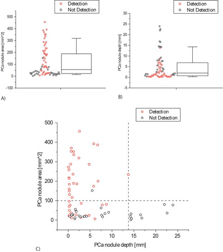
Further to the statistical analysis presented above, and in line with the results obtained from the simplified, simulated models, the classification outcome was affected by the depth and size of the nodules in the histological sections. Of the 60 successfully detected PCa nodules, 42 were located within the first 10 mm below the surface being probed. In addition, 27 of the 45 undetected PCa nodules were smaller than the on-slice area of 100mm², equivalent to a diameter of 11.28 mm. Figure 10 (C) illustrates the ‘depth-size bounds’ in detecting PCa nodules and also shows a region of overlap between the detected and not-detected PCa nodules due to the interplay between the nodule size and depth effects on the force measurements.

Figure 10. Statistical distribution of the tumors volume fraction identified in the histological slices and their distance from the posterior surface.

Table 3 summarizes the prediction result for all 13 prostates, i.e., patients. It should be noted that all patients in this study had at least one PCa nodule and were therefore Condition Positive. On the other hand, the patients were classified by the method as Condition Positive if the force profile exhibited a peak with ratio H/W higher than 5. Once again, the results show the capability of the proposed method to detect PCa nodules close to the posterior surface, with the capability reducing significantly for nodules located more deeply in the prostate.

Table 3. Results of the prediction results for all patients. TP = True positive; FP = False positive; TN = true negative; FN = False negative; det = detected; ud = Un-detected.

Patient No.	Age (y.o.) and Prostate Volume (cc)	Slices	PCa nodule near posterior surface	PCa nodule near anterior surface
P15	60 / 53	3 (TP = 1, FP = 1, TN = 1)	1 (1 det)	1 (1 ud)
P17	60 / 45	3 (TP = 3)	5 (3 det, 2 ud)	1 (1 ud)
P19	58 / 45	4 (TP = 2, TN = 2)	2 (2 det)	0
P20	67 / 86	4 (TP = 2, FP = 1, TN = 1)	3 (2 det, 1 ud)	0
P21	67 / 47	2 (TP = 2)	5 (3 det, 2 ud)	0
P22	64 / 50	4 (TP = 3, FN = 1)	7 (6 det, 1 ud)	0
P23	68 / 51	4 (TP =4)	4 (4 det)	4 (4 ud)
P24	65 / 87	5 (TP = 5)	7 (6 det, 1 ud)	1 (1 ud)
P25	58 / 37	3 (TP = 2, FN = 1)	4 (2 det, 2 ud)	1 (1 ud)
P26	66 / 55	4 (TP = 3, FN = 1)	6 (4 det, 2 ud)	3 (3 ud)
P27	67 / 44	2 (TP = 2)	3 (2 det, 1 ud)	1 (1 ud)
P29	65 / 55	2 (TP = 2)	5 (4 det, 1 ud)	0
P30	68 / 59	4 (TP = 4)	6 (4 det, 2 ud)	1 (1 ud)

5. Conclusions

In this study, a modelling framework was developed to identify and characterize the tumor nodules in prostates using the strategy of point-by-point probing, for which a probabilistic approach has been developed to quantify the uncertainty and enhance the nodule detectability. The approach is based on identifying anomalies (peaks) in the 2-D profiles of point force measurements across transverse “slices” of the prostate and is model-informed. A large number of random cases were generated with various nodule sizes and depths, and probability plots were prepared which relate nodule depth and size to the peak height:width ratio in the 2 D force profile for a given slice. Peaks become more prominent for larger nodules and those closer to the probing surface and it was the non-uniqueness nature of the problem that necessitated such a probability-based approach.

The capability of the proposed method was assessed firstly using a large number of FE models including PCa nodules with randomly generated size, depth and location. The method was capable of characterizing the PCa nodules over a wide range of size and depth, but was less sensitive to those smaller than 5-6mm in diameter.

Force measurement data from 13 ex vivo prostates from patients who had undergone radical prostatatectomy was used to demonstrate the practical application of the method. Promising levels of sensitivity (92%) and specificity (67%) were obtained for ‘diagnosing’ the PCa condition in a total of 44 prostate slices. However, detecting small (diameter < 5 mm) and deep (>14mm, from posterior surface) PCa nodules proved to be more challenging. It is worth pointing out that the detectability may be improved if a greater probing depth, currently 8 mm, is used. The lack of reliable detection for extremely small and deep PCa nodules, albeit not entirely surprising, still signifies a limitation of this study in potential future clinical applications. Nevertheless, this study has shown that model-informed analysis is a useful complementary tool to exisiting methods used for PCa diagnosis, particularly during early screening. Demonstrated through the ex vivo study, its potential to be integrated into the in vivo procedure, such as instrumented DRE (iDRE), will be explored in a future study.

This study, as it currently stands, has a number of limitations. Firstly, all of the patients whose prostates were probed ex vivo had clinically significant cancer, although they had been chosen for the wider study because their disease was largely asymmetric. Thus, there was a relatively small (6 out of 44) number of prostate slices clear of PCa, and no patient had a negative PCa diagnosis. This affects the reliability of the specificity, the PPV and the NPV. Nevertheless, the performance is, overall, better than other published studies in similar groups of patients, and at least as good as MRI, TRUS and conventional DRE. Secondly, the measurements were carried out on excised ex vivo prostates, where the indentation displacement and the location could be controlled much more precisely. Similar probing measurements made in vivo, analogous to the ex vivo measurements reported in this study but transrectally, may be subjected to complications given rise by anatomical features such as the rectal wall. A number of considerations should be given, including various levels of tension in the rectal wall and the bowel pressure, and they will be investigated in a future study. Finally, it was assumed that PCa (and the remainder of the prostate) have a specific quasi-static modulus and that these are the same for every patient. Indeed, due to high variability commonly found in the mechanical behaviors of prostate tissue, this is a simplication and limitation for this study - some cancerous tissue may not be distinguishable from, or could be even softer than, normal counterparts (Lindahl et al. 2021). This may be further complicated by some confounding conditions in prostate, such as benign prostate hyperplasia, however its mechanical properties are believed to be similar to the ‘healthy’ counterpart therefore it would have little influence in the proposed methods for PCa detection. Wider patient studies have shown that there is useful, complementary information in the viscous behaviour of soft tissue for the purpose of cancerous nodule detection (Hammer et al. 2017), and the proposed methods in the context of dynamic tissue behaviors will be exploited in future work. The same wider studies (in hundreds of patients) have also shown that disease-specific changes in stiffness during cancer outweigh patient-specific variation, although this needs to be taken into account in future PCa detection models.

Disclosure statement

No potential conflict of interest was reported by the authors.

Figure A1. Step 1 – Identification of PCa nodule location along the left-right axis.

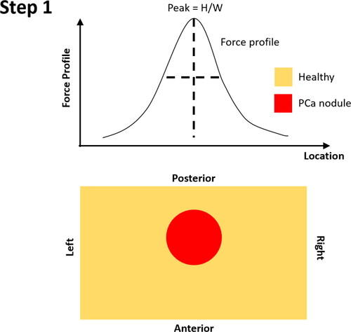
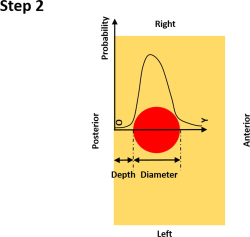
Figure A2. Step 2 – constructing the probability of PCa existence along the anterior-posterior axis, using O as the origin.

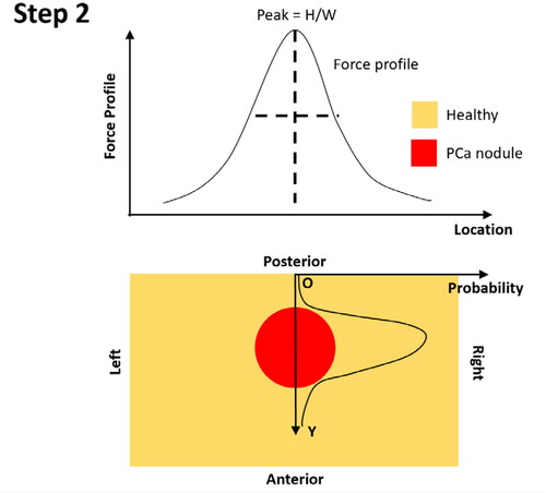
Figure A3. Step 3 – identification of the centre of depth of the PCa nodule.

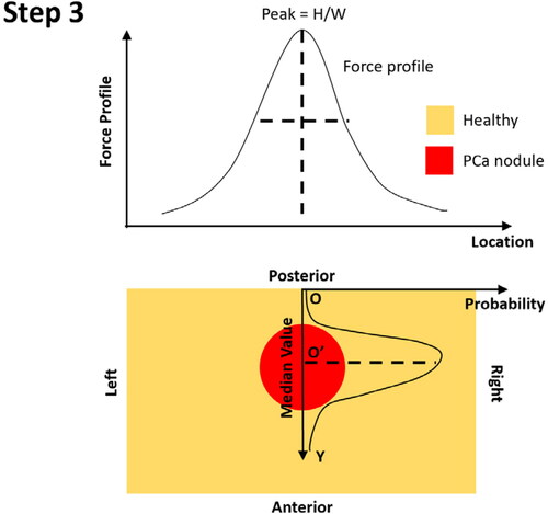
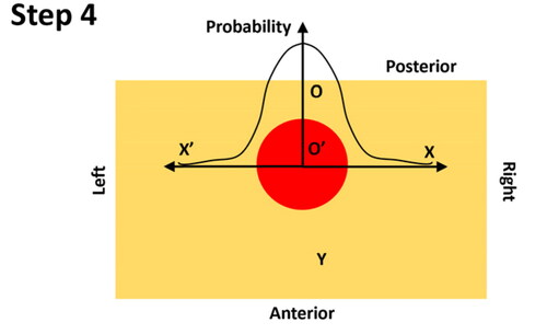
Figure A4. Step 4 – constructing the probability of PCa existence along the left-right axis, using O’ as the origin, in a symmetrical fashion.

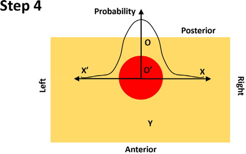
Figure A5. Step 5 –binary identification of PCa nodule using a probability threshold. The effect of the probability threshold is discussed in Electronic Supplementary Material (ESM). In this example the probability threshold was 0.5.

Additional information

Funding

The authors gratefully acknowledge support from the Engineering and Physical Sciences Research Council (EPSRC) under grants nos. EP/I019472/1, EP/I020101/1 and EP/N006089/1. This study was also supported by the James Watt PhD scholarship awarded to the first author. The support from the Department of Pathology at the Western General Hospital is greated appreciated.

Appendix A. Identification of PCa nodules in prostate

This section is designed to demonstrate the process of identifying the PCa nodules in prostate based on the force profile from probing its posterior surface.

• Step 0: Identify the peak in the force profile – the value of sharpness, H/W, needs to be greater than 5; Peaks with H/W value lower than 5 are believed to be un-identifiable.

• Step 1: Identify the location of the peak of force profile along the left-right axis, which is considered to be the ‘horizontal’ location of the identified PCa nodule;

• Step 2: Once the location of the PCa nodule is identified, the probability of nodule existence is calculated, firstly, along the anterior-posterior axis, using the identified location at the posterior surface as the ‘origin’. It should be noted that the probability along the anterior-posterior direction depends on both the PDFs of the nodule depth and size (see Appendix B).

• Step 3: Along the anterior-posterior axis, the centre of the PCa nodule is identified using the median value of the probability distribution along the Y-axis.

• Step 4: At the depth of the identified tumor centre, the probability of the nodule existence along the left-right axis is calculated, in a symmetric fashion, using the O’ as the origin. Note the probability along the left-right axis only depends on the PDF of the nodule size (see Appendix B).

• Step 5: if binary prediction, i.e. the outline of the PCa nodule, is needed, a probability threshold, as illustrated as a ‘virtual plane’, can be adopted and the area along two major axes with probability values greater than the chosen threshold is believed to be the area of PCa nodule (i.e. the circle projected onto the depth-position plane).

Appendix B.

Predicting probabilities along left-right and anterior-posterior axes

This section describes how the probabilities of the PCa nodule existence along both the left-right and anterior-posterior axes are derived. The probability is defined to be the likelihood of a given point in the prostate domain being a part of the PCa nodule. The following derivation follows a 1 D simplification, using the coordinate systems defined in Appendix A, for both axes, respectively.

Figure B1. Schematic of the equivalent 1 D problem for finding the probability along the Y axis.

B.1. Probability along the anterior-posterior axis (step 2 in Appendix A)

Let the nodule depth ($d$) and diameter ($D$) be two independent random variables, which can take non-negative real numbers. Mathematically, the probability of any given non-negative real number a (i.e., any given location on the $Y$ axis, a constant, rather than a random variable) being no less than d and no greater than $d+D$ or $Z$ can be expressed as (B1) $$d\le a\le d+D\mathrm{}or\mathrm{}Z$$(B1)

Physically, this means the location of any given point falling in the red region along the Y axis. The probability density functions (PDFs) of the nodule depth ($d$ and its PDF $f$) and diameters ($D$ and its PDF $g$) are presented in Fig. 4.

The random variable $Z,$ i.e., d + D, has its PDF $h.$ We can derive h, using the rule of convolution, with both f and g. (B2) $$h=\mathrm{}{\int }_{-\mathrm{\infty }}^{+\mathrm{\infty }}f\left(z-D\right)g\left(D\right)dD$$(B2)

Therefore, the joint probability can be calculated as (B3) $$\mathrm{Pr}\left(d\le a\le Z\right)=\mathrm{Pr}\left(d\le a\right)-\mathrm{Pr}(d\le a\mathrm{}\mathit{and}\mathrm{}Z\le a)$$(B3)

Note $\mathrm{Pr}\left(d\le a\right)={\int }_0^{a}f.$ Therefore, we need to get $\mathrm{Pr}(d\le a\mathrm{}\mathit{and}\mathrm{}Z\le a).$ Such a joint probability between d and $Z$ can be calculated by the convention of joint probability, i.e., multiplying the conditional distribution of d$\le a$ given Z$\le a,$ with marginal distribution of Z$\le a.$

Figure B2. Step 4 – deriving the probability along the left-right axis.

It is later proved [see Proof 1 below] that the joint probability of $\mathrm{Pr}(d\le a\mathrm{}\mathit{and}\mathrm{}Z\le a)$ takes, coincidentally due to the formulation of the $Z,$ the same form as $\mathrm{Pr}(Z\le a).$ Therefore, (B4) $$\mathrm{Pr}\left(d\le a\le X+Y\right)=\mathrm{Pr}\left(d\le a\right)-\mathrm{Pr}\left(Z\le a\right)={\int }_0^{a}f-{\int }_0^{a}h$$(B4)

[Proof 1] The joint probability, which is the $\mathrm{Pr}(d\le a\mathit{and}Z\le a)$ as put earlier, is equal to the conditional distribution of d$\le a$ given $Z\le a$ multiplied by marginal distribution of $Z\le a$. Note that the marginal distribution of Z, i.e. when $Z\le a$, is equal to $\mathrm{Pr}\left(Z\le a\right)={\int }_0^{a}h$. On the other hand, the conditional distribution of $d\le a$ given $Z\le a$, in other words, the probability of $d\le a$ when $d+D\le a$, is always 1, since D must take non-negative value. Therefore, the joint probability between X and Z is the same as that of Z.

B.2. Probability along the left-right axis (step 4 in Appendix A)

It is evident that the probability along the left-right axis (X and X’ axes as shown in Fig. B2) is only dependent on the random variable D, i.e., the diameter of the PCa nodule. Using the same approach in B.1, the probability of any given non-negative real number b (i.e., any given location along the X or X’ axes, which is a constant, not a random variable) being no greater than D/2 (i.e., radius of PCa nodule). (B5) $$b\le D/2$$(B5)

Assuming the PDF of D/2 takes the form of q, which can be derived conveniently from the PDF of D, i.e., g(D), the probability along left-right axis can be expressed as (B6) $$\mathrm{Pr}\left(b\le \frac{D}{2}\right)={\int }_b^{\mathrm{\infty }}q$$(B6)

References

- Ahn B, Kim J. 2009. Efficient soft tissue characterization under large deformations in medical simulations. Int J Precis Eng Manuf. 10(4):115–121.
- Baghban M, Mojra A. 2018. Early relaxation time assessment for characterization of breast tissue and diagnosis of breast tumors. J Mech Behav Biomed Mater. 87:325–335.
- Carson WC, Gerling GJ, Krupski TL, Kowalik CG, Harper JC, Moskaluk C a. 2011. Material characterization of ex vivo prostate tissue via spherical indentation in the clinic. Med Eng Phys. 33(3):302–309.
- Cox M, Driessen N, Boerboom RA, Bouten C, Baaijens F. 2008. Mechanical characterization of anisotropic planar biological soft tissues using finite indentation: Experimental feasibility. J Biomech. 41(2):422–429.
- Hammer SJ, Good DW, Scanlan P, Palacio-Torralba J, Phipps S, Stewart GD, Shu W, Chen Y, McNeill SA, Reuben RL. 2017. Quantitative mechanical assessment of the whole prostate gland ex vivo using dynamic instrumented palpation. Proc Inst Mech Eng H. 231(12):1081–1100.
- Hammer SJ, Johnson O, Good DW, Palacio-Torralba J, Candito A, Chen Y, Phipps S, Shu W, McNeill SA, Reuben RL. 2019. Mechanical mapping of the prostate in vivo using Dynamic Instrumented Palpation; towards an in vivo strategy for cancer assessment. Proc Inst Mech Eng Part H, J Eng Med. Under review.
- Hosseini SM, Amiri M, Najarian S, Dargahi J. 2007. Application of artificial neural networks for the estimation of tumour characteristics in biological tissues. Int J Med Robot. 3(3):235–244.
- Hoyt K, Castaneda B, Zhang M, Nigwekar P, di Sant'Agnese PA, Joseph JV, Strang J, Rubens DJ, Parker KJ. 2008. Tissue elasticity properties as biomarkers for prostate cancer. CBM. 4(4–5):213–225.
- Johnson DC, Raman SS, Mirak SA, Kwan L, Bajgiran AM, Hsu W, Maehara CK, Ahuja P, Faiena I, Pooli A, et al. 2019. Detection of individual prostate cancer foci via multiparametric magnetic resonance imaging. Eur Urol. 75(5):712–720.
- Keshavarz M, Mojra A. 2015. Geometrical features assessment of liver’s tumor with application of artificial neural network evolved by imperialist competitive algorithm. Int J Numer Method Biomed Eng. 2015 May;31(5):e02704. doi: 10.1002/cnm.2704.
- Kim Y, Ahn B, Na Y, Shin T, Rha K, Kim J. 2014. Digital rectal examination in a simulated environment using sweeping palpation and mechanical localization. Int J Precis Eng Manuf. 15(1):169–175.
- Krouskop TA, Wheeler TM, Kallel F, Garra BS, Hall T. 1998. Elastic moduli of breast and prostate tissues under compression. Ultrason Imaging. 20(4):260–274.
- Li J, Liu H, Brown M, Kumar P, Challacombe BJ, Chandra A, Rottenberg G, Seneviratne LD, Althoefer K, Dasgupta P. 2017. Ex vivo study of prostate cancer localization using rolling mechanical imaging towards minimally invasive surgery. Med Eng Phys. 43:112–117.
- Lindahl OA, Backlund T, Ramser K, Liv P, Ljungberg B, Bergh A. 2021. A tactile resonance sensor for prostate cancer detection – evaluation on human prostate tissue. Biomed Phys Eng Express. 7(2):025017.
- Liu H, Sangpradit K, Li M, Dasgupta P, Althoefer K, Seneviratne LD. 2014. Inverse finite-element modeling for tissue parameter identification using a rolling indentation probe. Med Biol Eng Comput. 52(1):17–28.
- Miller K. 2005. Method of testing very soft biological tissues in compression. J Biomech. 38(1):153–158.
- Nichols KA, Okamura AM. 2015. Methods to segment hard inclusions in soft tissue during autonomous robotic palpation. IEEE Trans Robot. 31(2):344–354.
- Palacio-Torralba J, Hammer S, Good DW, Alan McNeill S, Stewart GD, Reuben RL, Chen Y. 2015. Quantitative diagnostics of soft tissue through viscoelastic characterization using time-based instrumented palpation. J Mech Behav Biomed Mater. 41:149–160.
- Palacio-Torralba J, Jiménez Aguilar E, Good DW, Hammer S, Mcneill SA, Stewart GD, Reuben RL, Chen Y. 2016. Patient specific modeling of palpation-based prostate cancer diagnosis: Effects of pelvic cavity anatomy and intrabladder pressure. Int J Numer Method Biomed Eng. 32:1–13.
- Phipps S, Yang T, Habib FK, Reuben RL, McNeill SA. 2005. Measurement of the mechanical characteristics of benign prostatic tissue: A Novel method for assessing benign prostatic disease. Urology. 65(5):1024–1028.
- Sangpradit K, Liu H, Dasgupta P, Althoefer K, Seneviratne LD. 2011. Finite-element modeling of soft tissue rolling indentation. IEEE Trans Biomed Eng. 58(12):3319–3327.
- Scanlan P, Hammer SJ, Good DW, Phipps S, Stewart GD, McNeill SA, Shu W, Reuben RL. 2015. Development of a novel actuator for the dynamic palpation of soft tissue for use in the assessment of prostate tissue quality. Sensors Actuators, A Phys. 232:310–318.
- Torlakovic G, Grover VK, Torlakovic E. 2005. Easy method of assessing volume of prostate adenocarcinoma from estimated tumor area: Using prostate tissue density to bridge gap between percentage involvement and tumor volume. Croat Med J. 46(3):423–428.
- Yang Y, Guo S, Hao Z. 2018. Correlation between stress drop and applied strain as a biomarker for tumor detection. J Mech Behav Biomed Mater. 86:450–462.