Characterisation of the climatic temperature variations in the design of rigid pavements

ABSTRACT

The design of rigid pavements in Austria is currently based on a catalogue of standard structures, which can be chosen depending on traffic-related parameters. This approach does not allow the consideration of real material characteristics, detailed traffic load information, local climate conditions, and other boundary conditions. To overcome these limitations, a new mechanistic-empirical pavement design method for rigid pavements (MEPDR) has been developed. The focus of this paper is laid on the proper characterisation of climatic boundary conditions and their impact on the design results. To simulate the actual temperature distribution within a concrete slab, a temperature prediction model was proposed and validated with measured weather data. Furthermore, representative temperature gradients were established using the proposed model and surface temperature data from measuring stations distributed over the Austrian highway pavement network. Additionally, the effect of these temperature gradients on the design life of a typical pavement structure was demonstrated using the MEPDR.

KEYWORDS:

• Design of rigid pavements
• temperature distribution
• curling stresses
• design life

1. Introduction

The old Austrian design method for rigid pavements RVS 03.08.63 (FSV 2016) defines standard pavement structures for different load classes in a design catalogue. The method is based on semi-analytical models, using physical and mechanical principles to describe the reaction of a rigid pavement to external loads. However, this method has some limitations regarding the consideration of real material characteristics, detailed load information and various climatic boundary conditions. The drawbacks of the design process lead to ticker and less economic pavement structures. To resolve these limitations, a new mechanistic-empirical pavement design method for rigid pavements (MEPDR) has been developed in Austria (Eberhardsteiner et al. 2016, 2018; FSV 2020). The new Austrian MEPDR method considers several input parameters and allows for the prediction of service life or estimation of allowable load cycles until failure. Moreover, the design method offers more realistic modelling of traffic loads by incorporating actual data of traffic volume, vehicle gross weight and axle load distribution, so that traffic loads can be taken into account as realistic as possible. It also considers the load transfer in transverse joints by using a dowel effectiveness number (DEN) and the actual concrete material behaviour by using experimental results of tensile bending tests or splitting tensile tests. Another important factors affecting the pavement performance are the climatic boundary conditions. The subgrade bearing capacity is strongly influenced by local climatic and hydrological conditions. Hence, four periods during one year with varying subgrade modulus representative for bearing capacities of soils are considered in Austria. Additionally, the temperature distribution within the concrete slab (temperature difference between the top and the bottom of the slab) can force the slab to warp upward or downward, which will affect the pavement's performance under traffic load. Therefore, the fatigue behaviour of concrete is described by Smith's criterion (Eisenmann 1979), which takes into account traffic and curling stresses.

To establish representative temperature gradients for the estimation of curling stresses and to account for seasonal and local temperature variations in the pavement design, the temperature distribution in rigid pavements has been investigated using actual weather data (Eberhardsteiner et al. 2016; Bayraktarova et al. 2017). Therefore, a temperature prediction model based on the Forward Time Centered Space (FTCS) Finite Difference Method (FDM) was implemented in a tool and validated using actual temperature measurements. Furthermore, the impact of the temperature gradients on the design life of rigid pavements was demonstrated using the Austrian MEPDR (FSV 2020).

2. Literature review

The investigation of temperature and moisture variations in rigid pavement structures is an important task, as these fluctuations generate volumetric changes of the concrete slabs and induce curling or warping stresses. Consequently, these stresses cause upward or downward slab curvature, which, in combination with the traffic loading, can lead to fatigue damage. To create a proper perspective, the following section reviews state of the art models for the prediction of temperature profiles in pavements as well as different approaches for the calculation of curling stresses in rigid pavements.

2.1. Prediction of temperature profiles

As temperature variations play a crucial role in the development of critical stress and distress, temperature distribution in a pavement is considered in most Mechanistic Empirical Pavement Design Models (NCHRP 2004). Wang et al. (2009) summarised three types of solution methods to predict pavement temperature profiles: statistics-based, analytical and numerical approaches. A comprehensive review of existing models for predicting pavement temperature, including empirical, analytical, and numerical models is given in Chen et al. (2019).

Statistics-based methods use simplified correlations between pavement temperature and environmental factors. These methods can be categorised in linear regression models, nonlinear regression models, and neural network models. The linear regression models calculate extreme or average temperature in pavement at a prescribed depth within an original sample database and should not be extrapolated outside the original solution database (Sherif and Hassan 2004; Diefenderfer et al. 2002; Krsmanc et al. 2013). The nonlinear regression models are more complex and allow the prediction of pavement temperature with time and depth (Chandrappa and Biligiri 2015). The prediction of pavement temperature with neural network models is based on machine learning using extensive data.

Analytical and numerical models can be formulated by solving the partial differential equation (PDE) for heat conduction under given boundary conditions to simulate time-dependent temperature profiles. These methods use pavement geometry, climatic and thermal parameters of the layered materials.

Barber (1957) was among the first researchers to employ an analytical solution to the heat conduction problem for prediction of pavement temperatures. In his solution, a thermal diffusion theory was applied to a semi-infinite pavement in contact with air temperature. However, the model operates with total daily radiation instead of hourly radiation and is therefore inaccurate.

Dempsey and Thompson (1970) developed an approach that uses 1D heat transfer model and an explicit finite difference method (FDM) to simulate temperature profiles as a function of time. His approach was implemented in the Mechanistic Empirical Pavement Design Guide (MEPDG) (NCHRP 2004) as part of the Enhanced Integrated Climatic Model (EICM). EICM considers hourly climatic data that include air temperature, wind speed, relative humidity, precipitation, percentage of sunshine and location of ground water to calculate the temperature and moisture profile, frost heave and other climate-related phenomena.

Later, Solaimanian and Kennedy (1993) considered energy balance at the pavement surface and developed an equation for calculating the maximum pavement surface temperature. Wang proposed analytical models developed by solving the PDE for heat conduction using the separation of variables method (Wang 2012; Wang and Roesler 2014) and eigenfunction expansion technique (Wang 2016). Qin (2016) introduced a prediction model for pavement surface temperature based on the assumption that the daily surface temperature follows sinusoidal waves.

Many researches (Hermansson 2002; Yavuzturk et al. 2005; Huang et al. 2017) developed numerical models with FDM for prediction of temperature profiles, that use solar radiation, long-wave radiation and convection to define the surface boundary condition.

Besides FDM, the Finite Volume Method (FVM) and the Finite Element Method (FEM) can also be applied to predict the pavement temperature. These models are appropriate for complex surface boundary conditions because the PDE of heat conduction is solved over the nodes or volumes numerically. In the literature, there are plenty of FEM-models for predicting temperature profiles (McCullough and Rasmussen 1999; Minhoto et al. 2005; Jeong and Zollinger 2006; Teltayev and Koblanbek 2015). Alavi et al. (2014) proposed a temperature prediction model using the finite control volume approach (FCVM) with fully implicit scheme, that solved some of the known limitations in current temperature prediction models.

2.2. Calculation of the curling stresses in rigid pavements

The most common way to consider temperature distribution in the estimation of curling stresses is to use linear temperature gradients $\mathrm{\Delta }T$, even though the nonlinearity of the temperature distribution throughout the slab has long been recognised (Choubane and Tia 1995; Mohamed and Hansen 1996; Siddique et al. 2005). A temperature gradient arises from the temperature difference on the top and on the bottom of the concrete slab divided by its thickness.

The Eisenmann 's and Westergaard–Bradbury‘s approximate analytical solutions are the most commonly used and are based on Kirchhoff's plate theory. They are based, for simplicity, on the assumption that the temperature variation in the concrete slab from top to bottom is linear.

Bradbury (1938) solution assumes linear temperature differential, Winkler foundation and full bonding between the slab and the foundation. The curling stress can be estimated for any pavement structure by taking into account the effective thickness of the slab with the corresponding radius of relative stiffness values.

Eisenmann's solution (Eisenmann 1979) is based on the concept of a critical slab length $L_{\mathrm{c}\mathrm{r}\mathrm{i}\mathrm{t}}$, which is defined as the length where a concrete slab, equally heated at the surface, only touches the substructure at the four corners and in its centre. Three cases are considered depending on the actual length of the slab L. When $L>1.1\cdot L_{\mathrm{c}\mathrm{r}\mathrm{i}\mathrm{t}}$, the stress in the centre of the slab can be determined according to Kirchhoff's plate theory. When $L\approx L_{\mathrm{c}\mathrm{r}\mathrm{i}\mathrm{t}}$ the stress increases by 20% and when $L<0.9\cdot L_{\mathrm{c}\mathrm{r}\mathrm{i}\mathrm{t}}$, the stress reduces depending on the actual length of the slab L. In the early nineties, it was found that the Eisenmann's model for calculation of the curling stresses is not accurate for estimation of the critical stresses resulting from great temperature gradients. Houben (1992) revised Eisenmann's model and introduced a coefficient C for the support length for different temperature gradients.

While the Bradbury (1938) solution assumes full bonding between the slab and the foundation, Eisenmann's solution (Eisenmann 1979) considers partial foundation contact, which corresponds to the real interface behaviour.

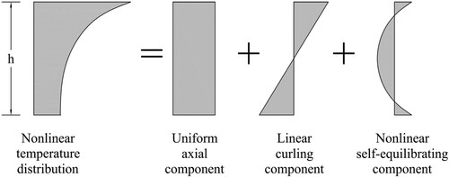
Thomlinson (1940) was the first researcher who developed a theory, accounting for the nonlinear temperature distribution in the estimation of curling stresses. According to him, the total curling stress can be divided into three components (Figure 1). The first uniform axial component causes the slab to expand or contract. The second is the linear component due to temperature changes that causes bending (upward or downward) and the third is the nonlinear component, which generates internal forces as a result from the temperature loading and the restriction of the deformations.

Figure 1. Components of the nonlinear temperature-induced deformation (Thomlinson 1940; Eisenmann 1979).

Another concept to estimate a temperature gradient is to convert the nonlinear temperature profile to an equivalent temperature difference $\mathrm{\Delta }{T}_{\mathrm{e}\mathrm{q}}$ (Thomlinson 1940; Choubane and Tia 1995; Mohamed and Hansen 1996; Ioannides and Khazanovich 1998). This equivalent temperature difference would induce the same slab curvature as the original nonlinear temperature profile. Ioannides and Khazanovich (1998) established this concept of a non-uniform, multi-layered slab and implemented it into finite-element code ILSL2 and MEPDG (NCHRP 2004). The estimation of critical stresses in the MEPDG is based on Neural Networks matching prediction from the finite element model ISLAB2000. This model is a generalisation of the Westergaard solution and considers a variety of design factors (Khazanovich et al. 2001): surface and base layer parameters, interface conditions between the concrete slab and the base layer, shoulder type, slab geometry, subgrade properties, axle type, weight, and position and the effect of voids under pavements. The MEPDG also considers the effect of the built-in temperature gradient or construction temperature gradient. Eisenmann and Leykauf (1990) found out that constructing concrete pavements in hot days induces a large positive temperature gradient during the hardening, that is the cause for early upward curling. Yu et al. (1998) studied the effects of the built-in temperature curling on the critical wheel load stress. Beckemeyer et al. (2002) demonstrated the influence of the base layer type on the magnitude of built-in curling. Later Rao and Roesler (2005) introduced the effective built-in temperature difference, combining the effects of temperature, shrinkage, and creep.

Hiller and Roesler (2010) proposed a nonlinear area method called NOLA that captures the effect of temperature nonlinearity. Lately, a strain-based equivalent temperature gradient $\mathrm{\Delta }{T}_{\mathrm{s}\mathrm{t}\mathrm{r}\mathrm{a}\mathrm{i}\mathrm{n}}$ was proposed by Gao et al. (2017). They found that $\mathrm{\Delta }{T}_{\mathrm{s}\mathrm{t}\mathrm{r}\mathrm{a}\mathrm{i}\mathrm{n}}$ is the smallest among $\mathrm{\Delta }T$ and $\mathrm{\Delta }{T}_{\mathrm{e}\mathrm{q}}$, because of the added effect of moisture gradient which causes upward warping equivalent to a negative temperature gradient. It was recommended to use $\mathrm{\Delta }T$ for design purposes because of the conservative, calculated curling that a linear temperature gradient provides.

The curling stresses can also be calculated using a numerical method, although they are time-consuming, costly and require an understanding of the complexity of the problem.

Furthermore, comparative studies (Eberhardsteiner et al. 2016; Caliendo and Parisi 2010) of the calculated curling stresses with Westergaard–Bradbury's model, Eisenman's model and a 3D FE model (ABAQUS/Standard 2014) have shown a good agreement between the Eisenmann's and the FE solutions at the slab edge (Table 1). In consequence of these results and for simplicity, the revised Eisenmann–Houben model was implemented in the new Austrian mechanistic pavement design method for rigid pavements.

Table 1. Maximum tensile stresses according to different models (Eberhardsteiner et al. 2016).

	Maximum tensile stresses according to different models (N/mm${}^2$)
Location	Bradbury	Eisenmann	Eisenmann–Houben	FE-Abaqus
Slab edge	3.45	1.31	1.34	1.47
Percentage difference	157%	−2%	–	10%

3. Simulation of temperature distribution

As aforementioned, the FDM can be employed to solve the differential equation and predict pavement temperature distribution. The following section presents a numerical solution of the Fourier heat equation with a Finite Difference Method and describes the input parameters and demonstrates that the model is capable of reproducing measured temperature data.

3.1. Finite difference method (FDM)

The Fourier equation (1(1) $\frac{\mathrm{\partial }T}{\mathrm{\partial }t}=\alpha \cdot \frac{{\mathrm{\partial }}^{2}T}{\mathrm{\partial }{x}^2}$(1) ) for the one-dimensional case describes a transient heat transfer or the change in temperature T [K], in a solid environment, without any internal heat source as a function of time t [s] and depth x (location coordinate) [m]. (1) $\frac{\mathrm{\partial }T}{\mathrm{\partial }t}=\alpha \cdot \frac{{\mathrm{\partial }}^{2}T}{\mathrm{\partial }{x}^2}$(1) Where the thermal diffusivity α describes the rate of thermal energy spreading through the material. By this means, the thermal diffusivity can be calculated as a quotient of thermal conductivity and heat capacity. The thermal conductivity λ [$\mathrm{W}\cdot {\mathrm{m}}^{-1}\cdot {\mathrm{K}}^{-1}$] describes the ability of a stratum with density ρ [$\mathrm{k}\mathrm{g}\cdot {\mathrm{m}}^{-3}$] to conduct and the specific heat capacity c [$\mathrm{J}\cdot {\mathrm{k}\mathrm{g}}^{-1}\cdot {\mathrm{K}}^{-1}$] describes the ability to store thermal energy. (2) $\alpha =\frac{\lambda }{c\cdot \rho }$(2) For numerical evaluation, the exact solution is approximated by finite time intervals $\mathrm{\Delta }t$ and thickness intervals $\mathrm{\Delta }x$. Hereby, the temperature change $\mathrm{\Delta }{T}_t$ occurring during the time interval $\mathrm{\Delta }t$ can be written as (3) $\mathrm{\Delta }{T}_t=\alpha \cdot \frac{\mathrm{\Delta }t}{\mathrm{\Delta }{x}^2}\cdot {\mathrm{\Delta }}^2{T}_x$(3) where $\mathrm{\Delta }{T}_t$ describes the change of temperature by time, $\mathrm{\Delta }{T}_x$ the change by position and ${\mathrm{\Delta }}^2{T}_x$ the difference between two successive differences. Now, the indices k for the time step and n for the position step are introduced, as is shown in Figure 2.

Figure 2. Index scheme for numerical evaluation, where the horizontal shift describes the change of temperature by time and the vertical shift the change of temperature by position.

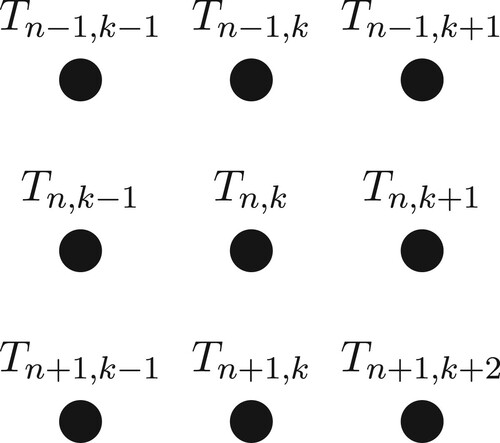
With this in mind, the differences between two nodes can be written as (4) $\mathrm{\Delta }{T}_t=T_{n,k+1}-T_{n,k}$(4) (5) $\mathrm{\Delta }{T}_x=T_{n+1,l}-T_{n,k}$(5) (6) $\begin{array}{rl}{\mathrm{\Delta }}^2{T}_x& =(T_{n+1,k}-T_{n,k})-(T_{n,k}-T_{n-1,k})\\ & =T_{n+1,k}-2\cdot T_{n,k}+T_{n-1,k}\end{array}$(6) Inserting Equations (4(4) $\mathrm{\Delta }{T}_t=T_{n,k+1}-T_{n,k}$(4) ) and (6(6) $\begin{array}{rl}{\mathrm{\Delta }}^2{T}_x& =(T_{n+1,k}-T_{n,k})-(T_{n,k}-T_{n-1,k})\\ & =T_{n+1,k}-2\cdot T_{n,k}+T_{n-1,k}\end{array}$(6) ) in Equation (3(3) $\mathrm{\Delta }{T}_t=\alpha \cdot \frac{\mathrm{\Delta }t}{\mathrm{\Delta }{x}^2}\cdot {\mathrm{\Delta }}^2{T}_x$(3) ) leads to the explicit FTCS (Forward Time Centered Space) FDM in Equation (7(7) $T_{n,k+1}=\alpha \cdot \frac{\mathrm{\Delta }t}{\mathrm{\Delta }{x}^2}\cdot (T_{n+1,k}-2\cdot T_{n,k}+T_{n-1,k})+T_{n,k}$(7) ). (7) $T_{n,k+1}=\alpha \cdot \frac{\mathrm{\Delta }t}{\mathrm{\Delta }{x}^2}\cdot (T_{n+1,k}-2\cdot T_{n,k}+T_{n-1,k})+T_{n,k}$(7) The explicit FTCS scheme provides, as in Krebs and Böinger (1981) and Dempsey et al. (1985) shown, reliable and straightforward results. The scheme is numerically stable when Equation (8(8) $\alpha \cdot \frac{\mathrm{\Delta }t}{\mathrm{\Delta }{x}^2}\le \frac{1}{2}$(8) ) is satisfied. (8) $\alpha \cdot \frac{\mathrm{\Delta }t}{\mathrm{\Delta }{x}^2}\le \frac{1}{2}$(8) The explicit scheme needs to be adapted in order to solve the equation with a mixed condition, where the surrounding temperature is given while the surface temperature is unknown. Under the assumption that the heat flow only depends on the heat transfer between the surrounding air and the surface of the body, the heat balance equation can be written as (9) $\lambda \cdot \frac{\mathrm{d}T}{\mathrm{d}x}=h\cdot (T_A-T_S).$(9) Where the left-hand side term represents the heat conduction and the right-hand side, the heat transfer between the air and the surface. The heat transfer describes the amount of heat exchanged per area and time between the air and the ground surface and is formulated as a function of the heat transfer coefficient h [$\mathrm{W}\cdot {\mathrm{m}}^{-2}\cdot {\mathrm{K}}^{-1}$]. It can be represented as a function of the wind speed u [$\mathrm{m}\cdot {\mathrm{s}}^{-1}$]. Krebs and Böinger (1981) have derived an empirical formulation (11(11) $h\left(t\right)=10\cdot (0.174+0.941\cdot u(t{)}^{0.366})$(11) ) from measurements on the surface. (10) $h\left(t\right)=c_1+c_2\cdot u(t{)}^{c_3}$(10) (11) $h\left(t\right)=10\cdot (0.174+0.941\cdot u(t{)}^{0.366})$(11) Where $u\left(t\right)\left[\mathrm{m}\cdot {\mathrm{s}}^{-1}\right]$ represents the wind speed in 10 m height and $c_1,c_2$ and $c_3$ are empirically determined constants. Now the temperatures at position n = 1 can be written as (12) $T_{1,k+1}=\alpha \cdot \frac{\mathrm{\Delta }t}{\mathrm{\Delta }{x}^2}\cdot \left[T_{2,k}-2\cdot T_{1,k}-\frac{T_{A,k}-T_{S,k}}{\frac{\lambda }{h_k}}\cdot \left(\frac{\lambda }{h_k}-\frac{\mathrm{\Delta }x}{2}\right)+T_{A,k}\right]+T_{1,k}$(12) and the temperatures at the surface n = 0 as (13) $T_{S,k+1}=-\frac{T_{A,k+1}-T_{1,k+1}}{\left(\frac{\lambda }{h_{k+1}}+\frac{\mathrm{\Delta }x}{2}\right)}\cdot \frac{\lambda }{h_{k+1}}+T_{L,k+1}.$(13) For the temperatures at positions $n>1,$ the application remains unchanged using Equation (7(7) $T_{n,k+1}=\alpha \cdot \frac{\mathrm{\Delta }t}{\mathrm{\Delta }{x}^2}\cdot (T_{n+1,k}-2\cdot T_{n,k}+T_{n-1,k})+T_{n,k}$(7) ). To describe the influence of the radiation balance, the reduced heat balance Equation (9(9) $\lambda \cdot \frac{\mathrm{d}T}{\mathrm{d}x}=h\cdot (T_A-T_S).$(9) ) needs to be supplemented by the solar radiation Q $\left[\mathrm{K}\cdot {\mathrm{m}}^{-2}\right]$. (14) $\lambda \cdot \frac{\mathrm{d}T}{\mathrm{d}x}=h\cdot (T_A-T_S)+Q$(14) For an unchanged application of the scheme, Krebs and Böinger (1981) introduced a virtual air temperature $T_A^{\ast }$, where all energy flows on the surface are subsumed. (15) $h\cdot (T_A^{\ast }-T_S)=h\cdot (T_A-T_S)+Q$(15) (16) $T_A^{\ast }=T_A+\frac{Q}{h}$(16) Inserting Equation (16(16) $T_A^{\ast }=T_A+\frac{Q}{h}$(16) ) in Equations (13(13) $T_{S,k+1}=-\frac{T_{A,k+1}-T_{1,k+1}}{\left(\frac{\lambda }{h_{k+1}}+\frac{\mathrm{\Delta }x}{2}\right)}\cdot \frac{\lambda }{h_{k+1}}+T_{L,k+1}.$(13) ) and (12(12) $T_{1,k+1}=\alpha \cdot \frac{\mathrm{\Delta }t}{\mathrm{\Delta }{x}^2}\cdot \left[T_{2,k}-2\cdot T_{1,k}-\frac{T_{A,k}-T_{S,k}}{\frac{\lambda }{h_k}}\cdot \left(\frac{\lambda }{h_k}-\frac{\mathrm{\Delta }x}{2}\right)+T_{A,k}\right]+T_{1,k}$(12) ) leads to Equations (17(17) $T_{S,k+1}=-\frac{T_{A,k+1}^{\ast }-T_{1,k+1}}{\left(\frac{\lambda }{h_{k+1}}+\frac{\mathrm{\Delta }x}{2}\right)}\cdot \frac{\lambda }{h_{k+1}}+T_{A,k+1}^{\ast }$(17) ) and (18(18) $T_{1,k+1}=a\cdot \frac{\mathrm{\Delta }t}{\mathrm{\Delta }{x}^2}\cdot \left[T_{2,k}-2\cdot T_{1,k}-\frac{T_{A,k}^{\ast }-T_{S,k}}{\frac{\lambda }{h_k}}\cdot \left(\frac{\lambda }{h_k}-\frac{\mathrm{\Delta }x}{2}\right)+T_{A,k}^{\ast }\right]+T_{1,k}$(18) ). Together with Equation (7(7) $T_{n,k+1}=\alpha \cdot \frac{\mathrm{\Delta }t}{\mathrm{\Delta }{x}^2}\cdot (T_{n+1,k}-2\cdot T_{n,k}+T_{n-1,k})+T_{n,k}$(7) ) all equations to calculate the temperature profile with mixed boundary conditions are presented. The dependencies are shown in Figure 3 and the algorithm is presented in Figure 4. (17) $T_{S,k+1}=-\frac{T_{A,k+1}^{\ast }-T_{1,k+1}}{\left(\frac{\lambda }{h_{k+1}}+\frac{\mathrm{\Delta }x}{2}\right)}\cdot \frac{\lambda }{h_{k+1}}+T_{A,k+1}^{\ast }$(17) (18) $T_{1,k+1}=a\cdot \frac{\mathrm{\Delta }t}{\mathrm{\Delta }{x}^2}\cdot \left[T_{2,k}-2\cdot T_{1,k}-\frac{T_{A,k}^{\ast }-T_{S,k}}{\frac{\lambda }{h_k}}\cdot \left(\frac{\lambda }{h_k}-\frac{\mathrm{\Delta }x}{2}\right)+T_{A,k}^{\ast }\right]+T_{1,k}$(18) The radiation balance is given by (19) $Q=Q_{ns}+Q_{nl}$(19) where $Q_{ns}$ $\left[\mathrm{W}\cdot {\mathrm{m}}^{-2}\right]$ is the net short-wave radiation and $Q_{nl}$ $\left[\mathrm{W}\cdot {\mathrm{m}}^{-2}\right]$ the long-wave radiation. The net short-wave radiation $Q_{ns}$ is the solar radiation absorbed by the pavement surface and can be estimated using Equation (20(20) $Q_{ns}=(1-\tilde{\alpha })\cdot Q_{\mathrm{s}\mathrm{o}\mathrm{l}\mathrm{a}\mathrm{r}}$(20) ). (20) $Q_{ns}=(1-\tilde{\alpha })\cdot Q_{\mathrm{s}\mathrm{o}\mathrm{l}\mathrm{a}\mathrm{r}}$(20) Where $\tilde{\alpha }$ is the albedo of the surface, representing the percentage of reflected solar radiation and $Q_{\mathrm{s}\mathrm{o}\mathrm{l}\mathrm{a}\mathrm{r}}$ $\left[\mathrm{W}\cdot {\mathrm{m}}^{-2}\right]$ is the global solar radiation (measured by pyranometer). The long-wave radiation $Q_{nl}$ (Equation (21(21) $Q_{nl}=Q_R-Q_A$(21) )) or the net thermal radiation is described by the outgoing long-wave radiation $Q_R$ $\left[\mathrm{W}\cdot {\mathrm{m}}^{-2}\right]$ which follows the Stefan–Boltzmann law and by the atmospheric downwelling long-wave radiation $Q_A$ $\left[\mathrm{W}\cdot {\mathrm{m}}^{-2}\right]$ (Solaimanian and Kennedy 1993) (21) $Q_{nl}=Q_R-Q_A$(21) (22) $Q_{nl}=ϵ\sigma T_S^4-{ϵ}_a\sigma T_A^4$(22) with the emission coefficient ε, the Stefan–Boltzmann constant σ $5.67\cdot {10}^{-8}$ $\left[\mathrm{W}\cdot {\mathrm{m}}^{-2}\cdot {\mathrm{K}}^{-4}\right]$, the surface temperature $T_S$ [K], a factor accounting for pavement surface absorptivity for long-wave radiation ${ϵ}_a$ and the air temperature in 2 m height $T_A$ [K]. According to Geiger (1959) and Linke and Möller (1974) the factor ${ϵ}_a$ can be calculated using the following equation (23) ${ϵ}_a=a-b\cdot {10}^{-c\cdot e}$(23) where e is the vapor pressure $\left[\mathrm{h}\cdot \mathrm{P}\mathrm{a}\right]$ and a is a constant equals 0.79, b is a constant equals 0.174 and c is a constant equals 0.095 $\left[\mathrm{h}\cdot {\mathrm{P}\mathrm{a}}^{-1}\right]$ (constants according to Linke and Möller 1974).

Figure 3. Dependencies of the FTCS scheme with a mixed boundary condition, where $0\le k\le \kappa$ and $S=0\le n\le \nu$.

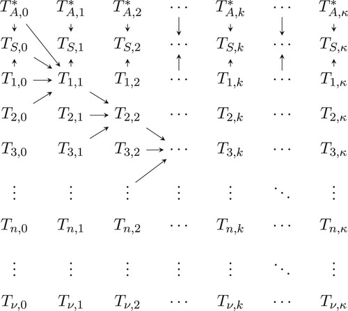
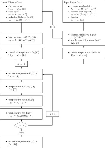
Figure 4. Flowchart of the FTCS scheme with a mixed boundary condition, with $0\le k\le \kappa$ and $S=0\le n\le \nu$.

3.2. Implementation

Figure 4 shows the flowchart of the FTCS scheme with a mixed boundary condition, with $0\le k\le \kappa$ and $S=0\le n\le \nu$. For numerical computation and implementation the input data are divided into two groups (data frames), the time-dependent climate-data, which defines the time step $\mathrm{\Delta }t$, and the location-dependent layer-data. With the wind speed u the heat transfer coefficient for every time step k $h_0-h_{\kappa }$ [$\mathrm{W}\cdot {\mathrm{m}}^{-2}\cdot {\mathrm{K}}^{-1}$] is given by Equation (11(11) $h\left(t\right)=10\cdot (0.174+0.941\cdot u(t{)}^{0.366})$(11) ). Further, this leads to the virtual air temperature $T_{A,0}^{\ast }-T_{A,\kappa }^{\ast }$ for every time step k with Equation (15(15) $h\cdot (T_A^{\ast }-T_S)=h\cdot (T_A-T_S)+Q$(15) ). With the layer-data of every layer i the thermal diffusivity ${\alpha }_i$ is given by Equation (2(2) $\alpha =\frac{\lambda }{c\cdot \rho }$(2) ). This leads, together with the time step size $\mathrm{\Delta }t$ from the climate-data input, to a stable layer thickness $\mathrm{\Delta }{x}_i$. For accurate simulations each layer i needs to be divided into j sublayers with $\mathrm{\Delta }{x}_j>\mathrm{\Delta }{x}_i$, where $\mathrm{\Delta }{x}_j$ is the thickness of the sub-layer. By setting the sublayer thickness, the position of the interfaces is defined and the initial temperature profile can be chosen. For long-term simulations the failure of the chosen initial temperature will be neglected. Now both data frames are preset for the pre-described simulation.

3.3. Input data

Necessary input parameters to compute the temperature profiles are: (i) air temperature (ambient temperature), (ii) wind speed, (iii) solar radiation, (iv) vapor pressure, (v) subgrade temperature, (vi) initial temperature profile, (vii) geometry, (viii) thermophysical material parameters and (ix) pavement surface properties.

Actual hourly data of air temperature, wind velocity, solar radiation and vapor pressure are needed to define the upper boundary condition when the surface temperature is unknown (Equation (17(17) $T_{S,k+1}=-\frac{T_{A,k+1}^{\ast }-T_{1,k+1}}{\left(\frac{\lambda }{h_{k+1}}+\frac{\mathrm{\Delta }x}{2}\right)}\cdot \frac{\lambda }{h_{k+1}}+T_{A,k+1}^{\ast }$(17) ) and Equation (18(18) $T_{1,k+1}=a\cdot \frac{\mathrm{\Delta }t}{\mathrm{\Delta }{x}^2}\cdot \left[T_{2,k}-2\cdot T_{1,k}-\frac{T_{A,k}^{\ast }-T_{S,k}}{\frac{\lambda }{h_k}}\cdot \left(\frac{\lambda }{h_k}-\frac{\mathrm{\Delta }x}{2}\right)+T_{A,k}^{\ast }\right]+T_{1,k}$(18) )).

As aforementioned, in Eberhardsteiner et al. (2016) and Bayraktarova et al. (2017) it was found that the solar radiation has a great impact on the surface temperature. The proposed temperature prediction model uses measured solar radiation data, which is only rarely available in Austria. However, there are some empirical equations, that either estimate the solar radiation based on the solar constant and the location of the sun or use cosine functions. Some of them also consider the effect of cloud cover by using quantified parameters. These equations are summarised in Chen et al. (2019). Most of these equations have been derived based on statistical analysis and are database- and region-dependent. For this reason their applicability in Austria has to be examined.

The pavement surface properties – albedo and emissivity have to be cautiously determined, in order to calculate the radiation balance. A summary of typical values of these parameters is given in Chen et al. (2019).

The lower boundary condition in the presented method is the ground temperature at 2 m depth. Typical ground temperatures for different climatic periods in Austria are given by Wistuba (2003) with (24) $\begin{array}{rl}y\left(x\right)& :=1.19\cdot {10}^{-3}\cdot x^5-4.02\cdot {10}^{-2}\cdot x^4+4.3\cdot {10}^{-1}\cdot x^3\\ & -1.42\cdot x^2-1.55\cdot {10}^{-1}\cdot x+1.02\cdot 10\end{array}$(24) where $1\le x\le 12$ (Months).

Measurements of the ground temperature at a depth of 2 m at two places with various sea levels, ground conditions and climatic region in Austria show the same annual temperature profile (Wistuba 2003). Another study (Qin and Hiller 2011) confirmed that the ground temperature is strongly affected by the heat flow from the interior of the earth and for this reason exhibits fewer variations.

The chosen initial temperature profiles are based on long-therm ground-temperature measurements (from 1961 to 1990) at measuring station Kremsmünster/Upper Austria. Thereby, the average ground temperature at different depths was implemented (Table 2).

Table 2. Initial temperature profiles for the six climate periods at various depths (Wistuba 2003).

Period	Date	Temperature (${}^{\circ }$C) at depth (cm)
		2	10	20	30	50	100	200
1	December 16–March 15	2.4	2.7	2.9	3.0	3.8	5	7.6
2	March 16–May 15	9.6	9.0	8.4	7.9	8.0	7.0	6.3
3	May 16–June 15	17.1	16.2	15.4	14.7	14.2	11.8	8.7
4	June 16–September 15	17.6	17.0	16.7	16.4	16.1	14.7	12.3
5	September 16–October 15	13.5	13.7	13.9	14.1	14.4	14.6	14.4
6	October 16–December 15	5.8	6.5	7.1	7.4	8.2	9.8	12.1

3.4. Validation of the model

Since the FDM is a simulation with approximate approaches, a validation was carried out comparing measured temperature profiles with simulated temperature profiles. Data was collected from two measuring stations in Austria: (i) in Wopfing on a test track and (ii) on the highway A2 near Baden at km 21.

The test track in Wopfing consists of 130 mm thick concrete slabs, a 150 mm thick upper base layer and a 150 mm thick lower base layer. The measured hourly data from Wopfing includes air temperature, wind velocity, relative air humidity, global solar radiation, pavement surface temperature and temperature at a depth of 130 mm. The data acquisition lasted 10 months (from 25 December 2015 to 23 October 2016). Using this data, material properties from Table 3, an albedo of 0.45 and an emission coefficient of 0.88 the temperature distribution has been simulated with the proposed model. The values of the parameters albedo and emission coefficient have been adapted to give a good correspondence between measured and simulated surface temperature as in Figures 5 and 6 shown.

Figure 5. Comparison of measured and predicted surface temperatures in the summer, weather data from Wopfing.

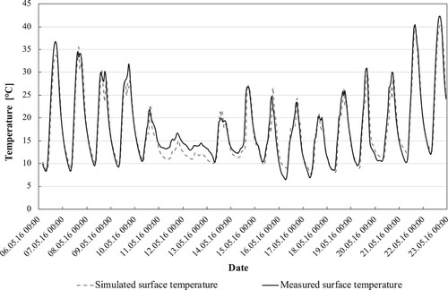
Figure 6. Comparison of measured and predicted surface temperatures in the winter, weather data from Wopfing.

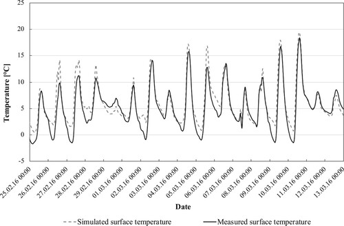
Table 3. Material properties.

Parameter	Units	Concrete slab	Asphalt layer	Base layer	Ground (gravel)
Density	$\mathrm{k}\mathrm{g}\cdot {\mathrm{m}}^{-3}$
• Dry		2370	2120	1800	2100
• Water-saturated		2370	2120	2300	2100
Specific heat capacity	$\mathrm{k}\mathrm{J}\cdot {\mathrm{k}\mathrm{g}}^{-1}\cdot {\mathrm{K}}^{-1}$
• Dry		0.78	0.92	0.72	0.94
• Water-saturated		0.78	0.92	1.13	1.80
Thermal conductivity	$\mathrm{W}\cdot {\mathrm{m}}^{-1}\cdot {\mathrm{K}}^{-1}$
• Dry		1.60	0.70	0.40	0.50
• Water-saturated		1.60	0.70	1.40	2.50
Reference		FGSV (1994)	FGSV (1994)	VDI (2001)	VDI (2001)

Differences up to 4 K arise when comparing both temperature plots. It is obvious from Figures 5 and 6 that the temperature prediction is more accurate for the summer than for the winter. This means that different sets of the parameters, defining the heat flux at the upper boundary, has to be used depending on the weather conditions (e.g. snow, freeze and thaw, the degree of water saturation). Hermansson (2004) studied extensively this effect and developed a model that changes automatically between summer and winter values for these parameters. The change is based on air temperature and solar radiation only. An evaluation of such weather data from multiple weather stations must be performed to define such limit values for Austria. Due to lack of sufficient weather data, this was not implemented in the proposed model.

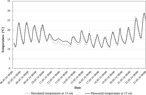
In addition, a comparison of the temperature plots at 130 m depths (Figure 7) shows differences up to 3 K, which demonstrate the accuracy of the proposed temperature prediction model. It appears that the temperature at the top nodes on the pavement surface is more affected by the ambient temperature variation than the temperature at the bottom nodes. This trend was also confirmed by Ali and Urgessa (2012).

Figure 7. Comparison of measured and predicted temperatures at 130 mm depth, weather data from Wopfing.

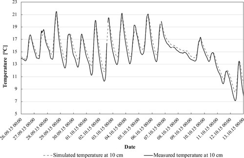
Furthermore, to verify the accuracy of the proposed method using only the surface temperature as an input, the temperature distribution within a concrete layer on the highway A2 near Baden at km 21 was measured every hour over a one-year period at 4 depths (at 50, 100, 150 and 200 mm distance from the surface) and on the surface. The pavement structure consists of a 250 mm concrete slab, 50 mm asphalt layer and 450 mm base layer.

Figure 8 shows a very good agreement between the measured and simulated values with a maximum discrepancy of 2 K. This agreement indicates an adequate accuracy of the proposed temperature prediction model by using actual surface temperatures.

Figure 8. Comparison of measured and predicted temperatures (with surface temperature) at 100 mm depth, weather data from highway A2.

3.5. Simulations and results

Hourly surface temperature data from 16 measuring stations distributed over the Austrian rigid highway pavement network obtained from 2011 to 2015 was utilised for the simulation of the temperature distribution and the establishment of representative temperature gradients. The data was collected and provided by the Austrian highway authority ASFINAG. This was done because there is no data on countrywide solar radiation and the simulation of temperature profiles in pavements with surface temperature is more accurate.

Within this section, the results from the simulations of the temperature distribution for dry and water-saturated unbound layers with surface temperature data from the 16 above-mentioned measuring stations are discussed.

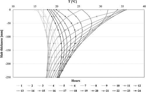
The following Figure 9 shows typical temperature distributions at various times of the day in a concrete slab with a thickness of 250 mm, obtained as a result from the simulations using the proposed temperature prediction model. A strong inward curvature of the temperature profile indicates high-temperature gradients. As in Figure 9 compared, the temperature gradients are positive during day time and negative during night time. However, in Eberhardsteiner et al. (2016) and Bayraktarova et al. (2017) was concluded that the negative temperature gradients, which occur during the night time have an insignificant impact on the maximum curling stresses and, therefore, were not considered in pavement design.

Figure 9. Predicted hourly temperature profiles at measuring Station Kematiger-Berg, 17 June 2014.

Figure 10 shows another comparison between the resulting temperature gradients estimated with thermophysical material parameters of dry and water-saturated unbound layers. The resulting temperature gradients from water-saturated unbound layers tend to be higher during the warm periods and lower during the cold periods. This can be explained by the fact that water-saturated layers have greater thermal conductivities than dry layers. This trend can also be seen in Table 4, where the 95th percentile was estimated based on the resulting temperature gradients from measuring station Inzersdorf in eastern Austria for the six climate periods during four years (2011 to 2014). Due to the lack of soil moisture data for the evaluated stations, the final value of the temperature gradient for each period is generated as a mean value of the temperature gradients from dry and water-saturated layers.

Figure 10. Temperature gradients estimated with thermophysical parameters of dry and water-saturated layers: (a) winter day (17 February 2014), (b) summer day (17 June 2014).

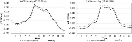
Table 4. Temperature gradients for measuring station Inzersdorf.

		Temperature gradients $\mathrm{\Delta }T$ (K/mm) for different climate periods
		1	2	3	4	5	6
Year	Unbound layers	16.12–15.03	16.03–15.05	16.05–15.06	16.06–15.09	16.09–15.10	16.10–15.12
2014	Dry	0.022	0.063	0.079	0.067	0.040	0.020
	Water-saturated	0.021	0.068	0.090	0.075	0.041	0.020
2013	Dry	0.024	0.063	0.070	0.066	0.005	0.020
	Water-saturated	0.022	0.069	0.078	0.075	0.006	0.019
2012	Dry	0.020	0.062	0.064	0.062	0.045	0.021
	Water-saturated	0.019	0.068	0.071	0.072	0.046	0.019
2011	Dry	0.029	0.058	0.071	0.060	0.047	0.021
	Water-saturated	0.027	0.064	0.080	0.068	0.050	0.018

As the differences in the temperature gradients for each year and station were insignificant, it was concluded to summarise the resulting gradients for each climate period with the mean value of each year of each measuring station. Table 5 shows the summarised temperature gradients for the six climate periods, which were statistically analysed with the 95th, 75th and 50th percentiles. Depending on the road category, a different percentile can be chosen to account a representative proportion for the calculation of curling stresses and for the design life of the pavement structure.

Table 5. Temperature gradients for the six climate periods, evaluated with different percentiles.

	Temperature gradients $\mathrm{\Delta }T$ (K/mm) for different climate periods
	1	2	3	4	5	6
Percentile	16.12–15.03	16.03–15.05	16.05–15.06	16.06–15.09	16.09–15.10	16.10–15.12
95th	0.023	0.070	0.83	0.076	0.045	0.020
75th	0.010	0.042	0.051	0.045	0.024	0.009
50th	0.002	0.023	0.030	0.024	0.011	0.001

4. Impact of the temperature gradients on the design life of the rigid pavement

4.1. Design example

To analyse the impact of the chosen evaluation percentile for the representative temperature gradients on the design life of rigid pavement structures, a design example was performed according to the new Austrian MEPDR method (Eberhardsteiner et al. 2016, 2018; FSV 2020). The obtained results are compared to those resulting from the Austrian standard design catalogue given in the national standard RVS 03.08.63 (FSV 2016). For the purpose of this investigation, a typical highway pavement structure (BE 1, LK 40) was analysed, consisting of 250 mm thick concrete layer with a slab size of $5\times 5$  m and a bending tensile strength of 5.27 MPa, 50 mm asphalt layer and 450 mm unbound gravel layer (Table 6). The load transfer between individual slabs is realised by standard dowels with a diameter of 25 mm, length of 500 mm and dowel spacing of 300 mm. Various bearing capacities of the base and the subgrade layers were used depending on the seasonal period (P1, P2, P3 and P4). Traffic loads are estimated using representative distributions for the occurrence of heavy goods vehicle (HGV) types, gross vehicle weights and axles loads (Eberhardsteiner and Blab 2017). To account for seasonal temperature variations, different percentiles of the representative temperature gradients (Table 6) were used.

Table 6. Inputparameters for the design example.

	Pavement structure BE1, according to RVS 03.08.63 (FSV 2016), slab size $5\times$5 m
Layer	E-Modulus (MPa)				ν	Thickness (mm)
Concrete slab	30,000				0.17	250
Asphalt	3500				0.40	50
	P1	P2	P3	P4
Base layer	678	169	242	339	0.35	450
Subgrade	280	70	100	140	0.35	–

Considering these input parameters, plate theory according to Kirchhoff (Höller et al. 2019) is applied to determine the resulting stresses due to traffic loads for each axle of each vehicle and each subgrade period. Then, the further developed Eisenmann's model (Houben 2009) is used for the estimation of the curling stresses for the six climate periods.

In another step, the allowable number of cycles the pavement is able to resist $N_{ijk}$ (resistance) can be determined for each axle i of each vehicle j and each climate period k by applying Smith's fatigue criteria (Eisenmann and Leykauf 2003): (25) $\log N_{ijk}=\frac{\frac{{\sigma }_{tr}+{\sigma }_c}{f_{ct\left(ben\right)}}-0.8}{0.0875\frac{{\sigma }_c}{f_{ct\left(ben\right)}}-0.07}$(25) where ${\sigma }_{tr}$ is the stress due to traffic $\left[\mathrm{N}\cdot {\mathrm{m}\mathrm{m}}^{-2}\right]$, ${\sigma }_c$ is the curling stress $\left[\mathrm{N}\cdot {\mathrm{m}\mathrm{m}}^{-2}\right]$ and $f_{ct\left(ben\right)}$ is the bending tensile strength $\left[\mathrm{N}\cdot {\mathrm{m}\mathrm{m}}^{-2}\right]$. The corresponding damage $C_{ijk}$ is given by (26) $C_{ijk}=\frac{1}{N_{ijk}}.$(26) The average damage $C_{\mathrm{r}\mathrm{e}\mathrm{s}}$ is provided by (27) $C_{res}=\sum _i\sum _j\sum _k{p}_j\cdot p_k\cdot C_{ijk}$(27) in which $p_j$ is the appearance probability of vehicle j on the HGV traffic volume and $p_k$ is the relative duration of climate period k during one year. Hence, the number of load cycles the pavement is able to resist, $N_{\mathrm{r}\mathrm{e}\mathrm{s}}$, reads as (28) $N_{res}=\frac{1}{C_{res}}$(28) For the considered road section, the number of the expected load passages $N_{\mathrm{i}\mathrm{m}\mathrm{p}}$ (impact) was estimated using the following equation: (29) $N_{imp}=\text{ AADTT}\cdot V\cdot S\cdot 365\cdot n\cdot z$(29) and assuming an annual average of the overall daily heavy traffic (AADTT) of 2000 HGVs/ 24 h, a factor V related to the distribution of vehicles to several lanes $(V=1)$, a factor S considering the loading distribution of vehicle tracks within one lane $(S=1)$, a 30-years design life n, an annual traffic growth of 2% and a growth factor z (30) $z=\frac{q^n-1}{n\cdot (q-1)}$(30) where $q=1+p/100$, and p denotes the annual traffic growth rate in %.

Within this design process (according to the serviceability limit state), the number of load cycles the pavement is able to resist $N_{\mathrm{r}\mathrm{e}\mathrm{s}}$ (resistance), is related to the expected number of passages during the design life, $N_{\mathrm{i}\mathrm{m}\mathrm{p}}$ (impact), by Equation (31(31) $\frac{N_{imp}}{N_{res}}\le 1.$(31) ) (31) $\frac{N_{imp}}{N_{res}}\le 1.$(31)

4.2. Analysis of the results

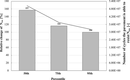
Figure 11 shows the impact of the chosen temperature gradient percentile on the design life. Since the temperature gradients evaluated with lower percentile are low (Table 5), the allowable number of cycles the pavement is able to resist $N_{\mathrm{r}\mathrm{e}\mathrm{s}}$ increase with decreasing percentile. The grey bars in Figure 11 show the relative change of $N_{\mathrm{r}\mathrm{e}\mathrm{s}}$ assuming that 100% corresponds to 95th percentile. $N_{\mathrm{r}\mathrm{e}\mathrm{s}}$ rises by up to 57% when applying temperature gradients evaluated with the 50th percentile.

Figure 11. Allowable number of load repetitions estimated by using different temperature gradient percentiles and their relative change.

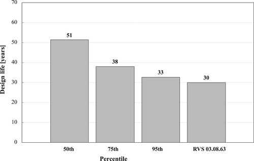
The predicted design lives using the new MEPDR and temperature gradients evaluated with different percentiles are compared with the design life obtained from the traditional design catalogue RVS 03.08.63 (FSV 2016) in Figure 12. Applying the MEPDR results in an increase of calculated technical lifetime up to 21 years (50th percentile of temperature gradients) compared to the traditional design catalogue. These results can be explained by the fact that the design life obtained from the design catalogue has been estimated with a constant temperature gradient during the whole year. Furthermore, the detailed characterisation of the climatic boundary conditions leads to a more accurate prediction of the design life.

Figure 12. Comparison between the design lives estimated by using different temperature gradient percentiles.

5. Conclusion

The main purpose of the current study was to develop an easily adaptable method to account for the seasonal temperature variations in the design of rigid pavements. For this reason, a temperature prediction model was implemented in a tool, validated and used to derive realistic temperature gradients representing the climatic conditions in Austria. The temperature gradients are used as input parameter for the estimation of resulting curling stresses. The proposed procedure is practical and much simpler in comparison to the procedure implemented in the MEPDG. It uses the information readily available in Austria and can be easily adapted for other locations.

The analysis of simulated temperature profiles shows that the temperature gradients estimated with data from dry unbound layers tend to be higher during the cold periods and lower during the warm periods compared to water-saturated layers. This indicates the importance of incorporating soil moisture data in the simulation of temperature distribution in pavement structures. The results of statistical analysis of the temperature gradients allow for choosing a different temperature gradient percentile depending on the road category and on the specific local climatic conditions. The main finding from the demonstrated design example is that the more detailed the characterisation of climatic boundary conditions is, the more accurate is the prediction of the design life.

Acknowledgements

The authors gratefully acknowledge financial support from the Austrian Research Promotion Agency (FFG) through project 'OBESTAS – Optimized design of rigid pavement constructions.

Disclosure statement

No potential conflict of interest was reported by the author(s).

References

- ABAQUS/Standard, 2014. User's manual, version 6.14. Dassault Systèmes Simulia Corp, Online Database.
- Alavi, M., Pouranian, M., and Hajj, E., 2014. Prediction of asphalt pavement temperature profile with finite control volume method. Transportation Research Record: Journal of the Transportation Research Board, 2456, 96–106.
- Ali, W., and Urgessa, G., 2012. Numerical prediction model for temperature distributions in concrete at early ages. American Journal of Engineering and Applied Sciences, 5 (4), 282–290.
- Barber, E.S., 1957. Calculation of maximum pavement temperatures from weather reports. Bulletin 168 Washington, D.C.: Highway Research Board, 1–8.
- Bayraktarova, K., Eberhardsteiner, L., and Blab, R. 2017. Seasonal temperature distribution in rigid pavements. In: A. Loizos, I. Al-Qadi and S. T., eds. Proceedings of the 10th international conference on the bearing capacity of roads, railways and airfields (BCRRA 2017), 28–30 June 2017, Athen. CRC Press, 2087–2093.
- Beckemeyer, C.A., Khazanovich, L., and Yu, H.T., 2002. Determining amount of built-in curling in jointed plain concrete pavement: case study of Pennsylvania I-80. Transportation Research Record, 1809, 85–92.
- Bradbury, R., 1938. Reinforced concrete pavements. University of Wisconsin – Madison: Wire Reinforcement Institute.
- Caliendo, C., and Parisi, A., 2010. Stress-prediction model for airport pavements with jointed concrete slabs. Journal of Transportation Engineering, 136 (7), 664–677.
- Chandrappa, A., and Biligiri, K., 2015. Development of pavement-surface temperature predictive models: parametric approach. Journal of Materials in Civil Engineering, 28 (3), 04015143.
- Chen, J., Wang, H., and Xie, P., 2019. Pavement temperature prediction: theoretical models and critical affecting factors. Applied Thermal Engineering, 158, 1–14.
- Choubane, B., and Tia, M., 1995. Analysis and verification of thermal-gradient effects on concrete pavement. Journal of Transportation Engineering, 121 (1), 75–81.
- Dempsey, B.J., Herlache, W., and Patel, A., 1985. Climatic-m-structural pavement analysis program. Transportation Research Record, 1095, 111–123.
- Dempsey, B. and Thompson, M., 1970. A heat transfer model for evaluating frost action and temperature related pavements effects in multi-layered pavement systems. Highway Research Record, 342, 39–56.
- Diefenderfer, B., Al-Qadi, I., and Diefenderfer, S., 2002. Model to predict pavement temperature profile: development and validation. Journal of Transportation Engineering, 132, 162–167.
- Eberhardsteiner, L., etal, 2016. OBESTAS – Optimierte Bemessung starrer Aufbauten von Straßen. Vienna: Vienna University of Technology, Institute of Transportation.
- Eberhardsteiner, L., and Blab, R., 2017. Design of bituminous pavements: a performance-related approach. Road Materials and Pavement Design, 20 (2), 244–258.
- Eberhardsteiner, L., Foltin, K., Bayraktarova, K., and Blab, R., 2018. Performance-related approach for rigid pavement design. In: E. Masad, A. Bhasin, T. Scarpas, I. Menapace and A. Kumar, eds. International conference on advances in materials and pavement performance prediction (AM3P 2018), 16–18 April 2018, Doha. CRC Press, 457–461.
- Eisenmann, J., 1979. Concrete pavements – design and construction (in German). München: Wilhelm Ernst and Sohn.
- Eisenmann, J., and Leykauf, G., 1990. Simplified calculation method of slab curling caused by shrinkage. In: A. Loizos, I. Al-Qadi and S. T., eds. 2nd international workshop on theoretical design of concrete pavements, Madrid, Spain.
- Eisenmann, J., and Leykauf, G., 2003. Concrete pavements – design and construction (in German). München: Ernst and Sohn.
- FGSV, 1994. Entstehung und Verhütung von Frostschäden an Straßen. Bonn: FGSV.
- FSV, 2016. RVS 03.08.63: Oberbaubemessung. Vienna: FSV.
- FSV, 2020. RVS 03.08.69: Rechnerische Dimensionierung von Betonstraßen. Vienna: FSV.
- Gao, X., Wei, Y., and Huang, W., 2017. Strain-based equivalent temperature gradient in concrete pavement and comparaisson with other quantification methods. Journal of Transportation Engineering, 18, 00–00.
- Geiger, R., 1959. The climate near the ground. Cambridge: Harvard University Press.
- Hermansson, A., 2002. Simulation of asphalt concrete (AC) pavement temperatures for use with FWD. Road Materials and Pavement Design, 3, 281–297.
- Hermansson, A., 2004. Mathematical model for paved surface summer and winter temperature: comparison of calculated and measured temperatures. Cold Regions Science and Technology, 40, 1–17.
- Hiller, J., and Roesler, J., 2010. Simplified nonlinear temperature curling analysis for jointed concrete pavements. Journal of Transportation Engineering, 136, 654–663.
- Höller, R., Aminbaghai, M., Eberhardsteiner, L., Eberhardsteiner, J., Blab, R., Pichler, B., and Hellmich, C., 2019. Rigorous amendment of Vlasov's theory for thin elastic plates on elastic Winkler foundations, based on the principle of virtual power. European Journal of Mechanics – A/Solids, 73, 449–482.
- Houben, L., 1992. Finite element analysis of plain concrete pavements (V): comparison with the Eisenmann theory. Journal 'BetonwegenNieuws, 88, 16–23.
- Houben, I.L.J.M., 2009. Structural design of pavements. Available from: http://www.citg.tudelft.nl/en/about-faculty/departments/structural-engineering/sections/pavement-engineering/education/lectures/.
- Huang, K., et al., 2017. A developed method of analyzing temperature and moisture profiles in rigid pavement slabs. Construction and Building Materials, 151, 782–788.
- Ioannides, A., and Khazanovich, L., 1998. Nonlinear temperature effects on multilayered concrete pavements. Journal of Transportation Engineering, 124 (2), 128–136.
- Jeong, J.H., and Zollinger, D., 2006. Finite-element modeling and calibration of temperature prediction of hydrating Portland cement concrete pavements. Journal of Materials in Civil Engineering, 18 (3), 317–324.
- Khazanovich, L., et al., 2001. Development of rapid solutions for reinforced concrete pavement stresses. Transportation Research Record: Journal of the Transportation Research Board, 1778, 64–72.
- Krebs, H. and Böinger, G., 1981. Temperaturberechnungen am bituminösen Straßenkörper. Heft 347. Forschung Straßenbau und Straßenverkehrstechnik Bonn-Bad Godesberg.
- Krsmanc, R., Slak, A.S., and Demsar, J., 2013. Statistical approach for forecasting road surface temperature. Meteorological Applications, 20, 439–446.
- Linke, F. and Möller, F., 1974. Handbuch der Geophysik. Stuttgart: Gebrüder Borntraeger.
- McCullough, B., and Rasmussen, R., 1999. Fast-track paving: concrete temperature control and traffic opening criteria for bonded concrete overlays, volume 1: final report. Austin, TX: FHWA, US Department of Transportation.
- Minhoto, M., et al., 2005. Predicting asphalt pavement temperature with a three-dimensional finite element method. Transportation Research Record, 1919 (1), 96–110.
- Mohamed, A., and Hansen, W., 1996. Prediction of stresses in concrete pavements subjected to non-linear gradients. Cement and Concrete Composites, 18 (6), 381–387.
- NCHRP, 2004. Guide for mechanistic-empirical design of new and rehabilitated pavement structures. Washington, DC.
- Qin, Y., 2016. Pavement surface maximum temperature increases linearly with solar absorption and reciprocal thermal inertial. International Journal of Heat and Mass Transfer, 97, 391–399.
- Qin, Y., and Hiller, J.E., 2011. Modeling the temperature and stress distributions in rigid pavements: impact of solar radiation absorption and heat history development. KSCE Journal of Civil Engineering, 15 (8), 1361–1371.
- Rao, S., and Roesler, J.R., 2005. Characterising effective built-in curling from concrete pavement field measurements. Journal of Transportation Engineering, 131 (4), 320–327.
- Sherif, A., and Hassan, Y., 2004. Modelling pavement temperature for winter maintenance operations. Canadian Journal of Civil Engineering, 31 (2), 369–378.
- Siddique, Z.Q., Hossain, M., and Meggers, D., 2005. Temperature and curling measurements on concrete pavement. In: The 2005 mid-continent transportation research symposium, 18–19 August 2018, Ames Iowa.
- Solaimanian, M., and Kennedy, T., 1993. Predicting maximum pavement surface temperature using maximum air temperature and hourly solar radiation. Transportation Research Record, 1417, 1–11.
- Teltayev, B., and Koblanbek, A., 2015. Modeling of transient temperature distribution in multilayer asphalt pavement. Geomechanics and Engineering, 8, 133–152.
- Thomlinson, J., 1940. Temperature variations and consequent product by daily and seasonal temperature cycles in concrete slabs. Concrete Constructional Engineering, 36, 298–307.
- VDI, 2001. VDI 4640: Thermische Nutzung des Untergrunds – Grundlagen, Genehmigungen, Umweltaspekte – Blatt 1. Düsseldorf: VDI.
- Wang, D., 2012. Analytical approach to predict temperature profile in a multilayered pavement system based on measured surface temperature data. Journal of Transportation Engineering, 138 (5), 674–679.
- Wang, D., 2016. Prediction of time-dependent temperature distribution within the pavement surface layer during FWD testing. Journal of Transportation Engineering, 142 (7), 06016002.
- Wang, D., and Roesler, J., 2014. One-dimensional temperature profile prediction in multi-layered rigid pavement systems using a separation of variables method. International Journal of Pavement Engineering, 15 (5), 372–382.
- Wang, D., Roesler, J., and Guo, D., 2009. Analytical approach to predicting temperature fields in multilayered pavement systems. Journal of Engineering Mechanics, 135 (4), 334–344.
- Wistuba, M., 2003. Climatic influences on asphalt pavements: Determining the design temperature for the Austrian analytical pavements design. Heft 15. Vienna University Technology, Institute frustration, Research Center of Road Engineering.
- Yavuzturk, C., Ksaibati, K., and Chiasson, A., 2005. Assessment of temperature fluctuations in asphalt pavements due to thermal environmental conditions using a two-dimensional, transient finite-difference approach. Journal of Materials in Civil Engineering, 17 (4), 465–475.
- Yu, H.T., Khazanovich, L., Darter, M.I., and Ardani, A., 1998. Analysis of concrete pavement responses to temperature and wheel loads measured from instrumented slabs. Transportation Research Record: Journal of the Transportation Research Board, 1639 (6), 94–101.