An intelligent approach for predicting the strength of geosynthetic-reinforced subgrade soil

ABSTRACT

In the recent times, the use of geosynthetic-reinforced soil (GRS) technology has become popular for constructing safe and sustainable pavement structures. The strength of the subgrade soil is routinely assessed in terms of its California bearing ratio (CBR). However, in the past, no effort was made to develop a method for evaluating the CBR of the reinforced subgrade soil. The main aim of this paper is to explore and appraise the competency of the several intelligent models such as artificial neural network (ANN), least median of squares regression, Gaussian processes regression, elastic net regularisation regression, lazy K-star, M-5 model trees, alternating model trees and random forest in estimating the CBR of reinforced soil. For this, all the models were calibrated and validated using the reliable pertinent historical data. The prognostic veracity of all the tools mentioned supra were assessed using the well-established traditional statistical indices, external model evaluation technique, multi-criteria assessment approach and independent experimental dataset. Due to the overall excellent performance of ANN, the model was converted into a trackable functional relationship to estimate the CBR of reinforced soil. Finally, the sensitivity analysis was performed to find the strength and relationship of the used parameters on the CBR value.

KEYWORDS:

• California bearing ratio
• geosynthetic reinforcement
• subgrade soil
• machine learning
• intelligent predictive modelling

1. Introduction

The pavement design is highly influenced by the load-carrying capacity of the subgrade soil. Geosynthetic reinforcement provides a sustainable and cost-effective way of soil subgrade improvement. The use of geosynthetic reduces the deformation of the pavement caused by the vehicular load, enhancing its strength and durability (Shukla 2002). Starting in the late 1900s, many studies can be found in the literature that investigate the beneficial effects of geosynthetic reinforcement in road construction projects (e.g. Miura et al. 1990, Perkins 1999, Cuelho et al. 2005, Abu-Farsakh et al. 2016, Chen et al. 2018, Singh et al. 2019). The California bearing ratio (CBR) is considered as one of the key parameters used to ascertain the subgrade capacity to withstand the applied traffic loads (ASTM 2016). To date, many researchers have employed the CBR testing to investigate the effects of geosynthetic reinforcement on subgrade material (Duncan-Williams and Attoh-Okine 2008, Naeini and Ziaie-Moayed 2009, Nair and Latha 2011, Choudhary et al. 2012, Rajesh et al. 2016, Mittal and Shukla 2018, Negi and Singh 2019). The advent of soft computing and data-driven modelling has made many traditional approaches antiquated. In recent times, the use of artificial intelligence (AI)/machine learning (ML) techniques has become very common in solving various complex engineering problems including those related to pavement engineering (Nazemi and Heidaripanah 2016, Daneshvar and Behnood 2020, Ghosh Mondal and Kuna 2020, Han et al. 2020, Olowosulu et al. 2020, Ghorbani et al. 2021). The laborious, costly and time-consuming nature of the CBR, and moreover, due to the complex non-linear relationships between the soil properties, many researchers have utilised ML to predict the CBR of the soil. Taskiran (2010) applied artificial neural network (ANN) and gene expression programming (GEP) techniques to learn the non-linear relationships between CBR and various index properties of the fine-grained soils sourced from Southeast Anatolia, Turkey. The maximum dry unit weight (${\gamma }_d$), plasticity index (PI), liquid limit (LL), optimum moisture content (OMC) and the content of different soil fractions were identified as the most effective parameters that influence the CBR values of the soils. Yildirim and Gunaydin (2011) used simple multiple regression and ANN to propose correlations for the preliminary estimation of CBR values of different soil, by employing the results of sieve analysis, Atterberg limits, maximum dry density and OMC. Alawi and Rajab (2013) utilised multiple linear regression (MLR) analysis to predict the CBR of the unreinforced subbase soil layer. Recently, similar applications of advanced ML techniques for the prediction of CBR of different unreinforced soils were also conducted by other researchers (Erzin and Turkoz 2016, González Farias et al. 2018, de Souza et al. 2020, Nagaraju et al. 2020, Tenpe and Patel 2020). Similarly, several studies were also carried out to evaluate permanent deformation and resilient modulus of recycled demolition wastes in pavements using ML algorithms (Arulrajah et al. 2013, Ullah et al. 2020, Ghorbani et al. 2020a). Ghorbani et al. (2020b, 2021) successfully developed an ANN model to predict the permanent strain of blends of two recycled waste materials under different stress and temperature levels and shakedown analysis of polyethylene terephthalate (PET) blend with demolition waste material as the subbase layer of pavement, respectively. However, the review of the current literature revealed that the efforts to predict the CBR of geosynthetic-reinforced subgrade soil are extremely limited. In fact, Singh et al. (2020) is the only study that has attempted to predict the CBR of geogrid-reinforced soil using a fuzzy logic-based modelling technqiue. However, to the best of authors’ knowledge, there is currently no research in the present literature that provides development, implementation and comprehensive comparison of ML-based solutions to the problem of CBR of geosynthetic-reinforced subgrade soil.

In this paper, an attempt is made to predict the CBR of geosynthetic-reinforced soil (GRS) using the data-driven-based ML models. The main objectives of this research are fourfold: (1) assessment of numerous ML models in predicting the CBR of GRS; (2) comprehensive comparison of all the predictive tools utilised for the same problem; (3) suggestion of ANN-based trackable mathematical formula for estimating the CBR of soil reinforced with geosynthetic layers; and (4) independent validation by conducting new CBR tests on reinforced soil.

2. Material and methods

In this work, eight ML models namely, ANN, least median of squares regression (LMSR), Gaussian processes regression (GPR), elastic net regularisation regression (ENRR), lazy K-star (LKS), M-5 model trees, alternating model trees (AMT) and random forest (RF) models, were constructed to predict the CBR of GRS. All the models were simulated using Waikato Environment for Knowledge Analysis (WEKA). It may be noted that in the past, many researchers and scientists have utilised the WEKA framework for function approximation and feature classification (Gao et al. 2019, Moayedi et al. 2020, Olowosulu et al. 2020). Moreover, the new CBR tests were also conducted to ensure the independent validation of the data-driven models and discussed later in the paper.

2.1. Experimental database development and model attributes

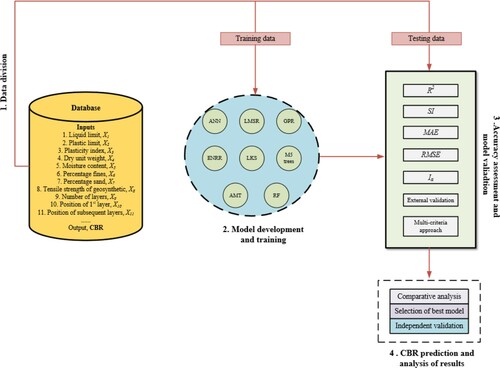
In order to calibrate and validate all the data-driven models, the data set of 97 soaked CBR tests is retrieved from the literature. This includes 4 cases reported by Duncan-Williams and Attoh-Okine (2008), 30 cases reported by Vinod and Minu (2010), 16 cases reported by Choudhary et al. (2011), 2 cases reported by Kuity and Roy (2013), 4 cases each reported by Carlos et al. (2016) and Rajesh et al. (2016), 9 cases by Mittal and Shukla (2018, 2019) and 28 cases by Negi and Singh (2019). The reliability of a model depends upon the comprehensiveness of the input data set. In this study, it was ensured by incorporating a wide variety of soils, ranging between sandy soil (SP) and fine-grained soils (ML, MH, CL and CH), as per the Unified Soil Classification System (USCS). These soils cover a range of engineering properties that affect the stiffness of a soil, such as soil index properties and particle size distribution (Youd 1973, Zheng and Hryciw 2016). However, the geotechnical engineering models that are the most effective in predicting the non-linear soil behaviour are based on the important soil parameters that can be obtained via routine tests (Oztoprak and Bolton 2013). The detail of the utilised database is provided in Table 1. For predicting the output, that is, CBR of GRS, the input parameters include LL (X₁), plastic limit (X₂), PI (X₃), dry unit weight (maximum) (X₄), optimum moisture content (X₅), percentage fines (passing sieve No. 200) (X₆), percentage sand (X₇), tensile strength of geosynthetic reinforcement (X₈), number of reinforcement layers (X₉), position of the first reinforcement layer (X₁₀) and position of the subsequent reinforcement layers (X₁₁). All these parameters were selected based on the fact that the current literature shows that they have an effect on the CBR of reinforced soil.

Table 1. Statistical properties of the data set.

Descriptive stats	Liquid limit	Plastic limit	Plastic Index	Dry unit weight	Optimum moisture content	% Fines	% Sand	Tensile strength of geosynthetic	Number of layers	Position of 1st layer	Position of subsequent layers	CBR
	X1	X2	X3	X4	X5	X6	X7	X8	X9	X10	X11
Mean	50.746	28.612	22.135	15.782	20.986	85.025	14.268	16.821	1.392	0.382	0.101	6.453
Median	46.000	25.000	23.000	15.100	18.000	94.000	6.000	13.000	1.000	0.330	0.000	4.870
Mode	46.000	23.000	23.000	15.100	18.000	97.000	3.000	30.000	1.000	0.200	0.000	3.460
SD	15.452	8.670	7.787	2.351	7.709	22.826	22.344	11.901	0.701	0.210	0.176	6.183
Kurtosis	1.751	1.565	0.666	−1.143	−0.808	3.783	3.956	−1.207	3.214	−0.478	2.111	10.454
Skewness	−0.837	−0.837	−0.878	0.076	0.805	−2.242	2.285	0.423	1.881	0.780	1.669	3.122
Range	71	39	32	8.25	26.8	83.8	82	39.17	3	0.68	0.66	32.7
Minimum	0	0	0	12.54	8.2	16.2	0	2.81	1	0.15	0	1.3
Maximum	71	39	32	20.79	35	100	82	41.98	4	0.83	0.66	34
Count	97	97	97	97	97	97	97	97	97	97	97	97

SD stands for standard deviation

The developed models were also tested for the independent data set obtained by conducting new CBR tests (AS 1289.6.1.1 2014). It is noteworthy that these data are not a part of the actual database utilised to construct the ML models. Non-plastic sandy soil extracted from the pit site located in the northern region of Perth, Australia, was used during the experimental tests. The properties of the soil and geosynthetic (geotextile) are summarised in Table 2. To evaluate the effect of geosynthetic reinforcement on the strength of the subgrade soil, a total of six CBR tests were performed by varying the depth ratio of the first reinforcement layer (u/H), number of reinforcement layers (N) and depth ratio of the subsequent layer (h/H), where H represents the total height of mould. The proposed scheme of the CBR tests is summarised in Table 3.

Table 2. Properties of soil and geosynthetic material

Soil properties	Magnitude	Geosynthetic properties^a	Magnitude
Maximum dry unit weight (kN/m^3)	17.3	Tensile strength, MD (kN/m)	30
Minimum dry unit weight (kN/m^3)	15.4	Tensile strength, XMD (kN/m)	30
Median grain size (mm)	0.25	Mass (g/m^2)	150
Effective grain size (mm)	0.17	Elongation strain, MD (%)	20
Optimum moisture content (%)	11.8	Elongation strain, XMD (%)	15
Atterberg’s limit	NP
Fines (%)	4.5
Sand content (%)	95.5

Note: NP stands for non-plastic; MD stands for machine direction; XMD stands for cross-machine direction.

^a Provided by the manufacturer.

Table 3. Experimental scheme of the CBR tests

Experiment number	Number of layers (N)	Depth of first layer (u/H)	Depth of subsequent layer (h/H)	CBR (%)
1	1	0.25	0	23.62
2	1	0.50	0	21.98
3	1	0.75	0	17.37
4	2	0.25	0.25	29.3
5	2	0.25	0.5	28
6	2	0.50	0.25	25.88

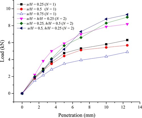
The reinforcement layer was cut into a circular disk with the diameter slightly smaller than the diameter of the mould. In order to fill the mould, dry weight calculations are done based on the maximum dry unit weight of soil and volume of mould. The soil was mixed thoroughly by adding the water content corresponding to OMC. Thereafter, the mould is filled with the soil by placing the geotextile layer at a predetermined depth as reported in Table 3. The test setup with the schematic diagram of the specimen in the CBR test and the placement of geosynthetic at a predetermined depth in the CBR mould is illustrated in Figure 1. The CBR tests were conducted after soaking the sample in water for 96 h. The surcharge load was applied to the specimen to ensure the effect of the thickness of the overlying layer. Load was applied at 1.25 mm/min (moveable base) and the corresponding penetration was measured through the electronic displacement transducer. The load readings were taken at penetrations ranging from 0.5 to 12.5 mm. The CBR values were estimated by taking the load corresponding to 2.5 or 5.0 mm penetration, whichever is the highest as suggested by the relevant standard. Figure 2 depicts the load–penetration curves obtained for the CBR tests of reinforced soil.

Figure 1. Experimental setup for the CBR tests conducted in this study: (a) schematic diagram of the specimen; (b) layout/placement of reinforcement layer at a predetermined depth in CBR mould; (c) test apparatus.

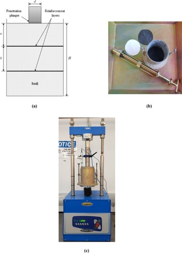
Figure 2: Load–penetration curves of GRS.

2.2. Methodological background of machine learning models

The first and foremost step before mapping the response of any data-driven model is the database partitioning. For this, the data are needed to be randomly divided into training and testing subsets. In this study, 60% of the collected data were randomly chosen for training the ANN, LMSR, GPR, ENRR, LKS, M-5 model trees, AMT and RF models. Thereafter, the predictive veracity of each model was appraised against the remaining 40% of the data set (test data). Moreover, all the data sets have been normalised [−1,1] before feeding it to the model networks, so that each variable would get the same attention during the training process. The brief methodological background of all the data-driven-based modelling techniques utilised to estimate the CBR of reinforced soil is explained in this section. For a more comprehensive understanding, the research scheme employed in this study is also illustrated in Figure 3.

Figure 3. Research scheme employed for estimating the CBR of reinforced soil.

2.2.1. Artificial neural network

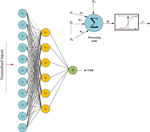
ANN is the well-established and widely recognised ML model used for mapping the non-linear response of any system (Moayedi and Hayati 2018). At its core, the ANN model architecture consists of three parts, namely input layer, one or more hidden layers and output layer. Each layer consists of set processing elements called nodes (neurons) which interact with each other through weighted connections. The computation process can be described as follows: (a) data are presented to the model through input layer nodes; (b) in the hidden–output layer, the data are multiplied by the weight matrix and added to the threshold (bias) vector, thereafter the activation function is applied; (c) output of the hidden layer is mapped as the final outcome after passing through the output layer. Mathematically, for n inputs, the output y is computed as follows (Bishop 2006): (1) $y=f\left(\sum _{i=1}^n{X}_i{w}_i+{\theta }_{\mathrm{o}}\right)$(1) where w is the weight connection and θ is the bias/threshold.

In this study, the sigmoid activation function is used in the hidden layer and given as follows (Han and Moraga 1995): (2) $\mathrm{s}\mathrm{i}\mathrm{g}\left(X\right)=\frac{1}{1+{\mathrm{e}}^{-x}}$(2) For training the neural network, the optimisation procedure suggested by Soleimanbeigi and Hataf (2006) was adopted to select the optimum number of hidden layer nodes. For this, the hidden layer nodes were increased until no further improvement was obtained over the testing data set. Figure 4 illustrates the optimisation process for selecting the number of hidden nodes. It can be observed that the lowest mean absolute error (MAE = 1.233) and root mean square error (RMSE = 1.70) is obtained at nine hidden nodes. However, the model with six hidden nodes is selected as the optimum model as it has less weight connections, but its performance is closer to nine hidden nodes with MAE and RMSE values of 1.31 and 1.74, respectively. The architecture of the optimum ANN model (11–6–1) is given in Figure 5.

Figure 4. Optimisation process for selecting the number of hidden nodes.

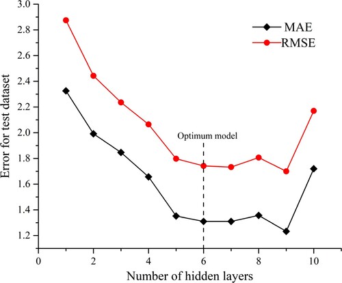
Figure 5. Architecture of the optimum ANN model.

2.2.2. Gaussian process regression

In the past, GPR model has been efficiently used in predicting the response of the system (Gao et al. 2019, Zhang et al. 2019, Suthar 2020). GPR is a kernel-based ML model that is founded on Bayesian theory and statistical learning approach. Such model can be completely defined by the mean and covariance function (kernel) as follows (Rasmussen 2006): (3) $\mu \left(x\right)=\mathrm{E}\left[g\left(x\right)\right]$(3) (4) $K(x,x^{\mathrm{\prime }})=\mathrm{E}\left[\left(g\right(x)-\mu (x\left)\right)\left(g\right(x^{\mathrm{\prime }})-\mu (x^{\mathrm{\prime }}\left)\right)\right]$(4) where $\mu \left(x\right)$is the mean function, and $k(x,x^{\mathrm{\prime }})$is the covariance function of a real process $g\left(x\right)$. The Gaussian process is defined by the set of random parameters, and any finite number of it has the joint Gaussian allocation. Mathematically (Gao et al. 2019): (5) $g\left(x\right)\sim \mathrm{G}\mathrm{P}\left(\mu \right(x),k(x,x^{\mathrm{\prime }}\left)\right)$(5) For detailed derivation, readers are directed to excellent studies available in the literature (Seeger 2004, Rasmussen 2006).

In this study, various kernel functions such as squared exponential, radial bias and Pearson’s VII universal kernel functions are used for estimating the CBR of reinforced soil using GPR. The optimum results are obtained by employing the Pearson’s VII universal kernel (PUK) function. The mathematical form of PUK is given as follows (Üstün et al. 2006): (6) $k(x,x^{\mathrm{\prime }})=1/[1+(2\sqrt{{\parallel x-x^{\mathrm{\prime }}\parallel }^2}\sqrt{2^{\left(1/\omega \right)}-1/\sigma {)}^2}{]}^{\omega }$(6) where $\sigma$and $\omega$are the Person’s width, and peak tailing factor, respectively.

2.2.3. Least median of square regression

The LMSRis a semi-parametric quantile regression technique. In contrary to the classical regression model, the sum of least squares is replaced by the median of squared errors (Rousseeuw 1984). The LMSR overcomes the major drawback in the ordinary regression, that is, the sensitivity to the outliers. For a standard univariate linear regression problem, the residuals take the following form (Massart et al. 1986) (7) $r_j=y_j-a{x}_j-b$(7) where r is the residual, y is the response (output), x is the input, and a and b are regression coefficients. The principle of least square governs, minimise $\sum _{j=1}^n{r}_j^2$, whereas LMS estimators aims at minimising the median of square errors, that is, minimise $\mathrm{m}\mathrm{e}\mathrm{d}\sum _{j=1}^n{r}_j^2$. In this study, the following relationship is obtained for estimating the CBR of reinforced soil by using the LMS regression technique: (8) $\begin{array}{rl}& \mathrm{C}\mathrm{B}{\mathrm{R}}_{\mathrm{L}\mathrm{M}\mathrm{S}\mathrm{R}}=0.0231X_1-0.018X_2+0.1528X_3\\ & -0.015X_5-0.6108X_6+0.0032X_8+\\ & 0.8856X_9-1.3882X_{10}-1.8478X_{11}+57.95\end{array}$(8)

2.2.4. Elastic net regularisation regression

The ENRR is a robust regression model which aims at combining the penalties of the least absolute shrinkage and selection operator (LASSO), $l_1$, and ridge regression technique, $l_2$(Ogutu et al. 2012). LASSO randomly tends to choose only one attribute and ignore the other, especially when the attributes are highly correlated, whereas the elastic net (EN) overcomes this problem. For a set of data sample with n observations and p predictors, let $\left\{\right(x_i,y_i),i=1,2\dots ,n)\}$ , where $x_i,y_i$ belongs to $R^p$. Moreover, if $y=(y_1\dots ,y_n{)}^{\mathrm{T}}$ and $X\in R^{n\times p}$ represents the output vector and model matrix, respectively, then the EN can be written as follows (Zou and Hastie 2005): (9) $\widehat{\text{β}}=\underset{\text{β}}{\arg min}|y-X\text{β}{|}^2,\mathrm{s}\mathrm{u}\mathrm{b}\mathrm{j}\mathrm{e}\mathrm{c}\mathrm{t}\mathrm{e}\mathrm{d}\mathrm{t}\mathrm{o}\xi =(1-\lambda \left)\right|\text{β}{|}_1+\lambda |\text{β}{|}^2\le s\mathrm{f}\mathrm{o}\mathrm{r}\mathrm{s}\mathrm{o}\mathrm{m}\mathrm{e}s$(9) where$\text{β}$is the weight vector, $\xi$ is the EN penalty parameter, that is a combination of $l_1$ and $l_2$. For the detail derivation, readers may refer to the research conducted by Zou and Hastie (2005).

It may be noted that, if $\lambda =1$, then EN takes the ridge regression shape, and if $\lambda =0$, then it takes the LASSO form. For $\lambda \in \left[0,1\right)$, the EN encompasses the characteristics of both the ridge and LASSO. In other words, the penalty parameter $l_1$ enables the automatic selection of variables and $l_2$ leads to stabilisation by making the problem strictly convex (Gao et al. 2019). For the estimation of CBR, the following relationship is obtained through ENRR regression: (10) $\begin{array}{rl}& \mathrm{C}\mathrm{B}{\mathrm{R}}_{\mathrm{E}\mathrm{N}\mathrm{R}\mathrm{R}}=0.229X_1+\mathrm{0..229}{X}_2-0.237X_4-0.421X_5\\ & -0.028X_6+0.261X_7+0.027X_8+\\ & 0.225X_9-0.069X_{10}+0.039X_{11}-1.240\end{array}$(10)

2.2.5. Lazy K-star

Lazy learning is a ML method in which the majority of the computation time is deferred to the consultation time, that is, until a query (call) is made to the system (Webb et al. 2011). LKS is a lazy learning algorithm which performs the generalisation of the training data using instant base learning classification. This means that unlike the ANN or other ML methods, the predictions are not inferred from particular instances in the training data, instead the complete data are stored in the memory and upon call, the response is produced by the nearest neighbour approach. The K-star sums all the possible transitions between the two instances and amalgamate them into a single class (Cleary and Trigg 1995). This is achieved by summing the probabilities over all possible transformations between the instances. This entropy-based learning technique has several advantages in comparison to other rule-based schemes, such as better handling of missing values and common attributes. Mathematically, the function K-star is defined as follows (Cleary and Trigg 1995, Gao et al. 2019): (11) $K^{\ast }=-\log P^{\ast }\left(q\right|p)$(11) where $P^{\ast }$ represents the probability function, that is, the probability of all the paths from instances p to q.

2.2.6. M-5 model trees

Based on the original research conducted by Quinlan (1992) on the development of decision trees for the regression problem, Wang and Witten (1997) proposed the M-5 model. The M-5 model uses the classical top-down method for growing and pruning decision trees. The data are presented in the form of the mean values and regression function to the leaf nodes; thereafter, the branching/separation is performed at each node (MLR) until the values of response variables reaching a node shows no or negligible change. In the next step, the larger subtrees are replaced by a single larger linear model. For this, the error values inside the inner node of the tree end are compared with those of the tree leaf underlying that node (Khorrami et al. 2020). Finally, the smoothing function is applied to trim the gaps between the neighbouring (adjacent) leaf nodes. In this way, the final model is obtained by combining all the available linear models along the path from the root node of the tree to each leaf node; thus, effectively producing a linear combination of all the available linear models (Quinlan 1992, Khorrami et al. 2020).

2.2.7. Alternative model trees

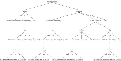
AMT is a recently developed algorithm based on the principle of ensemble learning. Originally, proposed by Frank et al. (2015), AMT uses the additive regression technique to grow the trees. Moreover, similar to the decision trees, AMT utilises stage-wise forward additive regression (statistical boosting variant) and cross-validation technique to minimise the square errors and to limit the growth of the trees, respectively (Moayedi et al. 2020). The main difference between the M-5 model trees and AMT model is that the former uses the multivariate linear regression on the leaves, while the latter employs the simple linear regression to obtain the predictive model. For this, AMT utilises two nodes, namely splitter node and predictor node. The splitter node splits the numeric attributes at the median value, and the predictor node predicts the response of the system by using the linear regression technique (Gao et al. 2019, Moayedi et al. 2020). For detailed insight and derivation, the reader may refer to Frank et al. (2015). AMT model proposed for the present study for estimating the CBR of reinforced soil is illustrated in Figure 6.

Figure 6. AMT model proposed for estimating the CBR of reinforced soil.

2.2.8. Random forest

RF is an ensemble learning method originally suggested by Ho (1995) for classification and regression problems. At its core, the RF works by creating a swarm of decision trees and then averaging the output of each tree. The bootstrap aggregating technique helps the RF to obtain a much stable solution, and reduces the chances of overfitting (Breiman 2001). The user control parameters are the number of trees, number of nodes, and number of variables. Generally, the higher number of trees will lead to higher accuracy but require more computation time. As each tree works entirely independently and uses out-of-bag estimates to observe the errors and correlation strength, the abundance of trees will not lead to overfitting of the model. The detailed algorithm is described in Breiman (2001).

2.3. Model assessment criteria

Five statistical matrices were chosen to appraise and compare the predictive strength of all the developed data-driven models. The matrices are as follows: (i) coefficient of determination (R²); (ii) root means square error (RMSE); (iii) scatter index (SI); (iv) index of agreement (I_a) and (v) mean absolute error (MAE). All these statistical tools have been extensively used in the previous studies to simulate the accuracy of ML-based models (Yaseen et al. 2018, Khorrami et al. 2020, Raja and Shukla 2020, 2021). The mathematical form of these statistical standards is given below (12) $R^2=1-\frac{\sum _{i=1}^n{(\mathrm{C}\mathrm{B}{\mathrm{R}}_{o_i}-\mathrm{C}\mathrm{B}{\mathrm{R}}_{p_i})}^2}{\sum _{i=1}^n{(\mathrm{C}\mathrm{B}{\mathrm{R}}_{o_i}-\overline{\mathrm{C}\mathrm{B}{\mathrm{R}}_o})}^2}$(12) (13) $\mathrm{R}\mathrm{M}\mathrm{S}\mathrm{E}=\sqrt{\frac{1}{n}\sum _{i=1}^n{(\mathrm{C}\mathrm{B}{\mathrm{R}}_{o_i}-\mathrm{C}\mathrm{B}{\mathrm{R}}_{p_i})}^2}$(13) (14) $\mathrm{S}\mathrm{I}=\frac{\sqrt{{\displaystyle \frac{1}{n}\sum _{i=1}^n{(\mathrm{C}\mathrm{B}{\mathrm{R}}_{o_i}-\mathrm{C}\mathrm{B}{\mathrm{R}}_{p_i})}^2}}}{\overline{\mathrm{C}\mathrm{B}{\mathrm{R}}_o}}$(14) (15) $I_a=1-\frac{\sum _{i=1}^n{(\mathrm{C}\mathrm{B}{\mathrm{R}}_{o_i}-\mathrm{C}\mathrm{B}{\mathrm{R}}_{o_p})}^2}{\sum _{}^{}{\left(\left|\mathrm{C}\mathrm{B}{\mathrm{R}}_{o_i}-\overline{\mathrm{C}\mathrm{B}{\mathrm{R}}_o}\right|+\left|\mathrm{C}\mathrm{B}{\mathrm{R}}_{p_i}-\overline{\mathrm{C}\mathrm{B}{\mathrm{R}}_o}\right|\right)}^2}$(15) (16) $\mathrm{M}\mathrm{A}\mathrm{E}=\frac{1}{n}\sum _{i=1}^n\left|\mathrm{C}\mathrm{B}{\mathrm{R}}_{p_i}-\mathrm{C}\mathrm{B}{\mathrm{R}}_{o_i}\right|$(16) where n is the number of observations, $\mathrm{C}\mathrm{B}{\mathrm{R}}_{o_i}$is the ith observed (measured) value, $\mathrm{C}\mathrm{B}{\mathrm{R}}_{p_i}$ is the ith predicted value, $\overline{\mathrm{C}\mathrm{B}{\mathrm{R}}_o}$ is mean observed value, and $\overline{\mathrm{C}\mathrm{B}{\mathrm{R}}_p}$ is the mean predicted value. The range of R² is 0–1 and for an ideal model, the value should be close to 1. The I_a (0 ≤ I_a ≤ 1) shows the ratio of mean square error and the prediction error in the system. The value of 1 represents the perfect agreement between the observed and predicted value and 0 represents no agreement (Willmott 1981). RMSE and MAE are widely adopted for assessing the predictive accuracy of the ML models. The MAE represents the average error (equal weightage) over the data set without considering the sign. It means that in MAE, the difference between the observed and predicted values is averaged in a linear manner, while in RMSE, the errors are squared before taking the average (Equation (13)), therefore giving high weightage to the larger errors (Yaseen et al. 2018). For an ideal model, both MAE and RMSE value should be 0. SI represents the ratio of RMSE to the average of observed values. Lower values of SI depict more accuracy and vice-versa (Khorrami et al. 2020)

3. Results and discussion

As mentioned abovethat the main aim of this study is the comprehensive ML-based analysis for modelling the CBR of GRS. Main parameters of all the models are summarised in Table 4. For evaluating the performance of the developed prescient models, namely ANN, LMSR, GPR, ENRR, K-star, M-5, AMT, and RF, the calculated values of all the statistical parameters, namely R², RMSE, SI, I_a and MAE are presented in Table 5 for testing (validation) data. The colour intensity coding technique (CICT) has been applied to indicate the strength of each parameter according to its obtained value. It may be noted that this technique has been successfully applied in many previous studies (Nazari et al. 2020, Nguyen et al. 2020). In this way, the parameters which illustrate more accuracy (higher R² and I_a; and lower RMSE, SI and MAE) are given intense colour and vice-versa. For this study, the shades of green colour are used for depicting the predictive accuracy of the developed ML models. The dark green colour cells show more accuracy, and light pale green colour cells depict the lower precision level. Accordingly, each model was scored, and the final ranking for a particular model was obtained by summation of all the partial scores given based on the statistical indices’ values.

Table 4: Main parameters of the models

Name	Parameters
ANN	Hidden layers = 1; Hidden nodes = 6; Transfer function = Sigmoid; Learning rate = 0.3; Momentum term = 0.2
GPR	Kernel = PuK; $\omega =1$, σ = 1
LMSR	S = 4, G = 0
ENRR	Alpha = 0.001, lambda-seq-threshold = 1.0E-7, number of iteration folds = 10, epsilon = 0.0004
LKS	Global blending parameter (B) = 20
M-5	Minimum no. of instances at leaf nodes (M) = 4.0
AMT	No. of iterations (I) = 100, shrinkage (H) = 1
RF	No. of iterations (I) = 100, max depth (K) = 0, V = 0.001

Table 5. Results of colour intensity ranking criteria for all the proposed models in predicting the CBR of reinforced soil

As Table 5 reports, the LKS and ANN models have shown superior predictive accuracy in estimating the CBR value of reinforced soil. This can be established from the indicated total scores of 40 and 35, respectively, for LKS and ANN models. The calculated values of the statistical indices for ANN, LMSR, GPR, ENRR, LKS, M-5, AMT and RF, such as R² (0.944, 0.63, 0.939, 0.807, 0.955, 0.847, 0.927 and 0.932), and MAE (1.27, 5.46, 2.02, 2.19, 1.04, 1.8, 1.30 and 1.29), indicate the best correlation and less absolute error between the actual and simulated values of the CBR for these two models (i.e. LKS and ANN). Also, the SI (0.226, 0.91, 0.51, 0.42, 0.213, 0.44, 0.278 and 0.273) and I_a (0.984, 0.74, 0.907, 0.932, 0.987, 0.948, 0.980 and 0.976) further prove this fact. In concurrence with the same argument, the reliability of AMT and RF trees models can also be established. However, the computed values of MAE (5.46, 2.02, 2.19 and 1.8) and RMSE (10.85, 3.37, and 3.22 and 2.91) for LMSR, GPR, ENRR and M-5 respectively, indicate that the forecasting ability of these models are associated with relatively high bias, in comparison to their counterpart models.

The scholars have argued that the reliability of the ML models should also be assessed using the external validation and/or multi-criteria approach (Gandomi et al. 2013, Naser and Alavi 2020). This gives the realistic evaluation of the model’s predictive performance by eradicating/minimising the bias associated with the traditional goodness of fit indices. Therefore, the external model validation criteria by Golbraikh et al. (2003), stabilisation criteria for quantitative structure–activity relationship (QSAR) model by Roy and Roy (2008), and objection function (OBJ) by Gandomi et al. (2013) are also applied to further affirm the accuracy and reliability of the developed data-driven models.

According to Golbraikh et al. (2003), a model must meet the following criteria to be considered reliable. One of the slope regressions lines ($k$ or $k^{\mathrm{\prime }}$) between the observed values (say x_i) and predicted values (y_i) or vice-versa must pass through the origin, and must be close to unity. In terms of the CBR prediction model, it can be written as follows: (17) $k=\frac{{\sum }_{i=1}^n(\mathrm{C}\mathrm{B}{\mathrm{R}}_{o_i}\times \mathrm{C}\mathrm{B}{\mathrm{R}}_{p_i})}{{\mathrm{C}\mathrm{B}\mathrm{R}}_{o_i}^2}$(17) (18) $k^{\mathrm{\prime }}=\frac{{\sum }_{i=1}^n(\mathrm{C}\mathrm{B}{\mathrm{R}}_{o_i}\times \mathrm{C}\mathrm{B}{\mathrm{R}}_{p_i})}{{\mathrm{C}\mathrm{B}\mathrm{R}}_{p_i}^2}$(18) The value of $k$ or $k^{\mathrm{\prime }}$must be between 0.85 and 1.15. Additionally, the performance index parameters, that are, m and n should be <0.1 and can be calculated as follows: (19) $m=\frac{R^2-R_o^2}{R^2}$(19) (20) $n=\frac{R^2-R{\mathrm{\prime }}_o^2}{R^2}$(20) whereas $R_o^2$ and $R{\mathrm{\prime }}_o^2$are the regression coefficients and can be estimated as (21) $R_o^2=1-\frac{\sum _{i=1}^n{\mathrm{C}\mathrm{B}\mathrm{R}}_{o_i}^2{\left(1-k\right)}^2}{\sum _{i=1}^n{\left(\mathrm{C}\mathrm{B}{\mathrm{R}}_{p_i}-\overline{\mathrm{C}\mathrm{B}{\mathrm{R}}_o}\right)}^2}$(21) (22) $R{\mathrm{\prime }}_o^2=1-\frac{\sum _{i=1}^n{\mathrm{C}\mathrm{B}\mathrm{R}}_{p_i}^2{\left(1-k\mathrm{\prime }\right)}^2}{\sum _{i=1}^n{\left(\mathrm{C}\mathrm{B}{\mathrm{R}}_{p_i}-\overline{\mathrm{C}\mathrm{B}{\mathrm{R}}_p}\right)}^2}$(22) Ideally, the values of $R_o^2$or $R{\mathrm{\prime }}_o^2$ should be close to actual $R^2$, whereas $R^2$ should be > 0.6. In this way, the model is considered acceptable if it meets all these criteria.

Roy and Roy (2008) established the stabilisation criteria for ensuring the predictability of the developed model. Accordingly, the value of $R_m$ is estimated as stabilisation criterion to measure the reliability of the developed model. Mathematically (23) $R_m=R^2\times \left(1-\sqrt{\left|R^2-R_o^2\right|}\right)$(23) The value of $R_m$ should be > 0.5.

Based on RMSE, R² and MAE, the OBJ function contemplates the performance of the model is training and testing data set, simultaneously (Gandomi et al. 2013). The smaller the function value, the better it is and vice-versa. Mathematically (24) $\mathrm{O}\mathrm{B}\mathrm{J}=\left(\frac{\mathrm{N}\mathrm{o}{.}_{\mathrm{t}\mathrm{r}}\text{-}\mathrm{N}\mathrm{o}{.}_{\mathrm{t}\mathrm{s}}}{\mathrm{N}\mathrm{o}{.}_{\mathrm{t}\mathrm{r}}+\mathrm{N}\mathrm{o}{.}_{\mathrm{t}\mathrm{s}}}\right)\times \frac{\mathrm{R}\mathrm{M}\mathrm{S}{\mathrm{E}}_{\mathrm{t}\mathrm{r}}+\mathrm{M}\mathrm{A}{\mathrm{E}}_{\mathrm{t}\mathrm{r}}}{R_{\mathrm{t}\mathrm{r}}^2+1}+\left(\frac{2\mathrm{N}\mathrm{o}{.}_{\mathrm{t}\mathrm{s}}}{\mathrm{N}\mathrm{o}{.}_{\mathrm{t}\mathrm{r}}+\mathrm{N}\mathrm{o}{.}_{\mathrm{t}\mathrm{s}}}\right)\times \frac{\mathrm{R}\mathrm{M}\mathrm{S}{\mathrm{E}}_{\mathrm{t}\mathrm{s}}+\mathrm{M}\mathrm{A}{\mathrm{E}}_{\mathrm{t}\mathrm{s}}}{R_{\mathrm{t}\mathrm{r}}^2+1}$(24) where subscripts tr and ts represent training and testing data, respectively.

The results of the above-mentioned external validation and multi-criteria approach are summarised in Table 6. From the table, it can be concurred that the ANN, LKS, AMT and RF models have shown excellent prediction ability in calculating the CBR of reinforced soil. This is substantiated by the fact that all these models have met the underlying conditions corresponding to the external validation criteria approach. The ENRR and M-5 models have met all the conditions of Golbraikh et al. (2003) model but failed to meet the model stabilisation condition with R_m values of 0.27 and 0.37, respectively. Based on the values of OBJ function values (3.40, 15.43, 5.38, 5.44, 2.95, 4.79, 3.52 and 3.56), respectively, for ANN, LMS, GPR, ENRR, LKS, M-5 trees, AMT and RF also indicate that the ANN and LKS can be established as the best models for predicting the CBR of reinforced soil. Also, the AMT and RF models performed well by meeting all the criteria, and therefore can be introduced as third- and fourth-best models in the hierarchy. This means that the predictions made by these models are trustworthy and are not a mere coincidence. Additionally, the results of LMS, GPR, ENRR and M-5 models indicate relatively poor performance in comparison to their counterpart models.

Table 6. Results of external validation and multi-criteria approach used for accessing the accuracy of all the developed ML models

Parameters for accessing the accuracy with respect to external model validation criteria						External validation criteria			Stabilisation criteria for QSAR model		Objective function
						Golbraikh et al. (2003)			Roy and Roy (2008)		Gandomi et al. (2013)
ML models	$R^2$	$k$	$k^{\mathrm{\prime }}$	m	n	Condition 1	Condition 2	Condition 3	Rm	Rm >0.5	OBJ
ANN	0.944	0.975	0.997	−0.12	−0.12	✓	✓	✓	0.60	✓	3.40
LMSR	0.630	0.479	1.635	0.24	0.92	✓	x	x	0.27	x	15.43
GPR	0.939	1.262	0.736	0.37	0.17	✓	✓	x	0.38	x	5.38
ENRR	0.807	1.022	0.880	−0.53	−0.45	✓	✓	✓	0.27	x	5.44
LKS	0.955	1.026	0.953	−0.09	−0.09	✓	✓	✓	0.65	✓	2.95
M-5	0.847	1.104	0.839	−0.33	−0.25	✓	✓	✓	0.37	x	4.79
AMT	0.927	1.007	0.957	−0.16	−0.15	✓	✓	✓	0.54	✓	3.52
RF	0.932	1.039	0.925	−0.14	−0.13	✓	✓	✓	0.56	✓	3.56

Note: Conditions 1, 2 and 3 correspond to$R^2\ge 0.6$; $0.85\le k\le 1.15$ or $0.85\le k^{\mathrm{\prime }}\le 1.15$; and m, n < 0.1, respectively.

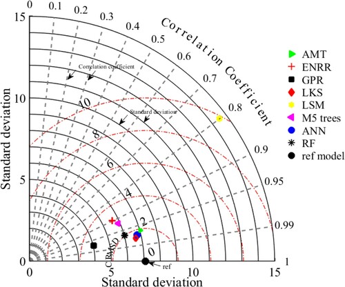
Finally, Taylor’s diagram originally proposed by Taylor (2001) has been presented in Figure 7. The Taylor diagram presents the visual summary of the predictive power of the data-driven models on a single platform, that is, how closely the actual and simulated responses are related to each other in terms of their correlation and biasness ratio (Taylor 2001, Raja and Shukla 2020). Regarding Figure 7, the solid radial lines (black) represent the standard deviation (SD); thickened dash lines (grey) represent the correlation coefficient (CC); and the dotted radial lines (red) show the centred root mean square deviation (CRMSD) between the simulated (test data) and reference field. The reference model is indicated by the solid black dot with the measured SD of 7.09, CC of unity and zero CRMSD. It can be observed that for LKS and ANN models, the CC, CRMSD and SD are about (0.977, 1.53 and 6.64) and (0.9716, 1.68 and 6.76), respectively. This highlights excellent predictive capability for the developed models followed by AMT model with values of CC, CRMSD and SD of 0.963, 1.92 and 7.02, respectively. For the same parameters, the values for M-5 and RF were (0.921, 2.83 and 5.89) and (0.965, 1.99 and 6.02), respectively. On the contrary, the GPR model has shown little too spatial variability with the SD value of ∼4.03, and the LSM model has depicted a large variation in comparison to the observed CBR values with the SD of 14.59. The ENRR model has shown a fair overall performance with the SD value of 5.76; however, the correlation is weak (CC = 0.897), and root mean square error is high (CRMSD = 3.21). Therefore, consistent with the results of the statistical indices and external validation criteria, to this point, it can be established with sufficient trustworthiness, that among all the applied ML models, ANN and LKS models have achieved more accuracy in forecasting the CBR of reinforced soil.

Figure 7. Taylor diagram presenting the visual summary of predictive strength of developed models.

4. Model presentation

For this work, ANN is selected as an appropriate estimator of the CBR values of the GRS, due to its predictive performance and simplicity. The ANN-based equation is given as follows (Aamir et al. 2020): (25) $y=g_n\left(\sum _{j=1}^h{w}_{jk}{f}_n\left({\theta }_j+\sum _i^n{\text{β}}_{ji}{X}_i\right)+{\theta }_k\right)$(25) where y is the value of output (CBR), g_n is the hidden–output layer transfer function (pureline), f_n is the input-hidden layer transfer function (sigmoid), w_jk is the weight connection between the jth node in the hidden layer and single node in the output layer (k = 1), ${\text{β}}_{ji}$ is the weight connection between the ith node of the input layer and jth node of the hidden layer, ${\theta }_j$ is the bias of the jth node at the hidden layer and ${\theta }_k$ is the bias at the output layer node. The architecture of the developed single hidden layer neural network is already given in Figure 5, that is, 11 input nodes, 6 hidden nodes and 1 output node. The weights and biases values of the network are reported in Table 7. The values of input parameters should be normalised [−1,1] before feeding to ANN using the following relationship (26) $X^{\mathrm{\prime }}=2\frac{X-X_{min}}{X_{max}-X_{min}}-1$(26) where X_min is the minimum value of the parameter, and X_max is the maximum value of the parameter, and already given in Table 1.

Table 7. Weights and biases of the developed neural network

Weights of input layer – hidden layer, ${\text{β}}_{ij}$											Hidden layer bias ${\theta }_j$
1	2	3	4	5	6	7	8	9	10	11
−0.2536	−0.4607	−0.0521	−0.04	0.2659	−0.2427	−0.4646	1.1754	0.6772	−1.103	0.4061	−0.9167
−0.2914	−0.3918	−0.1618	−0.0108	0.6409	−0.3343	0.0960	0.4698	0.3662	0.3322	0.3849	−0.7143
−0.12738	−0.0038	−0.3035	0.4085	0.6231	−0.3620	0.0739	0.8576	0.4965	0.7954	0.5570	−0.5705
−0.8386	−1.806	0.2339	−0.0798	−1.819	−0.0626	1.2337	1.6369	0.4646	−0.6744	0.4908	−1.1191
−1.4253	−1.7292	−1.0318	1.2547	0.7067	1.8706	−2.8545	−0.7062	−1.0057	0.5092	−0.1882	1.1229
−0.7382	−1.3429	−0.1035	−0.1969	1.1933	−0.9824	0.5970	−0.7195	−0.8305	−0.0584	−0.4887	−0.3609
Weights of hiden-ouput layer, $w_{jk}$											Output layer bias ${\theta }_k$
−1.022	−0.322	−0.8921	1.4719	−2.087	−1.234						1.6104

In order to estimate the CBR of reinforced soil with 11 input parameters, the following relationship is established for the optimum ANN model (27) $\mathrm{C}\mathrm{B}{{\mathrm{R}}^{\mathrm{\prime }}}_p=\sum _{j=1}^{11}{w}_{jk}\mathrm{s}\mathrm{i}\mathrm{g}{\left(\alpha \right)}_j+{\theta }_k$(27) (28) ${\alpha }_j={\text{β}}_{1j}{X}_1^{\mathrm{\prime }}+{\text{β}}_{2j}{X}_2^{\mathrm{\prime }}+{\text{β}}_{3j}{X}_3^{\mathrm{\prime }}+{\text{β}}_{4j}{X}_4^{\mathrm{\prime }}+{\text{β}}_{5j}{X}_5^{\mathrm{\prime }}+{\text{β}}_{6j}{X}_6^{\mathrm{\prime }}+{\text{β}}_{7j}{X}_7^{\mathrm{\prime }}+{\text{β}}_{8j}{X}_8^{\mathrm{\prime }}+{\text{β}}_{9j}{X}_9^{\mathrm{\prime }}+{\text{β}}_{10j}{X}_{10}^{\mathrm{\prime }}+{\text{β}}_{11j}{X}_{11}^{\mathrm{\prime }}+{\theta }_j$(28) where $\mathrm{C}\mathrm{B}{{\mathrm{R}}^{\mathrm{\prime }}}_p$ is the normalised predicted CBR value [−1,1]; $X_1^{\mathrm{\prime }},X_2^{\mathrm{\prime }},X_3^{\mathrm{\prime }},X_4^{\mathrm{\prime }},X_5^{\mathrm{\prime }},X_6^{\mathrm{\prime }},X_7^{\mathrm{\prime }},X_8^{\mathrm{\prime }},X_9^{\mathrm{\prime }},X_{10}^{\mathrm{\prime }}$and $X_{11}^{\mathrm{\prime }}$ represents the normalised values of all the input parameters. The predicted CBR value should be de-normalised as follows: (29) $CBR=(CB{R}_p^{\mathrm{\prime }}+1)\times (CB{R}_{max}-CB{R}_{min})/2+CB{R}_{min}$(29) For easy comprehension, the design example is given in the Appendix. It may be noted that the present relation is only calibrated and validated for predicting the soaked CBR of GRSs within the training data range, and therefore, shall not be used for estimating the unsoaked CBR values, and the CBR of unreinforced soil or soil reinforced with other types of reinforcements such as fibres, tire chips, metals, etc.

4.2. Independent validation

LKS and ANN models have shown excellent predictive performance for the data set utilised to establish the ML models. However, in order to establish the supremacy, consistency and reliability of any ML model, its predictive strength should be checked against the entirely new data. Therefore, an experimental study was conducted to establish a new data set. For this, six soaked CBR tests (see Table 3) were conducted and their experimental values were compared with the simulated values obtained from ANN and LKS models.

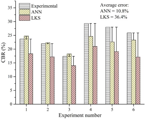
The vis-à-vis comparison of the experimental and predicted CBR values for ANN and LKS is presented in Figure 8. It can be observed that the ANN predicted the CBR values much closer to the actual values in comparison to LKS with the average absolute error of 10.8% and 36.4%, respectively. Therefore, it is admissible that the ANN model has outperformed its competitive models in predicting the CBR of GRS. Moreover, another main advantage of the ANN network in comparison to other efficient models (say LKS or AMT) is that it can be translated into a trackable functional relationship, and, therefore, can easily be executed without the need for any expensive computer-based program. Moreover, the ANN model can be updated to acquire the better results by presenting more training examples when the new data becomes available.

Figure 8. Comparison of the experimental and predicted CBR values for ANN and LKS models.

5. Sensitivity analysis

A sensitivity analysis has also been carried out to determine the relative importance of each parameter affecting the CBR of reinforced soil. It helps in finding the strength of the existing correlation between the input and output dimensions. For this study, the cosine amplitude method (CAM) is used to establish the strength of input parameters with the CBR of reinforced soil.

For CAM, let n data samples in the same region (say X-space), then the data array X can be written as follows (Hasanzadehshooiili et al. 2012): (30) $X=\{x_1,x_2,x_3\dots ,x_m\}$(30) Each element$x_i$ of data array X is the vector (length m) in Equation (30), and is defined as: (31) $x_i=\{x_{i1},x_{i2},x_{i3}\dots ,x_{im}\}$(31) In this way, the correlation strength $r_{ij}$ between the data points $x_i$and$x_j$can be estimated by Equation (32) (Ghorbani et al. 2020c) (32) $r_{ij}=\frac{\sum _{k=1}^m{x}_{ik}{x}_{jk}}{\sqrt{\sum _{k=1}^m{x}_{ik}^2\sum _{k=1}^m{x}_{jk}^2}},0\le r_{ij}\le 1$(32) The result of the CAM sensitivity analysis carried for the ANN model is illustrated in Figure 9. The relative strengths of all the input parameters ($X_1,X_2,X_3,X_4,X_5,X_6,X_7,X_8,X_9,X_{10}$and$X_{11}$) with CBR of reinforced soil are 0.761, 0.756, 0.759, 0.721, 0.766, 0.731, 0.40, 0.560, 0.676, 0.761 and 0.30, respectively. 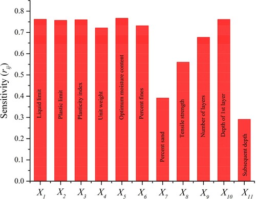This imply that all the input parameters except for the subsequent reinforcement depth (X₁₁) play a significant role in determining the CBR of reinforced soil with $r_{ij}$ approximately ranging from 0.4 to 0.8. Moreover, X₁ (LL), X₅ (OMC) and depth of the first reinforcement layer (X₁₀) has achieved the highest correlation in predicting the CBR of reinforced soil.

Figure 9. CAM sensitivity analysis for the developed ANN model.

6. Conclusions and future outlook

This work presents the comprehensive and detailed comparison of eight data-driven ML-based models, namely ANN, LMSR, GPR, ENRR, LKS, M-5 model trees, AMT and RF for predicting the CBR of subgrade soil reinforced with geosynthetic layers. For this, the pertinent data set was retrieved from previously published scientific studies. Each sample consisted of 11 input variables such as LL, PL, PI, maximum dry unit weight of soil, moisture content, percentage fines, percentage sand, tensile strength of geosynthetic reinforcement, number of reinforcement layers, position of the first reinforcement layer and position of the subsequent reinforcement layers, and one output variable, that is, CBR. The acquired data set was randomly divided into training (i.e. 60% of total data) and 40% testing (i.e. 40% of total data) to calibrate and validate the performance of all the data-driven tools. The performance of all the models was accessed using the five statistical indices, which are, coefficient of determination (R²), root means square error (RMSE), scatter index (SI), index of agreement (I_a) and mean absolute error (MAE). Based on the results of these indices, a colour intensity coded ranking model was developed. Moreover, the predictive strength of the tools mentioned supra was also appraised using the external validation criteria and multi-criteria approach. The most appropriate models were also tested against the entirely independent validation data obtained by conducting the new CBR tests. Finally, the sensitivity analysis was performed to assess the effect of the input parameters on the CBR value. Based on the acquired results, the following conclusions can be drawn.

• In the CBR approximation, the values of R² (0.944, 0.63, 0.939, 0.807, 0.955, 0.847, 0.927 and 0.932), RMSE (1.74, 10.85, 3.37, 3.22, 1.52, 2.91, 1.94 and 2.03), SI (0.226, 0.91, 0.51, 0.42, 0.213, 0.44, 0.278 and 0.273), I_a (0.984, 0.74, 0.907, 0.932, 0.987, 0.948, 0.98 and 0.976), and MAE (1.27, 5.46, 2.02, 2.19, 1.04, 1.80, 1.30 and 1.29) were, respectively, calculated for ANN, LMSR, GPR, ENRR, LKS, M-5 trees, AMT and RF models. Based on the values of these statistical indices, a total ranking score was obtained for all the modelling techniques. The results have shown excellent prediction ability of LKS and ANN with a total score of 40 and 35, respectively. The ranking scores of other models such as LMSR, GPR, ENRR, M-5 trees, AMT and RF were, respectively, 5, 15, 14, 18, 26 and 27.

• Among all the models, the LMSR model has obtained the poorest approximation of the CBR and its insufficiency was depicted by the ranking score (total score = 5) obtained based on the above-mentioned assessment criteria.

• Based on the results of the external validation technique, and multi-criteria assessment approach, the ANN, LKS, AMT and RF models have achieved good prediction ability and model stability in forecasting the CBR of reinforced soil. However, the LKS and ANN have shown superior performance in comparison to their counterpart models with the OBJ function value of 2.95 and 3.40, respectively. Also, among these two models, the latter has predicted the new experimental data (independent data) with more accuracy. Additionally, for this work, the developed ANN model was also converted into trackable mathematical relationship for easy hand or spreadsheet calculations.

• The strength (r_ij) of each input variable with respect to the output (CBR) was evaluated by sensitivity analysis. The results revealed that all the parameters have played an important role in determining the CBR of reinforced soil. However, OMC LL and position of the first reinforcement layer with r_ij values of 0.77, 0.762 and 0.761, respectively, are the most influential parameters.

In this study, to maximise the modelling efficiency and ease of use, default settings are used in WEKA for most of the individual models. Therefore, future studies should focus on how the parameters in the models can be optimised automatically. This limitation can be explored in future by combining some optimisation scheme with the model network. Most recently, the use of evolutionary algorithm based on metaheuristics (e.g. shuffled frog algorithm, grey wolf optimiser, ant lion optimiser, elephant herd optimisation, etc.) has shown good ability to improve the prediction ability of neural networks by optimising its weights and biases. The future work with the focus on such optimisation techniques can prove to be a useful idea. Moreover, the ensemble learning techniques in which the learning power of the multiple ML models are combined to predict the response of the system might also be applied in the future.

Disclosure statement

No potential conflict of interest was reported by the author(s).

Additional information

Funding

The authors would like to thank Edith Cowan University (ECU), Australia and Higher Education Commision, Pakistan, for supporting this research jointly.

Appendix. Design numerical example

Find the CBR of a geosynthetic-reinforced subgrade soil with the following characteristics:

LL (X₁) = 35, plastic limit (X₂) = 25, PI (X₃) = 10, dry unit weight of soil (X₄) = 18.3 kN/m³, moisture content (X₅) = 11.9, percentage fines (X₆) = 67%, percentage sand (X₇) = 32%, tensile strength of geosynthetic reinforcement (X₈) = 35.1 kN/m, number of reinforcement layers (X₉) = 2, position of the first reinforcement layer (X₁₀) = 0.4 and position of subsequent reinforcement layers (X₁₁) = 0.2.

Solution:

Step 1:

Normalise each input using Equation (26): $\begin{array}{rl}& {X^{\mathrm{\prime }}}_1,{X^{\mathrm{\prime }}}_2,{X^{\mathrm{\prime }}}_3,{X^{\mathrm{\prime }}}_4,{X^{\mathrm{\prime }}}_5,{X^{\mathrm{\prime }}}_6,{X^{\mathrm{\prime }}}_7,{X^{\mathrm{\prime }}}_8,{X^{\mathrm{\prime }}}_9,{X^{\mathrm{\prime }}}_{10},{X^{\mathrm{\prime }}}_{11}\\ & =\{-0.01408,0.2821,-0.375,0.3964,-0.7238,0.2124,\\ & -0.2195,0.6487,-0.333,-0.2647,-0.3939\}\end{array}$Step 2:

Estimate normalised CBR utilising Equation (27): $\mathrm{C}\mathrm{B}{{\mathrm{R}}^{\mathrm{\prime }}}_p=\sum _{j=1}^{11}{w}_{jk}\mathrm{s}\mathrm{i}\mathrm{g}{\left(\alpha \right)}_j+{\theta }_k$

Compute ${\alpha }_j$from Equation (28). It may be noted that weights and biases values are given in Table 7. $\begin{array}{rl}& {\alpha }_1=(-0.2536\times -0.01408)+(-0.4607\times 0.2821)\\ & +(-0.0521\times -0.375)+(-0.04\times 0.3964)+(0.2659\times -0.7238)\\ & +(-0.2427\times 0.2124)+(-0.4646\times -0.2195)+(1.1754\times 0.6487)\\ & +(0.6772\times -0.333)+(-1.103\times -0.2647)\\ & +(0.4061\times -0.3939)-0.9167\end{array}$ ${\alpha }_1=-0.5126$Similarly $\{{\alpha }_2,{\alpha }_3,{\alpha }_4,{\alpha }_5,{\alpha }_6\}=\{-1.377,-0.8773,0.1887,1.868,-1.953\}$ $\begin{array}{rl}\mathrm{C}\mathrm{B}{{\mathrm{R}}^{\mathrm{\prime }}}_p& =\sum _{j=1}^{11}(-1.022\times \frac{1}{1+{\mathrm{e}}^{-(-0.5126)}}+\dots ,-1.234\\ & \times \frac{1}{1+{\mathrm{e}}^{-(-1.9537)}})+1.6104=-0.2551\end{array}$Step 3:

De-normalise using Equation (29): $\mathrm{C}\mathrm{B}\mathrm{R}=(-0.2551+1)\times (34-1.3)/2+1.3=13.47\text{\%}$

References

- Aamir, M., et al., 2020. Performance analysis of multi-spindle drilling of Al2024 with TiN and TiCN coated drills using experimental and artificial neural networks technique. Applied Sciences (Switzerland), 10 (23), 1–20.
- Abu-Farsakh, M., et al., 2016. Performance of geosynthetic reinforced/stabilized paved roads built over soft soil under cyclic plate loads. Geotextiles and Geomembranes, 44 (6), 845–853.
- Alawi, M.H., and Rajab, M.I, 2013. Prediction of California bearing ratio of subbase layer using multiple linear regression models. Road Materials and Pavement Design, 14 (1), 211–219.
- Arulrajah, A., et al., 2013. Resilient moduli response of recycled construction and demolition materials in pavement subbase applications. Journal of Materials in Civil Engineering, 25 (12), 1920–1928.
- AS 1289.6.1.1, 2014. Methods of testing soils for engineering purposes Soil strength and consolidation tests – Determination of the California Bearing Ratio of a soil – Standard laboratory method for a remoulded specimen.
- ASTM, D., 2016. Standard test method for California bearing ratio (CBR) of laboratory-compacted. West Conshohocken, PA: ASTM International, 1–9.
- Bishop, Christopher, 2006. Pattern Recognition and machine learning. New York: Springer-Verlag New York.
- Breiman, L, 2001. Random forests. Machine Learning, 45 (1), 5–32.
- Carlos, D.M., Pinho-Lopes, M., and Lopes, M.L, 2016. Effect of geosynthetic reinforcement inclusion on the strength parameters and bearing ratio of a fine soil. Procedia Engineering, 143, 34–41.
- Chen, Q., et al., 2018. Performance evaluation of full-scale geosynthetic reinforced flexible pavement. Geosynthetics International, 25 (1), 26–36.
- Choudhary, A., et al., 2012. Improvement in CBR of the expansive soil subgrades with a single reinforcement layer. Proceedings of Indian Geotechnical Conference, 289–292.
- Choudhary, A.K., Jha, J.N., and Gill, K.S., 2011. Improvement in CBR values of expansive soil-subgrades using geosynthetics. Punjab: Guru Nanak Dev Engineering College Ludhiana, 155.
- Cleary, J.G., and Trigg, L.E, 1995. K*: an instance-based learner using an entropic distance measure. Machine Learning Proceedings, 1995, 108–114.
- Cuelho, E. V., Perkins, S.W., and Ganeshan, S.K., 2005. Determining geosynthetic material properties pertinent to reinforced pavement design. Geotechnical Special Publication, 130–142, 241–252.
- Daneshvar, D. and Behnood, A, 2020. Estimation of the dynamic modulus of asphalt concretes using random forests algorithm. International Journal of Pavement Engineering.1-11. https://doi.org/10.1080/10298436.2020.1741587
- de Souza, W.M., Ribeiro, A.J.A., and da Silva, C.A.U., 2020. Use of ANN and visual-manual classification for prediction of soil properties for paving purposes. International Journal of Pavement Engineering.1- 9. https://doi.org/10.1080/10298436.2020.1807546
- Duncan-Williams, E., and Attoh-Okine, N.O, 2008. Effect of geogrid in granular base strength – An experimental investigation. Construction and Building Materials, 22 (11), 2180–2184.
- Erzin, Y., and Turkoz, D, 2016. Use of neural networks for the prediction of the CBR value of some Aegean sands. Neural Computing and Applications, 27 (5), 1415–1426.
- Frank, E., Mayo, M., and Kramer, S., 2015. Alternating model trees. In: Proceedings of the ACM Symposium on Applied Computing, 871–878.
- Gandomi, A.H., Yun, G.J., and Alavi, A.H, 2013. An evolutionary approach for modeling of shear strength of RC deep beams. Materials and Structures/Materiaux et Constructions, 46 (12), 2109–2119.
- Gao, W., et al., 2019. Comprehensive preference learning and feature validity for designing energy-efficient residential buildings using machine learning paradigms. Applied Soft Computing Journal, 84. https://doi.org/10.1016/j.asoc.2019.105748
- Ghorbani, B., et al., 2020a. Experimental investigation and modelling the deformation properties of demolition wastes subjected to freeze–thaw cycles using ANN and SVR. Construction and Building Materials, 258. https://doi.org/10.1016/j.conbuildmat.2020.119688
- Ghorbani, B., et al., 2020b. Experimental and ANN analysis of temperature effects on the permanent deformation properties of demolition wastes. Transportation Geotechnics, 24. https://doi.org/10.1016/j.trgeo.2020.100365
- Ghorbani, B., et al., 2020c. Development of genetic-based models for predicting the resilient modulus of cohesive pavement subgrade soils. Soils Found, 60, 398–412. doi:10.1016/j.sandf.2020.02.010.
- Ghorbani, B., et al., 2021. Shakedown analysis of PET blends with demolition waste as pavement base/subbase materials using experimental and neural network methods. Transportation Geotechnics, 27. https://doi.org/10.1016/j.trgeo.2020.100481
- Ghosh Mondal, P. and Kuna, K., 2020. An automated technique for characterising foamed bitumen using ultrasonic sensor system. International Journal of Pavement Engineering. https://doi.org/10.1080/10298436.2020.1849689
- Golbraikh, A., et al., 2003. Rational selection of training and test sets for the development of validated QSAR models. Journal of Computer-Aided Molecular Design, 17 (2–4), 241–253.
- González Farias, I., Araujo, W., and Ruiz, G., 2018. Prediction of California bearing ratio from index properties of soils using parametric and non-parametric models. Geotechnical and Geological Engineering, 36 (6), 3485–3498.
- Han, C., et al., 2020. Intelligent decision model of road maintenance based on improved weight random forest algorithm. International Journal of Pavement Engineering. https://doi.org/10.1080/10298436.2020.1784418
- Han, J., and Moraga, C, 1995. The influence of the sigmoid function parameters on the speed of backpropagation learning. Lecture Notes in Computer Science (Including Subseries Lecture Notes in Artificial Intelligence and Lecture Notes in Bioinformatics), 930, 195–201.
- Hasanzadehshooiili, H., Lakirouhani, A., and Medzvieckas, J, 2012. Superiority of artificial neural networks over statistical methods in prediction of the optimal length of rock bolts. Journal of Civil Engineering and Management, 18 (5), 655–661.
- Ho, T.K, 1995. Random decision forests. In: Proceedings of the International Conference on Document Analysis and Recognition, ICDAR, 278–282.
- Khorrami, R., Derakhshani, A., and Moayedi, H, 2020. New explicit formulation for shallow foundations’ ultimate bearing capacity rested on granular soil using M-5’ model tree. Measurement, 108032.
- Kuity, A., and Roy, T.K, 2013. Utilization of geogrid mesh for improving the soft subgrade layer with waste material mix compositions. Procedia – Social and Behavioral Sciences, 104, 255–263.
- Massart, D.L., et al., 1986. Least median of squares: a robust method for outlier and model error detection in regression and calibration. Analytica Chimica Acta, 187 (C), 171–179.
- Mittal, A., and Shukla, S, 2018. Influence of geotextile and geogrid reinforcement on strength behaviour of soft silty soil. Applied Mechanics and Materials, 877, 264–269.
- Mittal, A., and Shukla, S, 2019. Strength improvement of poor subgrade soil reinforced with polyester biaxial geogrid. Jordan Journal of Civil Engineering, 13 (2), 214–225.
- Miura, N., et al., 1990. Polymer grid reinforced pavement on soft clay grounds. Geotextiles and Geomembranes, 9 (1), 99–123.
- Moayedi, H., et al., 2020. Feature validity during machine learning paradigms for predicting biodiesel purity. Fuel, 262. https://doi.org/10.1016/j.fuel.2019.116498
- Moayedi, H., and Hayati, S, 2018. Applicability of a CPT-based neural network solution in predicting load-settlement responses of bored pile. International Journal of Geomechanics, 18 (6), 06018009.
- Naeini, S.A., and Ziaie-Moayed, R, 2009. Effect of plasticity index and reinforcement on the CBR value of soft clay. International Journal of Civil Engineering, 7 (2), 124–130.
- Nagaraju, T.V., Prasad, C.D., and Raju, M.J, 2020. Prediction of California bearing ratio using particle swarm optimization. Advances in Intelligent Systems and Computing, 1048, 795–803.
- Nair, A.M., and Latha, G.M, 2011. Bearing resistance of reinforced soil-aggregate systems. Proceedings of the Institution of Civil Engineers: Ground Improvement, 164 (2), 83–95.
- Naser, M., and Alavi, A., 2020. Insights into performance fitness and error metrics for machine learning, 25.
- Nazari, S., et al., 2020. A proper model to predict energy efficiency, exergy efficiency, and water productivity of a solar still via optimized neural network. Journal of Cleaner Production, 277. https://doi.org/10.1016/j.jclepro.2020.123232
- Nazemi, M., and Heidaripanah, A, 2016. Support vector machine to predict the indirect tensile strength of foamed bitumen-stabilised base course materials. Road Materials and Pavement Design, 17 (3), 768–778.
- Negi, M.S. and Singh, S.K, 2019. Experimental and numerical studies on geotextile reinforced subgrade soil. International Journal of Geotechnical Engineering. 1-12. https://doi.org/10.1080/19386362.2019.1684654
- Nguyen, H., et al., 2020. Optimizing ANN models with PSO for predicting short building seismic response. Engineering with Computers, 36 (3), 823–837.
- Ogutu, J.O., Schulz-Streeck, T., and Piepho, H.P, 2012. Genomic selection using regularized linear regression models: ridge regression, lasso, elastic net and their extensions. BMC Proceedings, 6 (Suppl. 2). No. 2, pp. 1-6
- Olowosulu, A.T., et al., 2020. Investigating surface condition classification of flexible road pavement using data mining techniques. International Journal of Pavement Engineering. 1-12. https://doi.org/10.1080/10298436.2020.1847285
- Oztoprak, S., and Bolton, M.D, 2013. Stiffness of sands through a laboratory test database. Geotechnique, 63 (1), 54–70.
- Perkins, S.W, 1999. Mechanical response of geosynthetic-reinforced flexible pavements. Geosynthetics International, 6 (5), 347–382.
- Quinlan, J.R., 1992. Learning with continuous classes. In: Australian Joint Conference on Artificial Intelligence, 343–348.
- Raja, M.N.A. and Shukla, S.K, 2020. An extreme learning machine model for geosynthetic-reinforced sandy soil foundations. Proceedings of the Institution of Civil Engineers – Geotechnical Engineering, 1–42. https://doi.org/10.1680/jgeen.19.00297
- Raja, M.N.A. and Shukla, S.K, 2021. Multivariate adaptive regression splines model for reinforced soil foundations. Geosynthetics International, 1–23. https://doi.org/10.1680/jgein.20.00049
- Rajesh, U., Sajja, S., and Chakravarthi, V.K, 2016. Studies on engineering performance of geogrid reinforced soft subgrade. Transportation Research Procedia, 17, 164–173.
- Rasmussen, C.E., 2006. Gaussian Processes in machine learning. Lecture Notes in Computer Science (including subseries Lecture Notes in Artificial Intelligence and Lecture Notes in Bioinformatics).
- Rousseeuw, P.J, 1984. Least median of squares regression. Journal of the American Statistical Association, 79 (388), 871–880.
- Roy, P.P., and Roy, K, 2008. On some aspects of variable selection for partial least squares regression models. QSAR and Combinatorial Science, 27 (3), 302–313.
- Seeger, M, 2004. Gaussian processes for machine learning. International Journal of Neural Systems, 14 (2), 69–106.
- Shukla, S.K, 2002. Geosynthetics and their Applications. Geosynthetics and their Applications. Thomas Telford.
- Singh, M., Trivedi, A., and Shukla, S.K, 2019. Strength enhancement of the subgrade soil of unpaved road with geosynthetic reinforcement layers. Transportation Geotechnics, 19, 54–60.
- Singh, M., Trivedi, A., and Shukla, S.K., 2020. Fuzzy-based model for predicting strength of geogrid-reinforced subgrade soil with optimal depth of geogrid reinforcement. Transportation Infrastructure Geotechnology.
- Soleimanbeigi, A., and Hataf, N, 2006. Prediction of settlement of shallow foundations on reinforced soils using neural networks. Geosynthetics International, 13 (5), 218–218.
- Suthar, M, 2020. Applying several machine learning approaches for prediction of unconfined compressive strength of stabilized pond ashes. Neural Computing and Applications, 32 (13), 9019–9028.
- Taskiran, T, 2010. Prediction of California bearing ratio (CBR) of fine grained soils by AI methods. Advances in Engineering Software, 41 (6), 886–892.
- Taylor, K.E, 2001. Summarizing multiple aspects of model performance in a single diagram. Journal of Geophysical Research Atmospheres, 106 (D7), 7183–7192.
- Tenpe, A.R., and Patel, A, 2020. Utilization of support vector models and gene expression programming for soil strength modeling. Arabian Journal for Science and Engineering, 45 (5), 4301–4319.
- Ullah, S., Tanyu, B.F., and Zainab, B, 2020. Development of an artificial neural network (ANN)-based model to predict permanent deformation of base course containing reclaimed asphalt pavement (RAP). Road Materials and Pavement Design, 1–19.
- Üstün, B., Melssen, W.J., and Buydens, L.M.C, 2006. Facilitating the application of support vector regression by using a universal Pearson VII function based kernel. Chemometrics and Intelligent Laboratory Systems, 81 (1), 29–40.
- Vinod, P., and Minu, M, 2010. Use of coir geotextiles in unpaved road construction. Geosynthetics International, 17 (4), 220–227.
- Wang, Y., and Witten, I.H., 1997. Inducing model trees for continuous classes. In: European Conference on Machine Learning (ECML), 1–10.
- Webb, G.I., et al., 2011. Lazy learning. Encyclopedia of Machine Learning, 571–572.
- Willmott, C.J, 1981. On the validation of models. Physical Geography, 2 (2), 184–194.
- Yaseen, Z.M., et al., 2018. Predicting compressive strength of lightweight foamed concrete using extreme learning machine model. Advances in Engineering Software, 115, 112–125.
- Yildirim, B., and Gunaydin, O, 2011. Estimation of California bearing ratio by using soft computing systems. Expert Systems with Applications, 38 (5), 6381–6391.
- Youd, T., 1973. Factors controlling maximum and minimum densities of sands. In evaluation of relative density and its role in geotechnical projects involving cohesionless soils. ASTM International.
- Zhang, Z., et al., 2019. Wind speed prediction method using shared weight long short-term memory network and Gaussian process regression. Applied Energy, 247, 270–284.
- Zheng, J., and Hryciw, R.D, 2016. Index void ratios of sands from their intrinsic properties. Journal of Geotechnical and Geoenvironmental Engineering, 142 (12), 06016019.
- Zou, H., and Hastie, T, 2005. Regularization and variable selection via the elastic net. Journal of the Royal Statistical Society: Series B (Statistical Methodology), 67 (2), 301–320.