A novel pavement transverse cracks detection model using WT-CNN and STFT-CNN for smartphone data analysis

ABSTRACT

This paper proposes a novel pavement transverse crack detection model based on time–frequency analysis and convolutional neural networks. The accelerometer and smartphone installed in the vehicle collect the vibration response between the wheel and the road, such as pavement transverse cracks, manholes, and normal pavement. Since the original vibration signal can only contain a one-dimensional domain (time–acceleration). Time–frequency analysis, including Short-Time Fourier Transform and Wavelet Transform, can transfer the one-dimensional vibration signal into a two-dimensional time–frequency-energy spectrum matrix. The energy spectrum matrix obtained from STFT and WT can effectively obtain different signal features in terms of time and frequency features. If STFT and WT are further combined with CNN models, STFT-CNN and WT-CNN, respectively, pavement transverse cracks can be detected more accurately. In this study, the reliability of the developed pavement transverse cracks detection model was evaluated based on the data collected by conducting a road driving test. Analysis results of the developed model show that the accuracies of WT-CNN and STFT-CNN are 97.2% and 91.4%, respectively. The F1 scores to analyse the practicability and the adaptability of the crack detection model of WT-CNN and STFT-CNN are 96.35% and 89.56%, respectively.

KEYWORDS:

• Novel pavement transverse cracks detection model
• vibration signal
• STFT
• WT
• deep convolutional neural network

1. Introduction

The damage detection such as cracks in infrastructure is an important research field of smart monitoring (Soga et al. 2015, Pelecanos et al. 2018). The crack detection technology and road surface maintenance can secure driving safety by maintaining the road surface in good condition. In actual pavement maintenance work, the pavement is not able to be repaired in time due to the vast inspection range, the heavy workload, and long time for road crack detection, etc. In particular, traditional manual inspections are time-consuming and labour-intensive and lack the ability to process information. In recent years, research on detecting cracks with thermal infrared cameras is also underway (Seo et al. 2017). 3D laser scanning is also used to detect cracks and damage of structures, but it is impossible to analyse images in real time (Seo 2020, 2021a, 2021b, 2021). Existing pavement management systems informationize maintenance and inspection services, but they are not able to actively detect abnormal conditions on the road surface and monitor the entire road condition in real-time. Semi-rigid base asphalt pavement is the main form of pavement structure in China, and transverse cracks account for the vast majority of crack occurrences (Yang and Zhou 2020). The fully automatic road inspection vehicle has a high level of automation and high detection accuracy, but requires a large initial investment, a long detection period, and a limited range of applications. The combination of a large amount of data and deep learning technology that can be obtained in real-time can complement the shortcomings of the existing pavement damage detection system. Image based crack recognition methods are most commonly used. The deep learning-based method has been applied to a range of applications, such as facial expression recognition (Wen et al. 2017), medical image classification (Kumar et al. 2017), biomedical image segmentation (Ronneberger et al. 2015), etc. A U-Hierarchical Dilated Network (U-HDN) was proposed for crack detection by Fan et al. (2020a). The proposed U-HDN method can fuse feature maps of different context sizes and different levels. Fan et al. (2020b) demonstrated the use of DCNNs to detect and identify cracks as crack defects with quantified attribute applications for detecting pavement surfaces. Smartphones have a built-in accelerometer, gyroscopes, and GPS (Global Positioning System), allowing to collect acceleration data in real time and estimate a wide range of road conditions with lots of data. Considering the wide usage of smartphones, crack detection of pavement is possible nationwide under the premise that the smartphone’s sensor data can be used, if a novel technology can analyse a lot of data on a smartphone. However, the sensors embedded in smartphones have lower acquisition frequency than professional acceleration collection devices (Gupta et al. 2015). Even if the sensor data of the smartphone has low accuracy, it can be more effective in detecting cracks than one accurate data by obtaining data from a large number of smartphones. One data obtained by a professional accelerometer can pose a variety of possibilities, such as the driver’s driving condition, road conditions, damages of pavement, etc. but if the acceleration data obtained by numerous smartphones are reacted at a specific location, it can be evaluated as a damage of the pavement. Therefore, an analysis method that can extract vibration signal characteristics is required. The frequency-domain analysis method (Frank and Ding 1994, Li et al. 2019) is based on Fourier transform (Ozaktas et al. 1996) to extract distinguishable frequency features, and time–frequency analysis methods such as Wavelet Transform (WT) and Short-Time Fourier Transform (STFT) are introduced. The transformed signal as a time–frequency domain can contain specific frequencies expressing road surface conditions, regardless of the amplitude of the acceleration.

Vibration-based methods to inspect pavements have been researched for many years and can detect the pavement condition based on the mechanical response of the test vehicle. Vibration-based methods can be used as a pre-testing method for detailed inspections under large road networks (Yang and Zhou 2020). González Arturo (González et al. 2008) proposed a method to collect data using acceleration sensors fixed to a specific vehicle and use these data to evaluate road conditions. In this study, the input-output transfer function of the half-vehicle model was used to establish the estimated relationship between pavement power spectral density and vehicle acceleration, and then the estimated road power spectral density was used to evaluate the road surface smoothness. However, the road surface smoothness can only comprehensively evaluate the road condition, and cannot detect detailed damage. Prashanth Mohan et al. (2008) proposed a multi-dimensional sensing system called Nericell based on smartphones that people carry daily. This system uses the built-in accelerometer, GPS, microphone, and radio of a smartphone to obtain responses such as braking, bounce, and whistle while driving, detecting potholes, rough road conditions, and traffic flow conditions. Yagi (2010) proposed a method for detecting abnormal points on the road using mobile phone acceleration sensor data based on the specified vehicle type and speed. In the study, wooden sticks with known lengths and diameters were used to simulate road surface abnormal points to analyse the vehicle response. The standard deviations of accelerations in the three directions of X, Y, and Z were used to obtain the identification indexes of road surface abnormal points recursively.

However, the method of extracting road surface abnormal points based on a small number of experiments cannot be popularised. The use of large amounts of labelled data can compensate for these deficiencies. Islam et al. (2014) proposed the theory of detecting road conditions using a smartphone, and converted the detected acceleration data of the smartphone sensor into an International Roughness Index (IRI) through an algorithmic model. The specific elastic and damping coefficients calculated at a fixed speed are provided to the algorithm to obtain the International Roughness Index (IRI). Wang and Guo et al. (2016) converted acceleration data detected by smartphones into indicators that can characterise pavement conditions. The existing Bayesian theory was used to update existing Pavement International Roughness Index (IRI) data through big data processing. Kumaran et al. (2017) analysed the influence of vehicle model and speed on the road surface characterisation value of acceleration using data from mobile phones when different vehicles are driving at different speeds. At the same time, a road surface roughness measurement method based on crowdsourcing mode applied to highways was proposed. Using big data to evaluate pavement roughness has been well applied. Meanwhile, vibration-based structural damage detection has made significant progress because structural damage leads to changes in dynamic structural characteristics such as natural frequencies, damping ratios, and mode shapes (Fan and Qiao 2011, Yang and Zhou 2020). Real-time monitoring of structural vibration by sensing devices installed on the structure allows obtaining the structure’s vibration characteristics at different stages and then analysing the vibration signals for the purpose of damage detection. The frequency distribution and energy of the vibration signal may change due to the occurrence of cracks. Therefore, cracks can be identified by processing the vibration signal through Fourier transform (Wang and Deng 1999). Unfortunately, this method cannot identify the damage location because the Fourier transform can only reflect the signal’s statistical average over the whole time period, but cannot extract the local features of the signal. Yang and Zhou (2020) proposed a new method to identify transverse cracking of asphalt pavements based on vehicle vibration signals. The integrated analysis of vibration signals in time domain, frequency domain and time–frequency domain using short time Fourier transform (STFT), wavelet transform (WT). The results show that these methods can be used as a rapid pre-testing method for conventional asphalt pavement inspection.

Previous studies have used mobile phone acceleration sensors to detect transverse cracks on the road surface. The threshold of acceleration amplitude is mainly used to identify and detect the cracks. This method is limited by the type of sensor and the location of the installation and arrangement. The threshold of amplitude is only based on small sample experiments and it is not able to be automatically obtained, and hence the detection accuracy is not high enough. Although the transverse crack detection method based on time–frequency analysis obtains the frequency characteristics of the transverse crack, it was not able to achieve the real-time detection and automation.

This paper proposes a pavement recognition detection algorithm based on time–frequency analysis and deep convolutional networks which can analyse acceleration sensor data. This method consists of three parts: data acquisition, spectral feature extraction and comparison using STFT and WT, and neural network for classification. Acceleration data were collected by built-in accelerometer of smartphones and a professional acceleration collection device to collect the accelerometer during driving tests. The vibration of the vehicle, which can be changed due to the roughness of the road surface, is recorded by the built-in accelerometer of the smartphone placed in the vehicle. These data were later used for the extraction of time–frequency features converted from the time–frequency analysis methods such as Wavelet Transform (WT) and Short-Time Fourier Transform (STFT). Deep learning works as a kind of machine learning and provides an effective way to automatically learn representative features from the collected signal and the time–frequency features converted from WT and STFT can be input data for the deep learning analysis. Combination of the Convolutional Neural Network (CNN) and time–frequency information was utilised in this paper to effectively detect the signals of road pavement roughness and breakage. The deep convolutional network can recognise and classify information on the road surface converted to time–frequency. The propose method adopts mobile phone vibration signal, which is convenient to collect. The extracted spectrum features have both the energy and frequency characteristics of the vibration signals. The detection network is driven by a large amount of data, and transverse cracks on the pavement can be detected without human involvement. This paper proposes a novel pavement transverse cracks detection model based on acceleration data of smartphones analysed by time–frequency analysis and CNN, in which Visual Geometry Group 16 (VGG16) (Simonyan and Zisserman 2015) is used as the basic CNN frame. According to the difference of the conversion methods of time–frequency, the two methods proposed in this paper are named STFT-CNN and WT-CNN, respectively.

2. Proposed CNN with the time–frequency analysis method

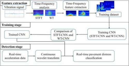
Figure 1 shows the framework of a novel pavement transverse cracks detection model for the classification of deep learning process including three phases: the feature extraction by STFT and WT; the training data by CNN, and the detection and classification of pavement conditions. In the feature extraction stage, the acceleration data expressed in the time–acceleration domain is transformed into an image with a time–frequency-energy domain by the WT based on the morce mother wavelet STFT with a window of 0.5 s, respectively. All data obtained from the driving test are stored as images converted to STFT and WT and used as a training dataset for CNN. When the CNN is trained by the STFT and WT training data sets in the training stage, the trained STFT-CNN and WT-CNN are created. Finally, in the pavement transverse cracks detection stage, the data collected from the site are converted by STFT and WT, and then detected and classified by trained STFT-CNN and WT-CNN. The effectiveness of different time–frequency analysis methods combined with CNN is compared with the detection accuracy of different networks for the same signal data. The time–frequency analysis for signal extraction and identification has been applied to EGG signal identification and mechanical vibration signals (Duan et al. 2019). The proposed WT-CNN and STFT-CNN for pavement feedback signals are pre-processed with a layer of signal to convert vibration signals into time–frequency images. And based on the transfer learning approach (Manikonda and Gaonkar 2019), the network structure is fine-tuned based on the VGG16 pre-training model to achieve the detection of transverse cracks in pavements.

Figure 1. Framework of a novel pavement transverse cracks detection model.

2.1. Methodology: time–frequency domain analysis

The amplitude of the acceleration is peaking up when the vehicle passes on the transverse cracks of pavement, but the amplitude of the signal is not able to be a criterion classifying the transverse cracks types. It depends on the various collision conditions between the wheels and the transverse cracks of the pavement. Therefore, the time–amplitude domain was converted to time–frequency domain in this paper to find a specific signal for each transverse cracks of pavement. Short-time fast Fourier transform and wavelet transform were used for time–frequency domain analysis in this paper.

2.1.1. Short-time fast Fourier transform (STFT)

Gabor (1946) improved the Fourier transform by introducing the ‘window’ concept (Cohn 1995). The short-time Fourier transform (STFT) is one of the most commonly used methods that the signal to be transformed is multiplied by a non-zero window function and the window function shifts along the axis of time (Chen et al. 2019a, 2019b, 2021). The Fourier Transform is implemented in every window and the obtained spectrum can be expanded into a two-dimensional image which can reflect the frequency change over time. The transferred frequency–time domain can be defined as Equation (1), where, $w[n-T]$ is the window function and $x[n]$ is the signal to be transformed (Han et al. 2015). (1) $STFT(\omega ,T)=\sum _{n=0}^{N-1}x[n].\omega [n-T]e^{-j\omega n}$(1)

The window size has to be wide enough to ensure that the input signal’s target portion is contained in the window, but a wide window size can provide low frequency resolution, and a narrow window size cannot provide sufficient time separation. In this paper, the window size was set to 0.5 s to satisfy the two conditions of including the specific frequency of the response between the wheel and the road surface in the window and maintaining an interpretable resolution.

2.1.2. Wavelet transform (WT)

Since the result of the transformed signal in SFTF analysis is always influenced by the window size, in order to minimise this effect, wavelet transform (WT) analysis, which can perform automatic adjustment of the window size, was used in this paper as well. After the signal is evaluated by a wavelet function, the signal is transformed separately for different segments of the time-domain signal. The wavelet is defined by Equation (2) (Zheng et al. 2002): (2) $WT(s,u)={\displaystyle \frac{1}{\sqrt{S}}{\int }^x[t]\psi \left({\displaystyle \frac{t-u}{s}}\right)dt}$(2) where, u and s are the shift and scale parameters, respectively. u is the wavelet’s position along with the signal so that WT(s, u) can get the similarity between the signals at time t, and the change of u will affect the position of the timeline in the centre of the corresponding time–frequency window. If s increases, the centre frequency of the time–frequency window decreases and the central time increases (Yoo and Baek 2018). The wavelet base function ${\psi }_{su}$ is defined by Equation (3): (3) ${\psi }_{su}(t)={\displaystyle \frac{1}{\sqrt{S}}\psi \left({\displaystyle \frac{t-u}{s}}\right)}$(3)

The morce wavelet was used as the generating function,$\psi (t)$, for time–frequency analysis. For a given signal, the wavelet coefficient can be expressed as a complex conjugate. The WT can be used to obtain frequency and spatial information to better visualise the frequency components of various scales and resolutions. (4) $\psi (t)=e^{-{\displaystyle \frac{t^2}{2}}}{e}^{-i{\omega }_{0}t}$(4) (5) $\psi (t)=\sqrt{2\pi }{e}^{{\displaystyle \frac{{(s-u)}^2}{2}}}$(5)

2.2. Overview for convolutional neural network

As a typical end-to-end deep learning model, CNN can take the original vibration signal as input and adaptively train the convolution kernel as a filter to extract transverse cracks features(Pang et al. 2017). However, CNN can only distinguish transverse cracks-related feature components by training different convolution kernels when classifying aliasing signals, which makes it difficult to distinguish transverse cracks-related features from other features in the hidden layer. Because time–frequency analysis can effectively extract the required feature components from the signal, and CNN is susceptible to interference from other vibration components when training the convolution kernel, a detection system combining time–frequency analysis and CNN is proposed.

Deep convolutional neural network(DCNN) usually needs a large number of annotation of image data sets to achieve higher prediction precision, but it is difficult to access a large amount of data for various reasons (Gopalakrishnan et al. 2017). Therefore, using a DCNN network that has been pre-trained on an annotated image dataset can avoid parameter adjustment and other processes. Transfer learning was proved very useful for solving cross-domain image classification problems (Shin et al. 2016). It is effective to use pre-trained deep learning and transfer their learning capabilities to new classification schemes instead of training new DCNN classifiers from scratch (Bar et al. 2015). Pre-trained DCNNs with proper fine-tuning are more applicable than DCNNs trained by scratch for some imaging applications (Tajbakhsh et al. 2016).

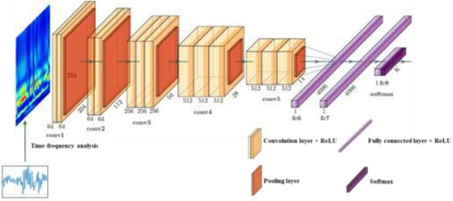
The model’s parameter scale is greatly reduced by the structure of the convolutional neural network local connection and weight sharing. A trainable and adjustable bias can be added by each channel on the output feature graph filtered by the convolution layer. The results obtained by the operation of the convolution layer have to be entered as a nonlinear activation function in order to ensure that the convolutional neural network has nonlinear fitting capabilities. Each type of CNN architecture includes nearly the same core artefacts: convolution layer, pooling layer, full connection layer and softmax layer as shown in Figure 2 (Ibragimov et al. 2020).

Figure 2. The architecture of the proposed CNN model.

Convolutional layer: The convolutional layer, a key component of a CNN, has two features: weight sharing and local connection. These two functions reduce the scale of the network structure parameters, thus reducing machine overfitting due to many parameters. A convolution kernel is used in the convolutional layer to perform convolution operations on the input signal to produce corresponding features.

Activation function: The activation function is an important part of the convolutional neural network. The activation function was introduced to increase the neural network model’s nonlinearity and is recommended to be applied to complex projects. The selection of an appropriate activation function has a positive influence on the improving the training speed of the convolutional neural network. The main purpose of the activation function is to enhance the linear divisibility of the originally linearly indivisible multi-dimensional features in another space of the map. The ReLU (Rectified Linear Unit) activation function used in this study is generally used in convolutional neural networks and can overcome the gradient dispersion phenomenon well.

Pooling layer: The feature map of the input image generated by convolution is used as input data for classification. The dimension of the feature vector of the convolution is large; hence, the classifier not only computes too much, but also overfitting. A nonlinear down-sampling method for the extraction of signals is adopted in the pooling layer (Liu et al. 2018). In this paper, a pooling process is performed to reduce the dimensions of the features at different positions aggregated for statistics in the image. There are usually two pooling methods: maximum pooling and mean pooling. The filter size was set to 2 × 2 in sampling because a large filter causes a large loss of information. Max pooling generally can retain more detailed features, while mean pooling can retain more global features. The sampled information after the mean pooling sampling is multiplied with a trainable training parameter and then it is added as a trainable bias. The resulting value can be calculated by the activation function to obtain the output of the current neuron. One of the most popular is maximum pooling. The main function of the pooling layer is to reduce the number of parameters and computation in the network. In addition, the layer can control that the over-fitting pooling layer always runs after each convolution layer.

Fully-connected layer: The main function of the fully-connected output layer is to classify the features extracted from the front-end network. Each neuron in the full connectivity layer is fully connected to all neurons in the previous layer. Dropout can be introduced at the full connection layer to prevent over-fitting during training (Wu and Gu 2015). Some neurons can be discarded with a certain probability during each iteration of training the neural network, and the output of discarded neurons is set to zero and the update is stopped. Based on this process, the generalisation ability of the network is improved and overfitting can be prevented.

Softmax layer: The main role of the Softmax layer is to predict classes based on features extracted from the full connection layer. This layer evaluates all the characteristics of the full connection layer and calculates the probability of each individual class. Then, the highest probability of a class is printed as the classification result.

3. Data acquisition and raw signal labelling and segmentation

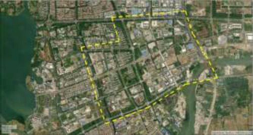
In order to identify a novel pavement crack detection model proposed in this paper, the signals regarding road surface condition were collected during the driving test on the selected route. The test route is located in Suzhou Industrial Park, China as shown in Figure 3. In the designated test route, there were structures inevitably installed on the road as well as transverse cracks of pavement, and the reaction of sensors by these road conditions was collected during the driving test.

Figure 3. Experimental area.

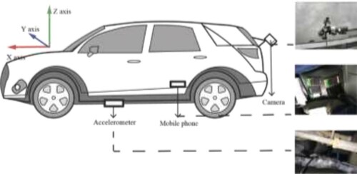
In order to better distinguish road conditions in the selected route, a camera was mounted on the rear of the vehicle to record road images. At the same time, it is possible to collect vibration information from the pavement during a driving test by three smartphones each equipped with an accelerometer and an accurate accelerometer installed next to the vehicle wheel. As shown in Figure 4, the phone is secured to the second row of seats in the vehicle, positioned close to the vehicle chassis. Before the data collection, the position of the device is adjusted to ensure that the mobile phone is placed horizontally so as to fully collect the change of Z-axis acceleration. In order to record the actual vibration of the vehicle body more accurately and verify the accuracy of the vibration signal collected by the phone, an accelerometer is installed on the chassis of the vehicle to ensure that the vibration signal from the chassis is fully captured. The sampling rate of accelerometers in smartphones and an accurate acceleration are 100 Hz. The installation of the equipment is shown in Figure 4. The amplitude and frequency of the signal can be affected by the vehicle speed (Sun 2003), the test vehicle was driven at a speed of about 30 km/h to acquire uniform data.

Figure 4. Layout of equipment.

Figure 5 shows the segmentation procedure of acceleration data to label the ground truth of the crack data. After collecting the acceleration signal from each type of road surface, the time through which the transverse cracks to the pavement and manhole has passed can be displayed by manually checking the image frame by frame. This time can be compared with the time of acceleration data to segment transverse cracks or acceleration signals of road structures. Then, each acceleration signal has been labelled with corresponding road condition. After collection and segmentation of data, around 2700 acceleration signals including transverse cracks and pavement structures were stored as a data set.

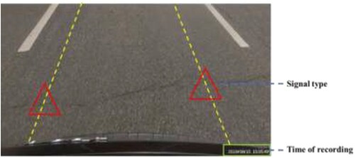
Figure 5. Schematic diagram of the signal labelling method.

3.1. Performance comparison between smartphone sensor and professional sensors

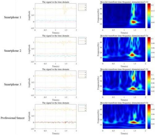
There are differences in their measurement sensitivity and acquisition stability as well as sampling frequency depending on the type of accelerometer. Figure 6 shows samples data from three smartphone sensors and a professional sensor, which is to verify that the same feature spectrum can be obtained after the Time–frequency analysis even though there are differences in acquisition accuracy and range between different sensors. The placement of three mobile phones are approximately the same location on the seats during the experiment, but the sensitivity of the sampling is not same due to different data collection frequency. The amplitude of the different sensors is not the same as shown in Figure 6 when the vehicle passed on the same crack, and hence the vibration signal is not able to distinguish simply different types of signals. In contrast, the signal coherence and the sensitivity of the professional sensor is better. However, after time–frequency analysis, these different vibration signals can be extracted and the characteristic frequency with the maximum energy is around 10 Hz. Yang and Zhou (2020) also verified that the appearance of transverse cracks leads to a sharp increase in energy in the sensitive frequency band of 10 ∼ 20 Hz. The results of this paper also proved that the sensors of the mobile phone are also sufficient for the detection and identification of cracks in the road surface after the data transformation into the time–frequency domain.

Figure 6. Performance comparison between smartphone sensor and professional sensors.

3.2. Time–frequency analysis results comparing STFT and WT

The acceleration is not only affected by the field conditions and vehicle type, but also the amplitude of the acceleration is changed depending on the collision conditions between the wheels and cracks of the pavement. Therefore, vibration data expressed in the time–amplitude domain is not able to provide appropriate for each type of crack in CNN analysis. However, when the vibration data expressed in the time–amplitude domain is transformed in the time–frequency domain, the features of the data can be derived with a specific frequency generated by the collision between the wheel and each crack. Therefore, in this paper, data transform was attempted by the STFT and WT methods, and the transformed data was used as an input for CNN analysis.

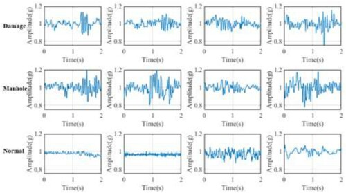
A fixed window function is used in STFT analysis, but once the window function is selected, its size is not able to be changed, which means that the resolution of the STFT is determined. STFT is mainly used to analyse segmented stationary signals or approximate stationary signals, which are mainly a waveform. However, for non-stationary signals such as road transverse cracks signals, when the signal changes drastically, the window function with a smaller window size of the STFT is required to have a higher time resolution. Window function with a larger window size is required to have a higher frequency resolution when the low frequency signal is changed relatively gently. Therefore, the STFT is not able to take into account both the frequency and the time resolution requirements during the computation. However, wavelet transform is possible to use a cluster of wavelet functions to represent or approximate the signal and hence it can take into account both frequency and time resolution in signal analysis. In order to compare the performance of different time–frequency analysis methods in this paper, STFT and WT were used to extract the time–frequency spectrum matrix of road signals. WT has high resolution characteristics and it is able to characterise the local characteristics of signals in both the time and frequency domains. The fundamental wave of the Fourier transform is a sine wave, and the transformed signal is regular and predictable without selected a window. The wavelet base of the wavelet transform is different from the Fourier transform, so that it is necessary to select a suitable wavelet base when using the wavelet transform. Wavelet bases have irregularities, and the shape and regularity of different wavelet bases vary widely. The results are different because the same signal is processed with different wavelet bases. Therefore, the selection of wavelet basis is an important factor in obtaining the appropriate result in signal processing using wavelet analysis. The linear transform has an appropriate result when analysing a signal that frequency changes gradually. In practical applications, since the wavelet basis and decomposition scale of the wavelet transform need to be based on different characteristics of the signal to be processed, it can be finally selected by many experiments. The classification basis examples of vibration signal is shown in Figure 7 and the segmented original vibration signal is shown in Figure 8. In a time-domain vibration signal, the horizontal and vertical axes represent time and amplitude, respectively. The unit is gravity (g), which represents the acceleration of gravity, and is commonly used to define the amplitude. The vibration signal caused by vehicles passing on pavement damage contains information that can be used to predict road transverse cracks. However, since the amplitude can be changed according to the collision pattern between the transverse cracks of the road surface and the vehicle wheel, it is not able to be a standard for transverse cracks detection.

Figure 7. Classification basis examples of vibration signal.

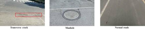
Figure 8. Raw acceleration data.

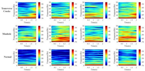
The original vibration signal is transferred by STFT to extract the feature of the signal. In this paper, in order to determine the optimal STFT window size to include a signal that reflects transverse cracks without the resolution reduction, segmented signals were analysed by STFT, and the window size that best reflects the two conditions was 0.5 s. Figure 9 shows the result of STFT transform of the original data with a window size of 0.5 s, and examples of the results for the pavement transverse cracks, the manhole, and the normal road. In order to show more distribution characteristics of the low-energy spectrum, the power spectral density (PSD) obtained after the Fourier transform is transformed to 20*log10(PSD), which is presented as the signal energy value in Figure 9. In normal roads, the increase in energy for each frequency is not noticeable. However, in the case of the manhole, the energy change occurs between the frequency of 10–15 Hz, and the energy increases over the entire region of 1 s. In the case of transverse cracks, a change in energy occurs for 0.5 s at a frequency of about 12 Hz. When vehicle passed on the damaged road, the amplitude of the signal is increased up to 1.2 G, but it can be variable due to the damaged types and conditions. Therefore, transverse cracks types are not able to be distinguished by the amplitude of signal. But in the time–frequency domain, a unique frequency range can be found according to the condition of the road surface.

Figure 9. Spectrum of STFT time–frequency analysis.

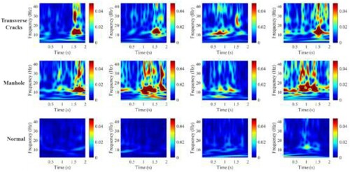
The wavelet power spectrum generated by morce-based WT is applied this this paper as well. Figure 10 shows the transferred signal for three cases: transverse crack surface; the manhole; and the normal road surface, in time–frequency domain, which can show the energy distribution of vibration signals based on image features as well. Figure 10 shows that the amplitude of collected signal is relatively low when passing on a normal road, and there is no apparent periodicity of the energy distribution. However, when passing on a damaged pavement, it will have a visible characteristic frequency of the spectrum, which is mainly distributed between 10 and 20 Hz and also there are some high-frequency scattered characteristic signals in the spectrum. When passing through the manhole, the characteristic frequency of the vibration is relatively scattered and has a longer duration. Comparing the ability of STFT and WT to extract time–frequency signals as shown in Figures 9 and 10, it can be clearly found that the frequency of WT extraction clearly distinguishes the transverse cracks types. Because the spectrum of the STFT is limited by the window size, the information of frequency and energy are dispersed on the time axis, which makes the spectrum loss the ability to distinguish the changes with the time. It is also difficult to distinguish the signal from the damaged road. However, it is still difficult to distinguish manually by the characteristic distribution of the signals in both methods.

Figure 10. Spectrum of WT time–frequency analysis.

4. Results and discussion

In the raw data processing phase, data cutting by recorded time and establishing dataset was done. Then, when constructing the time–frequency model, the original signal set needs to be extracted the time–frequency matrix features of the samples by time–frequency transformation methods such as STFT and WT. MATLAB 2019b is used for the data analysis.

During each round of training, 70% of the total 7680 samples are randomly selected as the training set, and the remaining samples constitute the test set. The details of the dataset are shown in Table 1. These samples will not be used for model training, but only used to evaluate model performance. The proposed deep learning network used Matlab 2019b to build the model with Intel Core i5 9400 f (6 cores) microprocessor, 32 GB of RAM and NVIDIA GeForce GTX1070 graphics processing unit (GPU) to carry out the training of the classification model. Two-dimensional data based on the time–frequency domain characteristic matrix of samples are trained and classified by the proposed CNN model. Image batch size is set to 16, and for all the training of the model for a period of up to 100 epochs using the early stop standard, the final model is the validation of low loss model using pre-trained VGG16 DCNN with Adam optimiser. The curve of training and validation accuracy and loss of STFT-CNN and WT-CNN are shown in Figures 11 and 12. The mean accuracy of the WT-CNN model is 97.2%, and with the loss value 0.22. The mean accuracy of STFT-CNN is 91.4%, which is slightly lower than that of WT-CNN, and the loss is 0.25. If the loss is smaller, the network optimisation is generally higher. At the same time, it is sufficient to enable real-time analysis in terms of the detection efficiency in the network. It takes 160 min and 28 s to train the WT-CNN detection network and 157 min and 57 s to train the STFT-CNN detection network on a single Nvidia GTX1070 GPU card. However, in the inference stage, the calculation is almost real-time. WT-CNN and STFT-CNN are used to infer two thousand sets of data. It takes 20.26 and 20.17 s, respectively and hence the average inference time is about 0.01 s. This results show that the WT-CNN has higher accuracy for detecting transverse cracks of the pavement, that also proves the validity of the combination of the time–frequency domain feature matrix and CNN proposed in this paper.

Figure 11. Training and validation accuracy and loss with ImageNet pre-trained VGG-16 DCNN deep image extractors with STFT feature for transverse cracks detection.

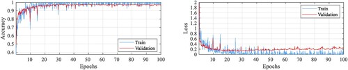
Figure 12. Training and validation accuracy and loss with ImageNet pre-trained VGG-16 DCNN deep image extractors with WT feature for transverse cracks detection.

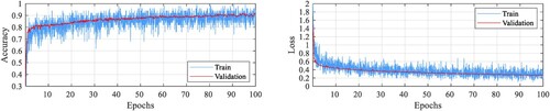
Table 1. Samples of each dataset.

Method	STFT-CNN			WT-CNN
Categories	Transverse cracks	Manhole	Normal	Transverse cracks	Manhole	Normal
Number of training samples	1792	1792	1792	1792	1792	1792
Number of validation samples	768	768	768	768	768	768
Total	2560	2560	2560	2560	2560	2560

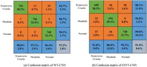
Figure 13 shows the confusion matrix for WT-CNN and STFT-CNN. Figure 13(a) shows that the WT-CNN can accurately determine the signal type and achieved an accuracy of 97.2%. Since features of the spectrum between the transverse cracks signal and the signal of the normal road are clearly distinguished, it is possible for the transverse cracks signal to be accurately classified from the signal of the normal road. However, the signal of manhole tends to be classified as the transverse cracks, and the normal road as well. The accuracy of STFT-CNN is 91.4%, which is more misclassified than WT-CNN (see Figure 13(b)). The tendency to misclassify signal types in STFT-CNN is similar to that of WT-CNN, but with a higher probability of misclassification. The manhole and the normal road are incorrectly classified as transverse cracks, resulting in lower classification accuracy for each category. It means that the information of signals in the STFT-CNN is lost more than that of WT-CNN. It is also verified that the WT method has a better effect of signal feature extraction compared with the STFT method.

1. Confusion matrix of WT-CNN

2. Confusion matrix of STFT-CNN

Figure 13. Confusion matrix.

In order to evaluate the classification effectiveness of the model, the Recall, Precision, Accuracy and F1-score are used as the evaluation indicators in this paper. The accuracy shows the ability to accurately distinguish road transverse cracks signals and non-transverse cracks signals. The Precision reflects that detection ability of the system, and also means whether it effectively identify the transverse cracks signal. The recall is the standard of ability to find out of whole transverse cracks signal. F1-score is a composite indicator of the detection system, and the high value of F1-score means the detection ability is high. The indicators are calculated by the confusion matrix of these Variables calculated by the Equations (6)–(9), respectively, the real positive (TP) classifier said the number of correctly predicted pavement signal types, false positives (FP) corresponding to the vibration signal was mistakenly classified the number of false negatives (FN) instructions to predict several other categories. (6) $\mathrm{Recall}={\displaystyle \frac{TP}{TP+FN}}$(6) (7) $\mathrm{Precision}={\displaystyle \frac{TP}{TP+FP}}$(7) (8) $\mathrm{Accuracy}={\displaystyle \frac{TP+TN}{TP+FP+TN+FN}}$(8) (9) $F1-score=2\times {\displaystyle \frac{Precision\times Recall}{Precision+Recall}}$(9)

Table 2 shows the performance evaluation of the two methods in detail and all the indicator of WT-CNN is higher than STFT-CNN for the transverse cracks detection task. The WT-CNN has a 97.53% of accuracy in distinguishing the transverse cracks signals, which performs better than the STFT-CNN with 91.02% of accuracy. It means that the WT-CNN has the ability to accurately classify the signal. The precision of the WT-CNN is 94.72% higher than 88.15% of the STFT-CNN, which means the WT-CNN can detect the transverse cracks better than the STFT-CNN. The recall to show the ability to find out all the transverse cracks of WT-CNN is 98.05% also higher than 92.93% of STFT-CNN. The F1-score of WT-CNN is 96.35% higher than 89.56% of STFT-CNN, which means that the WT-CNN has a better balance between the Precision and the Recall. Therefore, the performance of the WT-CNN is higher than that of STFT-CNN which can accurately and thoroughly find out transverse cracks.

Table 2. Comparison of pavement transverse cracks detection results using WT-CNN and STFT-CNN.

Standard for evaluation	WT-CNN	STFT-CNN
Accuracy	97.53%	91.02%
Precision	94.72%	88.15%
Recall	98.05%	92.93%
F1-sore	96.35%	89.56%

Table 3 shows the comparison with other detection method in detection accuracy and cost. The laser sensor with its high data precision can better obtain the detailed size and depth characteristics of the cracks. Stereo vision can also obtain its depth information. Zhang et al. (2018a) used Kinect to capture its 3D information and obtained 89.09% segmentation accuracy. Its cost was well controlled with the $199 equipment cost. Zhou and Song (2020) used deep learning to detect cracks using laser-scanned range images and obtained an average accuracy of 99.6%. Zhang et al. (2018b) used laser sensors to capture 3D data of pavement and achieved an average detection accuracy of 98%. However, the detailed equipment prices. In proposed method, as it does not require new equipment to be purchased. The detect task can be done entirely using a smart phone and achieved 97.2% recognition rate. The STFT as well as the WT can extract the time–frequency features well, allowing to distinguish the vibration signals for recognition. It is possible to use low-cost equipment to detect pavements within an effective range of detection accuracy under the driving of big data.

Table 3. Comparison with pavement crack method.

Methods	Data type	Accurancy (%)	Equipment cost (estimate)
Zhang et al. (2018a)	RGB image (Kinect-Based)	89.09	$199
Zhou and Song (2020)	laser-scanned range images	99.6 (average)	none
Zhang et al. (2018b)	3D laser scaning	Over 98	none
Ours method	vibration signal	97.20	none

5. Conclusion and future work

In this paper, a novel pavement crack detection model is proposed to detect cracks based on acceleration data collected by smartphones. Since the features of cracks is not able to be accurately expressed by acceleration data, the acceleration-time domain data is transformed to the frequency–time-energy domain using the STFT and WT methods in this paper. The transformed data was used as input data to distinguish cracks, manholes, and normal roads, and the STFT-CNN and WT-CNN models were compared with each other. The detailed conclusions of this paper are as follows:

1. 7680 data sets obtained from smartphones were collected for transverse cracks, manholes, and normal roads during the driving test. The gravitational acceleration, which represents the amplitude of the acquired raw data, was not used as a criterion for detecting cracks because it changes according to the collision conditions between the vehicle’s wheels and transverse cracks. In the result transformed by STFT, the energy change of the manhole continued for about 1 s at a frequency between 10 and 15 Hz, and in the case of transverse cracks, the energy changed at about 12 Hz for about 0.5 s. In the result of the WT method, the energy change between the manhole and the transverse cracks occurred between 10 and 20 Hz, but it was maintained for a longer time in the manhole. The data transformed by STFT and WT were used as input data of STFT-CNN and WT-CNN, which classifies transverse cracks, manholes, and general roads.

2. The mean accuracy of the WT-CNN model is 97.2%, and with the loss value 0.22. The accuracy of the STFT-CNN is 91.4%, which is slightly lower than that of WT-CNN, and the loss is 0.25. This results show that the WT-CNN has higher accuracy for detecting transverse cracks of the pavement, that also proves the validity of the combination of the time–frequency domain feature matrix and CNN proposed in this paper.

3. Since features of the spectrum between the transverse cracks signal and the signal of the normal road are clearly distinguished, it is possible for the transverse cracks signal to be accurately classified from the signal of the normal road. However, the signal of manhole tends to be classified as the transverse cracks, and the normal road as well. This tendency to misclassify signal types is similar for both the STFT-CNN and the WT-CNN, but STFT-CNN is lower accuracy to classify each type. It is verified that the WT method has a better effect of signal feature extraction compared with the STFT method.

4. The F1-score of WT-CNN is 96.35% higher than 89.56% of STFT-CNN, which means that the WT-CNN has a better balance between the Precision and the Recall. This result is reflected that the WT-CNN has a better performance of pavement transverse cracks detection than STFT-CNN.

This paper has conducted numerous experiments with a single vehicle. However, there are still various factors that affect acceleration, such as the type and condition of the vehicle and the driving condition of the driver. Therefore, the analysis method of this paper needs to be used under a wider range of vehicle, pavement and driving conditions.

Disclosure statement

No potential conflict of interest was reported by the author(s).

References

- Bar, Y., et al., 2015. Chest pathology detection using deep learning with non-medical training. In: 2015, IEEE 12th international symposium on biomedical imaging (ISBI). IEEE.Brooklyn, NY, USA, 16-19 April 2015
- Chen, C., et al., 2019a. Pavement damage detection system using big data analysis of multiple sensor. In: International conference on smart infrastructure and construction 2019 (ICSIC) driving data-informed decision-making. ICE Publishing.Cambridge, UK, July 05, 2019
- Chen, C., et al., 2019b. Automatic pavement crack detection based on image recognition. In: International conference on smart infrastructure and construction 2019 (ICSIC) driving data-informed decision-making. ICE Publishing.Cambridge, UK, July 05, 2019
- Chen, C., et al., 2021. Pavement crack detection and classification based on fusion feature of LBP and PCA with SVM. International Journal of Pavement Engineering, https://doi.org/10.1080/10298436.2021.1888092.
- Cohn, L., 1995. Time-Frequency analysis: theory and applications. Englewood Cliffs: Prentice Hall.
- Duan, S., Zheng, H., and Liu, J., 2019. A novel classification method for flutter signals based on the CNN and STFT. International Journal of Aerospace Engineering, 2019, 1–8.
- Fan, Z., et al., 2020a. Ensemble of deep convolutional neural networks for automatic pavement crack detection and measurement. Coatings, 10, 152. https://doi.org/10.3390/coatings10020152.
- Fan, Z., et al., 2020b. Automatic crack detection on road pavements using encoder-decoder architecture. Materials, 13, 2960. https://doi.org/10.3390/ma13132960.
- Fan, W. and Qiao, P., 2011. Vibration-based damage identification methods: a review and comparative study. Structural Health Monitoring, 10 (1), 83–111.
- Frank, P.M. and Ding, X., 1994. Frequency domain approach to optimally robust residual generation and evaluation for model-based fault diagnosis. Automatica, 30 (5), 789–804.
- Gabor, D., 1946. Theory of communication. Journal of the Institution of Electrical Engineers – Part III: Radio and Communication Engineering, 93, 429–441.
- González, A., et al., 2008. The use of vehicle acceleration measurements to estimate road roughness. Vehicle System Dynamics, 46 (6), 483–499.
- Gopalakrishnan, K., et al., 2017. Deep Convolutional Neural Networks with transfer learning for computer vision-based data-driven pavement distress detection. Construction and Building Materials, 157, 322–330.
- Gupta, M., et al., 2015. A comparison between smartphone sensors and bespoke sensor devices for wheelchair accessibility studies. In: 2015 IEEE tenth international conference on intelligent sensors, sensor networks and information processing (ISSNIP). IEEE.Singapore, 22-24, April, 2015
- Han, D., Renaudin, V., and Ortiz, M., 2015. Smartphone based gait analysis using STFT and wavelet for indoor navigation. In: International conference on indoor positioning & indoor navigation.Busan, South Korea , 27-30 Oct. 2014
- Ibragimov, E, et al., 2020. Automated pavement distress detection using region based convolutional neural networks. International Journal of Pavement Engineering, 1–12. https://doi.org/10.1080/10298436.2020.1833204.
- Islam, S, et al., 2014. Measurement of pavement roughness using android-based smartphone application. Transportation Research Record, 2457 (1), 30–38.
- Kumar, A., et al., 2017. An ensemble of fine-tuned convolutional neural networks for medical image classification. IEEE Journal of Biomedical and Health Informatics, 21, 31–40.
- Kumaran, S.T., et al., 2017. Prediction of surface roughness in abrasive water jet machining of CFRP composites using regression analysis. Journal of Alloys and Compounds, 724, 1037–1045.
- Li, G., et al., 2019. Sensor data-driven bearing fault diagnosis based on Deep Convolutional Neural Networks and S-transform. Sensors, 19 (12), 2750. https://doi.org/10.3390/s19122750.
- Liu, Z., et al., 2018. GMM and CNN hybrid method for short utterance speaker recognition. IEEE Transactions on Industrial Informatics, 14 (7), 3244–3252.
- Manikonda, S.K. and Gaonkar, D.N., 2019. A novel islanding detection method based on transfer learning technique using VGG16 network. In: 2019 IEEE international conference on sustainable energy technologies and systems (ICSETS). IEEE, 109–114.Bhubaneswar, Odisha, 26 February 2019 – 01 March 2019
- Mohan, P., Padmanabhan, V.N., and Ramjee, R., 2008. Nericell: rich monitoring of road and traffic conditions using mobile smartphones. In: Proceedings of the 6th ACM conference on Embedded network sensor systems. ACM.Raleigh, NC, USA, 5-7, November, 2008
- Ozaktas, H.M., et al., 1996. Digital computation of the fractional Fourier transform. IEEE Transactions on Signal Processing, 44 (9), 2141–2150.
- Pang, S., Yu, Z., and Orgun, M.A., 2017. A novel end-to-end classifier using domain transferred deep convolutional neural networks for biomedical images. Computer Methods and Programs in Biomedicine, 140, 283–293.
- Pelecanos L., et al., 2018. Distributed fibre optic sensing of axially loaded bored piles. Journal of Geotechnical and Geoenvironmental Engineering, ASCE, 144 (3), 1–16.
- Ronneberger, O., Fischer, P., and Brox, T., 2015. U-net: convolutional networks for biomedical image segmentation. In: Proceedings of the 18th international conference on medical image computing and computer assisted intervention 2015, Munich, 5–9 October 2015. Berlin/Heidelberg: Springer, 9351, 234–241.
- Seo, H., et al., 2017. Crack detection in pillars using infrared thermographic imaging. Geotechnical Testing Journal, ASTM, 40 (3), 371–380.
- Seo, H., 2020. Monitoring of CFA pile test using three dimensional laser scanning and distributed fibre optic sensors. OpticS and Lasers in Engineering, 130, 106089. https://doi.org/10.1016/j.optlaseng.2020.106089.
- Seo, H., 2021a. Long-term monitoring of zigzag-shaped retaining structure using laser scanning and analysis of influencing factors. Optics and Lasers in Engineering, 139, 106498. https://doi.org/10.1016/j.optlaseng.2020.106498.
- Seo, H, 2021b. 3D roughness measurement of failure surface in CFA Pile samples using Three Dimensional laser scanning. Applied Sciences, 11 (6), 2713. https://doi.org/10.3390/app11062713.
- Seo, H., 2021c. Tilt mapping for zigzag-shaped concrete panel in retaining structure using terrestrial laser scanning. Journal of Civil Structural Health Monitoring, 150, 916. https://doi.org/10.1007/s13349-021-00484-x.
- Shin, H.-C., et al., 2016. Deep convolutional neural networks for computer-aided detection: CNN architectures, dataset characteristics and transfer learning. IEEE Transactions on Medical Imaging, 35 (5), 1285–1298.
- Simonyan, K. and Zisserman, A., 2015. Very deep convolutional networks for large-scale image recognition. arXiv preprint arXiv:1409.1556. 4 September 2014.ICLR 2015, 7 - 9, May, 2015
- Soga, K., et al., 2015. The role of distributed sensing in understanding the engineering performance of geotechnical structures. In: 2015, 15th European conference on soil mechanics and geotechnical engineering, Edinburgh, 13–17 September 2015.ICE Publishing.
- Sun, L, 2003. Simulation of pavement roughness and IRI based on power spectral density. Mathematics and Computers in Simulation, 61 (2), 77–88.
- Tajbakhsh, N., et al., 2016. Convolutional neural networks for medical image analysis: full training or fine tuning? IEEE Transactions on Medical Imaging, 35 (5), 1299–1312.
- Wang, Q. and Deng, X., 1999. Damage detection with spatial wavelets. International Journal of Solids and Structures, 36 (23), 3443–3468.
- Wang, W. and Guo, F., 2016. Roadlab: revamping road condition and road safety monitoring by crowdsourcing with smartphone app.Transportation Research Board 95th Annual Meeting, Washington DC, United States Date, 10-14 January, 2016.
- Wen, G., et al., 2017. Ensemble of Deep neural networks with probability-based fusion for facial expression recognition. Cognitive Computation, 9, 597–610.
- Wu, H. and Gu, X., 2015. Towards dropout training for convolutional neural networks. Neural Networks, 71, 1–10.
- Yagi, K., 2010. Extensional smartphone probe for road bump detection. In: 17th ITS World Congress ITS Japan ITS America ERTICO.17th ITS World Congress Location, Busan , South Korea, 25-29, October, 2010.
- Yang, Q. and Zhou, S., 2020. Identification of asphalt pavement transverse cracking based on vehicle vibration signal analysis. Road Materials and Pavement Design, 1–9.
- Yoo, Y. and Baek, J.-G, 2018. A novel image feature for the remaining useful lifetime prediction of bearings based on continuous wavelet transform and convolutional neural network. Applied Sciences, 8 (7), 1102. doi:10.3390/APP8071102.
- Zhang, Y., et al., 2018a. A kinect-based approach for 3D pavement surface reconstruction and cracking recognition. IEEE Transactions on Intelligent Transportation Systems, 19 (12), 3935–3946.
- Zhang, D., et al., 2018b. Automatic pavement defect detection using 3D laser profiling technology. Automation in Construction, 96, 350–365.
- Zheng, H., Li, Z., and Chen, X, 2002. Gear fault diagnosis based on continuous wavelet transform. Mechanical Systems and Signal Processing, 16 (2–3), 447–457.
- Zhou, S. and Song, W, 2020. Deep learning-based roadway crack classification using laser-scanned range images: A comparative study on hyperparameter selection. Automation in Construction, 114, 103171. https://doi.org/10.1016/j.autcon.2020.103171.