Resilient modulus estimation using in-situ modulus detector: performance and factors

ABSTRACT

The resilient modulus of subgrade should be estimated for pavement designs that undergo repetitive loading from vehicular movement. In this study, an in-situ modulus detector (IMD) with flat, wedge, and cone tips is employed to estimate the resilient modulus. The specimens with three different levels of water content are compacted, and the dynamic responses for two hammer drop heights are analysed. For all specimens, elastic waves are acquired to estimate the shear modulus and Poisson’s ratio using bender and piezo-disk elements. The resilient modulus estimated from the IMD is compared with the lightweight deflectometer (LWD) modulus. The experimental results show a stronger relationship between the flat and wedge tips than between the cone and wedge tips. Furthermore, higher drop heights result in strong relationships between the resilient, shear, and LWD moduli. This study proposes an intrinsic design and verification of an IMD for reliable resilient modulus estimation in pavement design.

KEYWORDS:

• Elastic wave
• in-situ test
• LWD
• resilient modulus
• subgrade

Introduction

The subgrade under the road serves as a foundation for the upper layers of road infrastructure. Subgrade strength, which can be expressed as load-carrying capacity, is an important parameter for pavement design (Peraka and Biligiri 2020). The California bearing ratio (CBR) test is a widely used laboratory test for assessing subgrade strength under pseudo-static loading. Previously, the CBR of a subgrade was estimated using a dynamic cone penetrometer (DCP) (Kleyn 1975, Webster et al. 1992, Gabr et al. 2000). However, when designing pavements, the resilient modulus of subgrade, which is measured under repetitive loading, should be considered to represent the stress state in pavements under wheel loads. To determine the resilient modulus of subgrade, repeated load triaxial tests are conducted as recommended by the American Association of State Highway and Transportation Officials (AASHTO). Nevertheless, high-quality core samples are required for repeated load triaxial tests. Moreover, field stress states that can influence the resilient modulus estimation are unknown.

Several field testing methods are used to evaluate the resilient modulus of subgrade. Non-destructive testing methods have been widely used in the field to evaluate the modulus of subgrade due to their fast and repeatable procedures. One of the most widely used testing methods for measuring pavement surface deflections is the falling-weight deflectometer (FWD). Back-calculation programmes can be used to determine the moduli of multiple layers in pavements after measuring a deflection basin (Li et al. 2018). However, such back-calculation programmes may not provide a unique set of elastic moduli for multi-layered pavements (AASHTO 2008). A lightweight deflectometer (LWD), which is a portable version of the FWD, can be used to control the subgrade compaction quality (Xu and Chang 2013, Schwartz et al. 2017, Duddu and Chennarapu 2022). Recently, Jibon and Mishra (2021) used LWD inside a Proctor mould to estimate the resilient modulus for different soil types and water contents. However, FWD and LWD can only be applied to ground surface, and their influence depth is limited to one to two times the diameter of the plate (Nazzal et al. 2004).

For deeper subgrade characterisation, intrusive testing methods have been employed. DCP is commonly used to investigate subgrade strength because DCP devices are portable and the test procedure to obtain a continuous subgrade profile is simple and quick. The dynamic cone penetration index (DCPI) measured along the depth can be used to generate subgrade strength profiles. DCPI can be correlated with the elastic modulus obtained from the LWD to estimate the stiffness profile of subgrade considering the strain influence factor along the depth (Schmertmann et al. 1978, Kim et al. 2021). An automated DCP was developed and compared with manual DCP devices to provide quick and reliable test results (Livneh et al. 1992). Several novel DCP devices have been proposed for reliable subgrade characterisation (Langton 1999, Byun and Lee 2013, Hong et al. 2017, Lee et al. 2019). Lightweight and instrumented DCP can provide dynamic resistance as a soil-resistance index by taking into account the transferred energies at the anvil and cone tip (Langton 1999, Lee et al. 2019). Crosshole-type DCP enables the estimation of shear moduli in subgrade, which are determined at low strain level (Hong et al. 2017). Recently, an in-situ modulus detector (IMD) was developed to provide resilient modulus profiles for subgrades (Byun and Kim 2022). However, various factors affecting the estimation of resilient moduli using the IMD have not been studied yet.

In this study, an IMD with different tip types was used to estimate the resilient modulus of subgrade with three different water contents for two different hammer drop heights. First, the IMD is introduced, followed by the test procedure and specimen preparation. Subsequently, the test results, including the dynamic response, modulus profiles, maximum shear modulus, and LWD modulus, are described. Finally, the effects of tip type and hammer drop height on the estimation of resilient modulus are discussed and compared to shear and LWD moduli.

Materials and methods

In-situ modulus detector

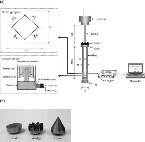
In this study, an IMD with various types of tip modules was developed to provide a resilient modulus profile of the subgrade. Figure 1 shows the shape of an IMD, which is composed of a tip module, hammer system, and driving rod. To investigate the effect of tip shape on resilient modulus estimation, three tip types were designed: flat, wedge, and cone, each with a diameter of 30 mm. To measure the dynamic force and displacement, four strain gauges and an accelerometer were installed at the tip module. The strain gauges were configured as a Wheatstone bridge circuit, which has been widely used for load cells owing to temperature compensation and bending effect minimisation (Byun and Lee 2013, Kim and Lee 2020). The load cell was calibrated to evaluate the force based on the output voltage measured at the tip module (Hong et al. 2022). To estimate the displacement, a piezoelectric accelerometer (PCB 350C03) with a maximum amplitude of 10,000 g was mounted on the tip module. The dynamic responses from the tip module were recorded and stored on a computer using a data logger at a sampling rate of 10 kHz. The hammer system comprised a hammer, guide, buffer, and anvil. The 43-N hammer and 685-mm-high guide were used to vary the potential energy of the hammer. The buffer and anvil were located between the guide and driving rod to transfer energy to the tip module, apply dynamic loads to subgrade, and minimise high-frequency noise in the force and acceleration signals. The length of the driving rod (1,000 mm) was the same as that of the DCP. The inner and outer diameters of the driving rod were 16 and 24 mm, respectively. Considering the difference in the diameters of the tip module and driving rod, side friction along the driving rod during penetration was negligible.

Figure 1. In situ modulus detector (IMD) (in mm): (a) schematic of the IMD and measurement system; and (b) picture of the three tip modules.

Specimens

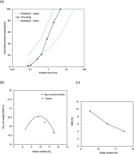
Weathered soil samples from Daegu, South Korea were used to prepare compacted specimens. Figure 2(a) depicts the particle size distribution curve of the weathered soil. A typical soil-aggregate material gradation specified by AASHTO M147-65 (2004) was added for comparison. The soil samples were compacted with three different water contents according to the ASTM D1557 (2012) specification. A Proctor mould with a height and diameter of 168 and 150 mm, respectively, was prepared; subsequently, each layer of soil was compacted with 56 blows for five layers using a 43-N hammer. After compaction with water contents of 9.5, 10.5, and 11.5%, the dry unit weights of the three specimens were 20.5, 20.2, and 19.6 kN/m³ respectively. The measured values were similar to the compaction curve provided by Byun and Kim (2022), as shown in Figure 2(b). Figure 2(c) shows that the CBR of the three specimens varies with water content, ranging from 9.5–4.0%.

Figure 2. Properties of sandy soil specimens: (a) particle-size distribution curve; (b) compaction curve; and (c) California bearing ratio (CBR).

Test procedure

The compacted specimens were subjected to dynamic penetration tests using an IMD. After compacting the specimens for each water content, a 53-N doughnut-type hammer was placed on the specimens to simulate a pavement above subgrade (Figure 3). Dynamic penetration tests were performed using an IMD by dropping the hammer and varying the drop height between 5 and 50 cm during penetration. These tests were performed up to a penetration depth of 9 cm, which allowed a 6-cm space from the bottom of the mould. After finishing the penetration, the remaining length of the specimen corresponded to the influence depth, which was twice the diameter of the plate. Regardless of the penetration depth, the dynamic penetration test was terminated when the blow count reached 50.

Figure 3. Experimental setup for (a) dynamic penetration test with elastic wave measurement and (b) lightweight deflectometer (LWD) test.

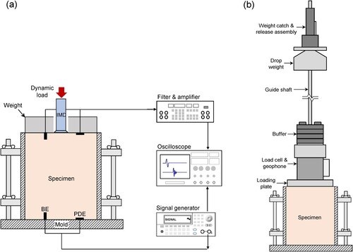
For all compacted specimens, elastic waves were measured to estimate the shear modulus and Poisson’s ratio. At the top and bottom of the mould, a pair of bender elements and piezo-disk elements were installed to generate and detect shear and compressional waves, respectively. The bender and piezo-disk elements at the bottom were connected to the signal generator to propagate the elastic waves, whereas the top ones were used to receive the wave signals. After filtration and amplification, the received wave signals were visualised using an oscilloscope, as shown in Figure 3(a). Another specimen compacted under the same conditions but without a doughnut-type weight was prepared for the LWD test, shown in Figure 3(b). The diameter of the loading plate of the LWD was slightly smaller than the inner diameter of the Proctor mould. Jibon and Mishra (2021) reported that the elastic moduli estimated using LWD on the Proctor mould are well correlated with the resilient moduli.

Results

Dynamic response

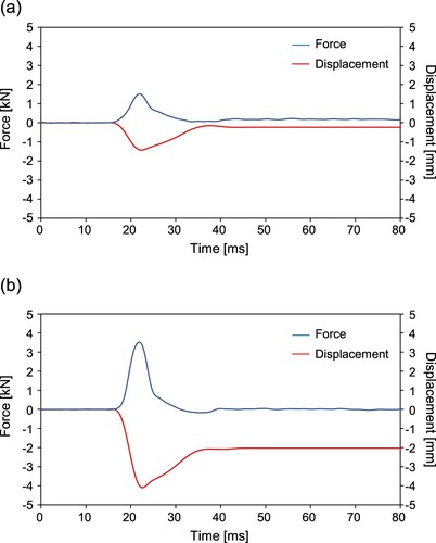
Dynamic responses were obtained from each blow in dynamic penetration tests with three tip shapes, three water contents, and two dropping heights. The dynamic force and displacement signals were measured using strain gauges and accelerometers installed at the tip module. Figure 4 shows the dynamic responses of a specimen with 10.5% water content when subjected to hammer drop heights of 5 and 50 cm. The dynamic responses of force and displacement were captured simultaneously (Figure 4). Because of the compressional force and downward movement, the force and displacement signals increased and decreased, respectively. Both signals exhibited peak amplitudes after dropping the hammer and converged when the compressional force dissipated and the displacement recovered. Because of the difference in transferred energy, the maximum amplitude of the force signal for the drop height of 5 cm was less than that for the drop height of 50 cm. Thus, the total and permanent displacements for a drop height of 5 cm were smaller than those for a drop height of 50 cm.

Figure 4. Force and displacement signals obtained using IMD at the specimens with 0.5% water content and hammer drop heights of (a) 5 cm and (b) 50 cm.

Based on the dynamic response measured using the IMD, the resilient modulus (M_r) of soil can be expressed as follows: (1) $M_r={\displaystyle \frac{{\sigma }_d}{{\epsilon }_r}}$(1) where σ_d and ϵ_r are the deviatoric stress and recoverable strain, respectively. The deviatoric stress was obtained from the maximum force measured by the load cell by assuming a parabolic distribution of the contact stress under the tip of the IMD. The recoverable strain is the recoverable displacement measured by the accelerometer divided by the influence depth of dynamic loading. Further details of M_r estimation, based on the dynamic response measured using IMD, can be found in Byun and Kim (2022).

Dynamic penetration profiles

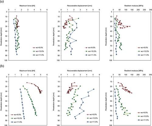
Typical profiles of the maximum force, recoverable displacement, and resilient modulus for the three specimens with different water contents are plotted in Figure 5. For a drop height of 5 cm, the maximum forces at lower water contents were slightly higher at the same penetration depths and the variation in maximum force with penetration depth was less significant. Regardless of the water content, the maximum forces for the drop height of 50 cm were greater than those for the drop height of 5 cm. For a drop height of 50 cm, the maximum force for the three water contents increased with penetration depth; this increase was greater at lower water contents. Overall, regardless of the drop height, a higher water content resulted in greater recoverable displacements at the same penetration depth. The recoverable displacement for a drop height of 5 cm was less than that for a drop height of 50 cm. The recoverable displacements for a drop height of 50 cm decreased with increasing penetration depth, showing some fluctuation. The variation in recoverable displacements with penetration depth was less significant for a drop height of 5 cm, especially at higher water contents. These findings are consistent with those reported by Byun and Kim (2022). The resilient modulus estimated from maximum forces and recoverable displacements increased with penetration depth, regardless of the drop height of hammer. The increase in the resilient modulus with penetration depth was greater at lower water contents than at higher water contents.

Figure 5. Dynamic penetration profiles for the wedge tip module for hammer drop heights of (a) 5 cm and (b) 50 cm.

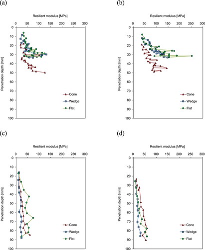
The resilient modulus profiles for hammer drop heights of 5 and 50 cm are plotted in Figure 6 to examine the effect of the tip type. Figures 6(a) and (b) show the resilient modulus profiles of the specimen with a water content of 9.5%. For dense specimens, the blow count reached 50 before the penetration depth of 9 cm. Among the tip types, the cone tip exhibited the deepest penetration depth owing to its sharp tip shape. For the water content of 9.5%, the resilient modulus obtained from the cone tip was lower than those obtained from the other tip types. The resilient modulus profiles for the specimen with a water content of 11.5% are shown in Figures 6(c) and (d). For the loose specimens, all tips reached the penetration depth of 9 cm before the blow count of 50. For the water content of 11.5%, the resilient modulus obtained from the wedge tip was lower than those obtained from the other tip types. Regardless of the water content, the flat tip exhibited a higher resilient modulus with greater fluctuations along the penetration depth for a drop height of 5 cm. Previous studies have shown that flat tips have a higher penetration resistance than cone tips (Kim et al. 2008, Tovar-Valencia et al. 2021).

Figure 6. Resilient modulus profiles with the penetration depth for water contents of 9.5%: (a) drop height of 5 cm and (b) drop height of 50 cm; and 11.5%: (c) drop height of 5 cm and (d) drop height of 50 cm.

Maximum shear modulus

After soil compaction, elastic waves were measured to estimate the shear modulus and Poisson’s ratio. For the three tip modules, specimens with water contents of 9.5, 10.5, and 11.5% were prepared; nine points of shear wave velocity and shear modulus are plotted in Figure 7. The shear wave velocity decreased linearly as the water content increased. The linear relationship between the shear wave velocity (V_s) and water content (wc) can be expressed as follows: (2) $V_s=-51.9\cdot wc+701(R^2=0.948)$(2) A decrease in the dry density of the compacted soil specimens reduced the shear wave velocity. The shear wave velocity can be used to estimate the maximum shear modulus (G_max) as follows: (3) $G_{max}=\rho \cdot V_s^2$(3) where ρ and V_s are the dry density of the soil specimen and the shear wave velocity, respectively. In addition, the shear modulus decreased linearly from 110 to 20 MPa as the water content increased. The relationship between shear modulus (G_max) and water content can be represented as follows: (4) $G_{max}=-36.6\cdot wc+444(R^2=0.894)$(4) The range of shear moduli in this study was similar to that reported in previous studies (Byun et al. 2018; Kim et al. 2021). It should be noted that the shear moduli in previous studies were also estimated at low confining pressures. Poisson’s ratio can be determined from the estimation of the compressional and shear wave velocities as follows: (5) $\upsilon ={\displaystyle \frac{1}{2}\cdot {\displaystyle \frac{V_p^2-2V_s^2}{V_p^2-V_s^2}}}$(5) where υ and V_p are Poisson’s ratio and compressional wave velocity, respectively. The compressional and shear wave velocities decreased with increasing water content (Table 1). The Poisson’s ratios of the specimens with water contents of 9.5, 10.5, and 11.5% were 0.29, 0.38, and 0.44, respectively.

Figure 7. Dynamic material properties of the compacted specimens at different water contents: (a) shear wave velocity; and (b) shear modulus.

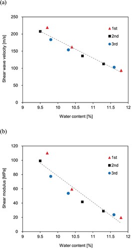
Table 1. Wave velocities and Poisson’s ratios estimated for specimens with different water content values.

Water content [%]	Compressional wave velocity [m/s]	Shear wave velocity [m/s]	Poisson’s ratio
9.5	377.1	203.4	0.29
10.5	337.5	150.6	0.38
11.5	314.0	103.2	0.44

LWD modulus

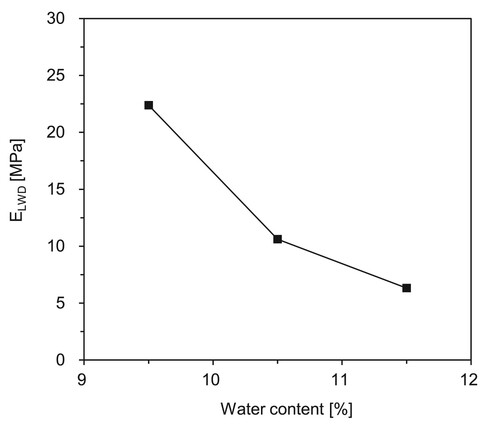
LWD testing was used inside the Proctor mould to measure the LWD modulus (E_LWD). The assumption of a semi-infinite half-space for estimating the modulus in standard LWD tests is not suitable for a confined state inside a mould (Schwartz et al. 2017). Considering the boundary limits of the mould, the LWD modulus can be estimated as follows: (6) $E_{LWD}=\left(1-{\displaystyle \frac{2\times {\upsilon }^2}{1-\upsilon }}\right)\times {\displaystyle \frac{4H}{\pi D^2}\times K}$(6) where H and D are the height and diameter of the mould, respectively, and K is the ratio of the peak force to the peak deflection. Eq. (6(6) $E_{LWD}=\left(1-{\displaystyle \frac{2\times {\upsilon }^2}{1-\upsilon }}\right)\times {\displaystyle \frac{4H}{\pi D^2}\times K}$(6) ) was derived from elasticity theory for cylindrical moulds with constrained lateral movement (Jibon and Mishra 2021). Herein, E_LWD decreased from 22.4–6.3 MPa as the water content increased (Figure 8), which is attributed to the decrease in the soil density with water content (Umashankar et al. 2016).

Figure 8. LWD results of the compacted specimens at different water contents.

Discussions

Repeatability

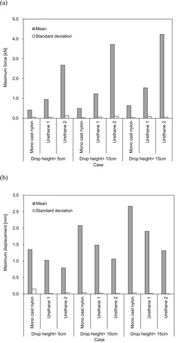
The dynamic responses obtained from three different materials reported by Kim and Byun (2019) were analysed to investigate the repeatability of dynamic response measurements in the IMD. In a previous study, the wedge tip of the IMD was placed on the surface of a sample and five different blows falling from drop heights of 5, 10, and 15 cm were applied to the buffer and anvil of the IMD. Figure 9 shows the mean and standard deviation of the maximum force and displacement measured by the load cell and accelerometer, respectively. Herein, the positive maximum displacement indicates that the tip is moving downward. Regardless of the type of material tested, the average values of both the maximum force and displacement increased with the drop height of hammer. For all cases, values of the standard deviation of maximum force and displacement were always equal to or smaller than 0.131 and 0.151, respectively. Except for the case of mono-cast nylon at a drop height of 5 cm, the coefficient of variation, defined as the ratio of standard deviation to mean, was less than 6% in the majority of cases.

Figure 9. Mean and standard deviation of dynamic response measured by using the IMD for three materials under three different drop heights: (a) maximum force; and (b) maximum displacement.

Effect of hammer drop height

The resilient moduli of specimens for different hammer drop heights and tip modules are shown in Figure 10. Regardless of tip shape, the resilient modulus of the specimens for the drop height of 50 cm was greater than that for the drop height of 5 cm. Linear functions can be used to represent the relationships between the resilient moduli for drop heights of 5 and 50 cm as follows: (7) $M_{r\mathrm{\_}50cm}=\alpha \cdot M_{r\mathrm{\_}5cm}$(7) where M_{r_5cm} and M_{r_50cm} denote the resilient moduli estimated at drop heights of 5 and 50 cm, respectively; and α is the slope of the linear relationship between the resilient moduli, which was determined using regression analysis. The values of the slope and coefficient of determination (R²) for the relationships of the resilient moduli for drop heights of 5 and 50 cm are summarised in Table 2. Figure 10(a) shows the linear relationship between the resilient moduli obtained for the cone tip. As the resilient modulus increased, the data points gradually scattered. For the wedge tip, the resilient moduli exhibited a linear relationship, as shown in Figure 10(b), with higher values of slope and R² than those of the other tip modules. For the flat tip, the linear relationship between the resilient modulus exhibited the lowest R² value, as shown in Figure 10(c). The data for the flat tip were dispersed at low resilient moduli. These results are consistent with high fluctuations in the resilient modulus profile for the flat tip, as shown in Figure 6. The resilient moduli averaged at depths of 25–35 cm for the three tip modules are shown in Figure 11. Without the effect of confining pressure, the resilient modulus of the specimens for a hammer drop height of 50 cm was greater than that for a hammer drop height of 5 cm for all tip modules. However, the hammer drop height had less of an effect on the estimated values at low resilient moduli than those at high resilient moduli.

Figure 10. Resilient moduli for different hammer drop heights and tip shapes: (a) cone; (b) wedge; and (c) flat. M_r denotes the resilient modulus estimated using IMD.

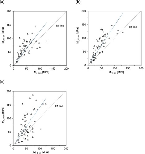
Figure 11. Resilient modulus averaged at depths of 25–35 mm for different hammer drop heights.

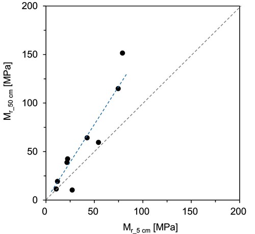
Table 2. Slope and coefficient of determination for three types of tip modules.

	Cone	Wedge	Flat	Average
Slope	1.26	1.48	1.41	1.56
Coefficient of determination	0.860	0.904	0.819	0.946

Effect of tip shape

Figure 12 compares the resilient moduli of the specimens subjected to the cone, wedge, and flat tip modules. Figure 12(a) shows the relationships between the resilient moduli estimated using the cone or flat tip and the wedge tip for a hammer drop height of 5 cm. Although the data were highly scattered, the linear relationship between the resilient moduli for the flat and wedge tip modules had a slope of 1, whereas the resilient modulus of the cone tip was lower than that of the wedge tip. These linear relationships can be represented as follows: (8) $M_{r\mathrm{\_}cone}=\beta \cdot M_{r\mathrm{\_}wedge}$(8) (9) $M_{r\mathrm{\_}flat}=\gamma \cdot M_{r\mathrm{\_}wedge}$(9) where M_{r_cone}, M_{r_wedge}, and M_{r_flat} denote the resilient moduli estimated from the cone, wedge, and flat tips, respectively. The values of the slopes of lines β and γ are summarised in Table 3. For a drop height of 50 cm, the relationship between the resilient modulus estimvnated using the cone or flat tips and the wedge tip is shown in Figure 12(b). Compared with the drop height of 5 cm, the relationship between the resilient modulus and tip module exhibited a higher R² value. Regardless of the hammer drop height, the R² value for the relationship between flat and wedge tips was greater than that for cone and wedge tips.

Figure 12. Resilient modulus for cone, wedge, and flat tips and for hammer drop heights of (a) 5 cm and (b) 50 cm. Red line indicates the linear relationship between the resilient moduli for the cone and wedge tips. Blue line indicates the linear relationship between the resilient moduli for the flat and wedge tips.

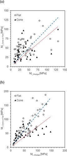
Table 3. Slope and coefficient of determination for two different drop heights.

	Cone		Flat
	5 cm	50 cm	5 cm	50 cm
Slope	0.82	0.74	1.00	1.20
Coefficient of determination	0.669	0.751	0.754	0.923

Correlations

Figure 13 compares the resilient moduli estimated using the IMD with LWD and shear moduli. The linear relationships between the resilient, LWD, and shear moduli are established as follows: (10) $E_{LWD}=a\cdot M_{r\mathrm{\_}IMD}+b$(10) (11) $G_{max}=c\cdot M_{r\mathrm{\_}IMD}+d$(11) where a and b denote the slope of the line and intercept for the linear relationship between the resilient and LWD moduli, respectively; and c and d are the slope of the line and intercept for the linear relationships between the resilient and shear moduli, respectively. The values of the slope and intercept are summarised in Table 4. Figure 13(a) shows the relationships between the resilient and LWD moduli. Regardless of the hammer drop height, the resilient modulus was higher than the LWD modulus. However, higher drop heights resulted in lower slopes and higher R² values for the linear relationships between the resilient and LWD moduli. Figure 13(b) shows the relationships between the resilient and shear moduli. For the hammer drop height of 5 cm, the resilient modulus was smaller than the shear modulus; whereas, for hammer drop height of 50 cm, the resilient modulus was greater than the shear modulus. The R² for the relationship between the shear and resilient moduli was greater for a hammer drop height of 50 cm than for a hammer drop height of 5 cm. Thus, high hammer drop heights may be adequate for estimating resilient moduli using the IMD.

Figure 13. Relationship between the resilient modulus and (a) LWD modulus and (b) shear modulus. Blue and red lines indicate the linear relationships for hammer drop heights of 5 and 50 cm, respectively.

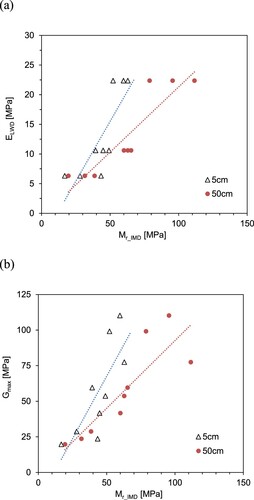
Table 4. Summary of linear relationships of resilient modulus, E_LWD and G_max.

	ELWD		Gmax
	5 cm	50 cm	5 cm	50 cm
Slope of line	0.403	0.220	1.76	0.951
Intercept	–4.65	–0.684	–20.3	–2.46
Coefficient of determination	0.670	0.835	0.616	0.754

The boundary conditions of the laboratory-compacted specimens were different from those of field tests. Therefore, the resilient moduli obtained using the IMD presented in this study may differ from those obtained from field tests using the IMD. Given that the resilient modulus of subgrade is primarily affected by factors, including applied stress, water content, and dry density of soils, a more comprehensive study is needed to establish the relationships between the resilient moduli estimated from the repeated load triaxial test and field tests using the IMD under the same soil conditions.

Conclusions

In this study, various factors affecting resilient modulus estimation using IMD were investigated. In particular, flat, wedge, and cone tips of IMD were designed to compare their performance. Furthermore, the specimens were compacted with three different water contents, and the hammer drop height varied between 5 and 50 cm. Dynamic penetration tests using the IMD were conducted with various factors to compare the maximum force, recoverable displacement, and resilient modulus of the specimens. The maximum shear modulus, Poisson’s ratio, and LWD modulus of the specimens were estimated using bender and piezo-disk elements, and LWD, respectively. Finally, the relationships between the IMD, shear, and LWD moduli were compared. The following conclusions can be drawn based on the obtained results.

• The resilient modulus, based on maximum force and recoverable displacement, increased with penetration depth, and the increase was greater at lower water content. As the water content increased, the maximum shear modulus decreased and the Poisson’s ratio increased. Additionally, E_LWD decreased as water content increased, owing to a decrease in the dry density of the compacted soils.

• Regardless of the tip shape, the resilient modulus for the hammer drop height of 50 cm was greater than that for the hammer drop height of 5 cm. At low resilient modulus ranges, the hammer drop height had less of an effect on the resilient modulus. Overall, the relationship between the resilient moduli for a drop height of 50 cm exhibited a higher R² value than that at a hammer drop height of 5 cm.

• The linear relationship between the resilient moduli for the flat and wedge tips had a slope of one, whereas the resilient modulus for the cone tip was lower than that for the wedge tip. In addition, regardless of the hammer drop height, the R² for the relationship between the flat and wedge tips was greater than that between the cone and wedge tips.

• There is a linear relationship between the resilient, LWD, and shear moduli. In particular, higher hammer drop heights resulted in a lower slope and a higher R² value of the correlations. Therefore, high hammer drop heights are required for resilient modulus estimation using IMD.

Disclosure statement

No potential conflict of interest was reported by the author(s).

Additional information

Funding

This work was supported by the National Research Foundation of Korea (NRF) grant funded by the Korean government (MSIT) (No. NRF-2021R1A5A1032433).

References

- AASHTO, 2008. Mechanistic-empirical pavement design guide: A manual of practice. Washington, DC, USA.
- AASHTO M., 2004. Standard specification for materials for aggregate and soil-aggregate subbase, base, and surface courses.
- ASTM, D., 2012. Standard test methods for laboratory compaction characteristics of soil using modified effort, ASTM D698.
- Byun, Y.H., et al., 2018. Embedded shear wave transducer for estimating stress and modulus of As-constructed unbound aggregate base layer. Construction and Building Materials, 183, 465–471.
- Byun, Y.H., and Kim, D.J, 2022. In-situ modulus detector for subgrade characterization. International Journal Pavement Engineering, 23 (2), 297–307.
- Byun, Y.H., and Lee, J.S, 2013. Instrumented dynamic cone penetrometer corrected with transferred energy into a cone tip: a laboratory study. Geotechnical Testing Journal, 36 (4), 533–542.
- Duddu, S.R., and Chennarapu, H, 2022. Quality control of compaction with lightweight deflectometer (LWD) device: a state-of-art. International Journal of Geo-Engineering, 13 (1), 1–13.
- Gabr, M.A., et al., 2000. DCP criteria for performance evaluation of pavement layers. Journal of Performance of Constructed Facilities, 14 (4), 141–148.
- Hong, W.T., et al., 2017. Strength and stiffness assessment of railway track substructures using crosshole-type dynamic cone penetrometer. Soil Dynamics and Earthquake Engineering, 100, 88–97.
- Hong, W.T., Kim, S.Y., and Lee, J.S, 2022. Evaluation of driving energy transferred to split spoon sampler for accuracy improvement of standard penetration test. Measurement, 188, 110384.
- Jibon, M., and Mishra, D, 2021. Light weight deflectometer testing in Proctor molds to establish resilient modulus properties of fine-grained soils. Journal of Materials in Civil Engineering, 33 (2), 06020025.
- Kim, K., et al., 2008. Effect of penetration rate on cone penetration resistance in saturated clayey soils. Journal of Geotechnical and Geoenvironmental Engineering, 134 (8), 1142–1153.
- Kim, D.J., and Byun, Y. H, 2019. Development and performance evaluation of in-situ dynamic stiffness analyzer. Journal of The Korean Society of Agricultural Engineers, 61 (2), 41–50.
- Kim, S.Y., and Lee, J.S, 2020. Energy correction of dynamic cone penetration index for reliable evaluation of shear strength in frozen sand–silt mixtures. Acta Geotechnica, 15 (4), 947–961.
- Kim, D.J., Yu, J.D., and Byun, Y.H, 2021. Piezoelectric ring bender for characterization of shear waves in compacted sandy soils. Sensors, 21 (4), 1226.
- Kleyn, E.G., 1975. The use of the dynamic cone penetrometer (DCP), Transvaal Roads Department, Report Number L2/74, Pretoria.
- Langton, D.D., 1999. The Panda lightweight penetrometer for soil investigation and monitoring material compaction, Ground Engineering.
- Lee, J.S., et al., 2019. Assessing subgrade strength using an instrumented dynamic cone penetrometer. Soils and Foundations, 59 (4), 930–941.
- Li, C., et al., 2018. In situ modulus reduction characteristics of stabilized pavement foundations by multichannel analysis of surface waves and falling weight deflectometer tests. Construction and Building Materials, 188, 809–819.
- Livneh, M., Ishai, I., and Livneh, N.A, 1992. Automated DCP device versus manual DCP device. Road Transport Research, 1 (4), 48–61.
- Nazzal, M., et al., 2004. Evaluating the potential use of a portable LFWD for characterizing pavement layers and subgrades. Geotechnical Engineering for Transportation Projects, 1, 915–924.
- Peraka, N.S.P., and Biligiri, K.P, 2020. Pavement asset management systems and technologies: A review. Automation in Construction, 119, 103336.
- Schmertmann, J.H., Hartman, J.P., and Brown, P.R, 1978. Improved strain influence factor diagrams. Journal of Geotechical Engineerig Division, 104 (8), 1131–1135.
- Schwartz, C.W., Afsharikia, Z., and Khosravifar, S, 2017. Standardizing lightweight deflectometer modulus measurements for compaction quality assurance (No. MD-17-SHA-UM-3-20). Maryland. State Highway Administration.
- Tovar-Valencia, R.D., et al., 2021. Effect of base geometry on the resistance of model piles in sand. Journal of Geotechical and Geoenvironmental Engineering, 147 (3), 04020180.
- Umashankar, B., Hariprasad, C., and Kumar, G.T, 2016. Compaction quality control of pavement layers using LWD. Journal of Materials in Civil Engineering, 28 (2), 04015111.
- Webster, S.L., Grau, R.H., and Williams, T.P., 1992. Description and application of dual mass dynamic cone penetrometer, Instruction Report GL-92-3, Department of the Army, US Army Corporation of Engineers, Washington, DC.
- Xu, Q., and Chang, G.K, 2013. Evaluation of intelligent compaction for asphalt materials. Automation in Construction, 30, 104–112.