Gravel road classification based on loose gravel using transfer learning

ABSTRACT

Road maintenance agencies subjectively assess loose gravel as one of the parameters for determining gravel road conditions. This study aims to evaluate the performance of deep learning-based pre-trained networks in rating gravel road images according to classical methods as done by human experts. The dataset consists of images of gravel roads extracted from self-recorded videos and images extracted from Google Street View. The images were labelled manually, referring to the standard images as ground truth defined by the Road Maintenance Agency in Sweden (Trafikverket). The dataset was then partitioned in a ratio of 60:40 for training and testing. Various pre-trained models for computer vision tasks, namely Resnet18, Resnet50, Alexnet, DenseNet121, DenseNet201, and VGG-16, were used in the present study. The last few layers of these models were replaced to accommodate new image categories for our application. All the models performed well, with an accuracy of over 92%. The results reveal that the pre-trained VGG-16 with transfer learning exhibited the best performance in terms of accuracy and F1-score compared to other proposed models.

KEYWORDS:

• Convolutional neural networks
• transfer learning
• deep learning
• loose gravel
• gravel road maintenance
• road condition assessment

1. Introduction

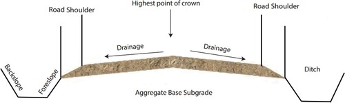
Gravel roads connect areas of sparse populations and provide pathways for agricultural and forest goods. Gravel roads are also considered where the traffic volume is low, where gravel roads are more economical in comparison to paved roads. In Sweden, 21% of the public roads are gravel roads owned by the state, covering over 20 200 km. Besides, 74 000 km of gravel roads and forest roads of 210 000 km exist owned by the private sector (Kans et al. 2020, Saeed et al. 2020). The Swedish Road Administration (Trafikverket) rates the gravel road condition according to the severity of irregularities (corrugation and potholes), dust, and loose and gravel cross-section (Alzubaidi 2001). This assessment is done during the summertime when roads are free of snow (Hossein Alzubaidi 2014). Similar road distresses can be considered in other countries when assessing the quality of gravel roads. Gravel roads are made up of layers of soil and aggregates. In Figure 1, the structure of a gravel road is shown. The durability of gravel roads is low and requires regular maintenance. Some approaches are used to improve the safety of gravel roads using environment-friendly, cost-effective, and sustainable solutions. These solutions include a well-compacted road surface, a surface seal that creates a hard water resistance surface, and well-planned maintenance activities (Albatayneh et al. 2019).

Figure 1. Cross-section structure of gravel.

There are various visual gravel road assessment methods used worldwide that are regulated by the country’s weather and landscape. Previous studies have shown that visual assessments are unreliable (Nyberg et al. 2015, Nyberg, 2016). There can be a difference in rating the same road by various experts. The manual classification of loose gravel is tiresome and dangerous for the people involved. Therefore, many road management agencies are shifting to objective, efficient, cost-effective technological solutions.

Several smartphone applications are available that are capable of road profiling, such as RoadRoid, RoadSense, etc. (Forslöf and Jones 2015, Allouch et al. 2017). These applications use smartphone accelerometers to collect data and give an overall picture of the road by calculating the international roughness index (IRI). The IRI obtained from these applications helps quantify general road roughness. These applications are cost-effective, but their limitation is that nothing can be inferred about the type of distress causing the road roughness. Applications that could give more information about the distress type would benefit road maintenance agencies.

In 2017, around 600 people died in the United States in accidents on gravel roads. Most of these accidents were multiple-vehicle crashes. The hazardous defects include too much loose gravel, dust impairing visibility, and lack of traffic signs (Albatayneh et al. 2020). Gravel roads become slippery when the surface contains excessive loose aggregate with fine aggregate within the crust (Nervis and Nuñez 2019). Loose gravel can slip under vehicle tires and cause drivers to lose control when slamming on the brakes or abruptly diverging while driving on gravel roads (Kanhere 2011). This shows how critical it is to keep loose gravel conditions monitored and maintained timely, not only for a comfortable ride but also for the safety of the drivers. In this study, one of the artificial intelligence (A.I) application is developed to automatically classify gravel roads according to the severity of loose gravel on gravel roads in accordance with the rating scale suggested by the Swedish Road Administration authority. Such detection using A.I can be considered an innovative method to help road maintenance agencies by quantifying the presence of loose gravel. This paper used a transfer learning technique to retrain several pre-train models. VGG-16 is proposed to classify loose gravel on gravel roads into two major categories.

The rest of this article is organised as follows: first, the literature review covering related studies is presented. Then the methodology is presented, discussing data collection and the dataset, pre-processing of data, transfer learning, CNN, discriminative learning, and evaluation metrics used in this study, followed by results and discussion. The article ends with concluding remarks and references.

2. Literature review

This section will discuss classical road evaluation methods and studies involving image analysis for road defect detection. The literature mainly concerns conventional gravel road maintenance methods. Some research studies have been conducted using automated machine learning approaches for identifying road defects. Most of these studies focus more on paved roads and less on unpaved roads (Abulizi et al. 2016, Allouch et al. 2017, Gorges et al. 2019). There are fewer studies about gravel road distress identification using artificial intelligence. Therefore, some studies on paved road defects will also be included here.

For gravel road condition assessment in Sweden, the regulation Gravel Road Assessment (Bedömning av grusväglag) is laid down by the Swedish Transport Administration (Trafikverket). According to this method, the evaluation of gravel road defects is primarily assessed visually by human inspectors. Only the conditions of cross fall and road edges are objectively evaluated against the threshold for each class. This objective measurement is not complex and is done by simple tools, such as a cross-fall metre or a digital metre measuring the cross-fall (Alzubaidi 1999). Images of the gravel roads are taken by driving through gravel roads and are accessed by the experts, comparing them with some standard condition pictures. Rating for each road helps decision-makers decide whether a gravel road needs maintenance. Details of the method can be found in the following reference document by Trafikverket (Karin Edvardsson, Thomas Lundberg 2015).

Similar visual gravel road assessment methods are used worldwide. The country’s weather and landscape regulate them. In some cases, statistical data is collected from vehicles fitted with specialised instruments that take road surface measurements. For instance, a laser profiler in Sweden, an Automated Road Analyzer (ARAN) used in Canada, and a Road Measurement Data Acquisition system (ROMDAS) are used in New Zealand for road assessment (Hossein Alzubaidi 2014, Saeed et al. 2020), (Sodikov et al. 2005). These complex trucks are costly and cannot be used for gravel roads, as one of the goals of having gravel roads is to keep these pathways economical. Moreover, road roughness surveys can provide valuable overall road conditions concerning the driver’s comfort. But the surveys do not reflect adequate information to identify a particular distress type’s existence and intensity (Nervis and Nuñez 2019).

Applications, such as Roadroid and Roadsense, are available for smartphones; these applications calculate the overall road roughness index and map road conditions on maps. These applications cannot help identify the type of distress present (Forslöf and Jones 2015, Allouch et al. 2017). As discussed earlier, conventional automated objective road assessment methods are quite expensive. Therefore, the role of technology is essential to minimise subjective measurement and provide cost-effective, efficient distress evaluation, productivity, and repeatability.

Past studies show that road defects such as dust, rutting, wash boarding, or potholes can be identified by applying machine vision techniques to images and video data. Changes in colour or texture in these patterns indicate the loss of aggregate from the road surface (Nervis and Nuñez 2019, Rajab et al. 2008, Gopalakrishnan et al. 2017, C. Zhang and Elaksher 2012). In 2003, Patric et al. (Patrick and Foedisch 2003) used colour-based segmentation to determine the road type as asphalt, dirt, snow, or gravel-surfaced road. Support vector machines (SVM) have been compared with artificial neural networks. SVM performed slightly better than neural networks, but this difference has been insignificant. Image coordinates have also been added as an additional feature for model training to minimise the misclassification of the road as background. Identifying paved roads through machine vision algorithms can be easily done as the lane is adequately marked. Conversely, dirt or gravel roads are hard to identify as they do not have clear markings. These roads merge with their surrounding environment during the snow or rain.

In 2012, Cord et al. (Cord and Chambon 2012) presented a method of automatically distinguishing defects on paved roads, such as grabbing holes and cracks. The process was based on supervised learning, using AdaBoost. The VisTex image database and on-road images collected by a dedicated road imaging system were used. The textural information was described by a large set of linear and non-linear filters.

In 2012, Zang et al. (C. Zhang and Elaksher 2012) presented a semi-automated method that utilised images of ruts on gravel roads by unmanned Aerial Vehicle (UAV) drone. Two images captured from two different viewpoints are analysed to derive the 3D information of the identified and matched feature points; hence the system is stereo in effect, although it has a monocular vision at any given point in time. Acquired images were converted to 3D images to measure the depths of these ruts. The reconstruction process is helped by the relative displacement of the UAV calculated by two onboard sensors: a Global Positioning System (GPS) sensor and an inertial measurement unit. The results were quite close to manual measurements, but the method’s high complexity is difficult to implement.

In 2019, Albatayneh et al. (Albatayneh et al. 2019) proposed a simple dust classification algorithm using images taken from a smartphone application, ‘Roadroid,’ to classify the amount of dust using proprietary digital Image Processing algorithms. A Dustometer device was used to validate the proposed algorithm. Dustometer measurements, supported by statistical analysis, demonstrate that the proposed algorithm achieves outstanding classification accuracy.

In 2021, Albatayneh et al. (Abu Daoud et al. 2021) validated the practicality of a deep learning-based image classifier trained to classify gravel road images according to the severity level of corrugations present on the gravel road. Furthermore, the classifier was tested to check applicability in practice. Images were collected from gravel roads in Laramie County, Wyoming. Corrugation images were evaluated by visual inspection methods and by the developed classifier. A confusion matrix showed that the classifier had an accuracy of 83% in the practical field. According to the study, the achieved accuracy level is sufficient for the Gravel Roads Management Systems (GRMS) followed in the USA.

The literature review shows that much research has been dedicated mainly to overall road roughness and less to identifying distress types for gravel roads. Moreover, addressing the automation of measuring loose aggregate seems ignored (Gopalakrishnan et al. 2017, Mednis et al. 2011, Rajab et al. 2008, Wang et al. 2015).

3. Materials and methods

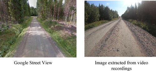
This study’s data consists of gravel road images collected from two sources. The first data source was created by extracting images from recorded videos while driving on gravel roads at 50 km/hr around Dalarna County, Sweden. Two GoPro HERO7 cameras were used. One of the cameras was fixed to the windshield inside. The other was outside on the vehicle’s bonnet with a double clip strong suction cup to keep the camera steady without obscuring the camera lens. More details of the data collection can be found in (Saeed et al. 2021). Images from the camera outside were extracted as they had a better view of the road condition. The second source was the images of gravel roads from Google Street View (Anguelov et al. 2010). These images were from gravel roads around Sweden. Although traversing gravel roads on Google Maps and extracting images from Google Street View is quite time-consuming, Google Street View could be used for many image analysis problems. Multiple data sources were used to increase the size of the data set, generalisation, and diversity for the model to learn. A data set of 638 images was collected, combining the images from two cameras and Google Street View. Some of the images of gravel roads are shown in Figure 2.

Figure 2. Example images from various sources included in the data set.

3.1. Pre-processing data

For this study, 638 images were labelled by the first author in two classes: 1 & 2 ratings, and 3 & 4 ratings, as shown in Figure 3. These classes or categories represent images according to road condition grading by Trafikverket (Hossein Alzubaidi 2014). Due to the limited size of the image data set, images are not categorised into four classes. Categories 1&2 and 3&4 are quite similar; therefore, images of roads with conditions identical to ratings 1 and 2 were combined as one class, named ratings 1 & 2. And roads with conditions comparable to ratings 3 and 4 were also incorporated as another class, called ratings 3&4. This labelling was done by referring to ground truth images present in the Trafikverket standard images of ratings 1, 2, 3, and 4 in its manual (Hossein Alzubaidi 2014). This classification can help road maintenance agencies identify roads of good quality or bad quality and create maintenance plans accordingly. As the images in the data set came from various sources, pixel intensity and dimension are not the same across all the images. Normalisation was carried out using ImageNet’s mean and standard deviation to make model training stable and reduce bias. Normalising the data is an important step that makes model training stable and fast. All images were also resized to 224 × 224-pixel size. The most essential pre-processing was to centre crop the image so that the road stays in each image; otherwise, some images might get resized where one can only see a tree, grass, or side of the road. Data augmentation techniques were applied to the data set of 638, such as random horizontal flip, random rotation, and resize. After each augmentation technique is applied, a new set of images is created to be submitted to CNN, thus increasing the data set by three folds after augmentation. Data were split into train and test sets of 60% and 40%, respectively. Table I shows the details of the data set and distribution of the images into classes.

Figure 3. Labelled images used for training CNN.

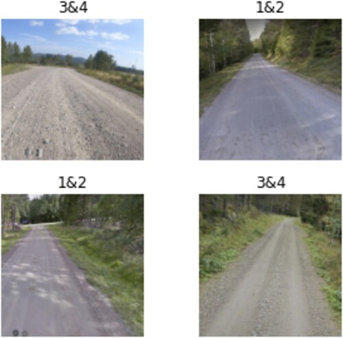
Table I. Details of the data set and class distributions.

Classes	Number of training images	Number of testing images	Total images in each class	Total Images in the dataset
1&2	163	109	272
3&4	220	146	366	638

3.2. Retraining a deep neural network (Transfer learning)

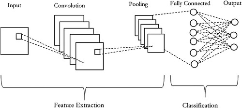
In practice, as it is not common to have a dataset of sufficient size, it is unusual to train an entire convolution network from scratch with random initialisation of weights. In the case of small datasets, it has been shown that transfer learning can be useful (Transfer learning for computer vison tutorial n.d.), (Weiss et al. 2016). Transfer learning is an in-depth learning approach that exploits the idea of transfer of knowledge from a pre-trained network trained on large data. Pre-trained models usually help in better initialisation and convergence when the data set is small. Pre-trained networks are trained on the ImageNet data set containing 1.2 million images of 1000 categories to another image classification task with a relatively smaller data set, such as knowledge gained for recognising cars can detect trucks in another problem (George Karimpanal and Bouffanais 2019, Russakovsky et al. 2015). Using transfer learning avoids training a network from scratch, which may take extensive computing power and training for days or weeks on Graphics Processor Unit (GPU). Generalised features learned by the earlier layers of the pre-trained networks, such as blobs, edges, colours, etc., can help a comparatively different computer vision problem. Figure 4 shows a typical CNN topology.

Figure 4. A typical CNN Architecture.

3.3. Discriminative learning

In this study, discriminative learning, also called cyclic learning, is used to determine the optimal learning rate for training layers of pre-trained CNN models. The learning rate is a hyperparameter that controls the speed at which the model learns. The weights are scaled by learning rate to minimise the loss. A lower learning rate might be a good way to avoid missing optimal solutions. At the same time, it could also mean that it will take more time to converge. Discriminative fine-tuning was introduced by Jeremy Howard and Sebastian Ruder (Howard and Ruder 2018). Their proposed method is that when different layers in a CNN capture different information, layers should be fine-tuned to different extents (Howard and Ruder 2018). Instead of using the conventional practice of increasing or decreasing learning rates, the model layers are grouped. The earlier layers can recognise general details such as lines, curves etc. These initial layers are helpful in most of the tasks. These layers are trained at a lower learning rate so that the model has more time to train on small details. Hence, the later layers are more task-specific and not useful, such as for gravel road condition classification. These later layers are therefore trained at a higher rate. This way, the weights of lower rates will be changed less than the later layers (Mushtaq et al. 2021, F. Zhang et al. 2021). The first phase layers, before the newly added classification layer, are frozen since they are already well trained; this will keep the weight unchanged during the training. In the second phase, all the layers are unfrozen and trained.

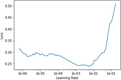
The optimal rate range can be found with the benefit of a learning rate finder from the Fastai library [35]. Fastai library is a deep learning library based on top of PyTorch. Pytorch is an open-source machine learning framework based on python (Paszke et al. 2019). Figure 5 shows the output of a discriminative learning rate finder. It shows a relation between the learning rate and loss over each iteration. It can be seen that the loss function increases or decreases with respect to the learning rate. It can be seen in the below graph where the loss is getting constantly lower; in this case, it follows a steep path from 1e⁻⁰⁴ to 1e⁻⁰³. This is the optimal learning rate in this case. The earlier layers will be trained at a lower learning rate of le⁻⁰⁴ and the higher layers of le⁻⁰³. After this range, it is seen that the loss function stops decreasing and then increases. The idea is to choose a range where the loss function continues to decline.

Figure 5. Learning rate finder.

3.4. Pre-trained CNN

The methodology followed in this study is shown in Figure 6. Six pre-trained networks, including their variants, were used in this study. These are briefly discussed as follows:

Figure 6. Workflow of the proposed approach for detecting loose gravel.

3.4.1. Residual network (Resnet)

In this study, two variants of ResNet are used, namely ResNet18 and ResNet50. ResNet50 is a residual network having 50 layers, whereas ResNet18 has 18 layers. It is similar to VGG-16, except that Resnet50 has a supplementary identity mapping capability. ResNet reduces the vanishing gradient problem by an alternate shortcut path. This skipping effectively simplifies the network, using fewer layers in the initial training stage, where identity mapping allows the model to converge faster by optimising the backpropagation path. Identity mapping helps in avoiding overfitting (Dhananjay Theckedath 2020).

3.4.2. Alexnet

Alexnet used a non-saturating Rectified Linear Units (ReLU) activation function instead of Tanh activation and sigmoid. Using ReLU showed improvement in Training performance. It also introduced the concept of dropout. Dropout is used to reduce overfitting in fully connected layers. It is a technique for turning off neurons with a predetermined probability. With each iteration, the model uses different parameters that enable each neuron to have robust features that can be used with other random neurons. However, this method increases the training time needed for CNN to converge, which was made feasible using a multi-graphics processing unit (GPU) (Krizhevsky et al. 2012).

3.4.3. Densenet

DenseNet introduced the concept of dense connections between layers through Dense blocks, where all layers connect with matching feature-map sizes directly to each other. This connectivity pattern yields state-of-the-art accuracies on CIFAR10/100 (with or without data augmentation) and the street view house numbers (SVHN) Data sets. DenseNets have several compelling advantages: they alleviate the vanishing gradient problem, strengthen feature propagation, encourage feature reuse, and significantly reduce the number of parameters. Using less than half the number of parameters on the ILSVRC 2012 (ImageNet) dataset, DenseNet achieves similar accuracy to ResNet (Iandola et al. 2014).

3.4.4. Visual geometry group (VVG 16)

Oxford University proposed the VGG model, one of the most influential models that reinforced the notion that making the architecture or CNN deeper improves performance. Its main contribution is using a deeper convolution network with small 3 × 3 convolutional filters. The performance improved based on increasing the depth from 16 to 19 layers. Their findings were proved in model submission in Image challenge 2015, where the VGG model secured first and second place in localisation and classification tracks, respectively., although numerous follow-up works improved VGG architecture (Hameed et al. 2020, Simonyan and Zisserman 2016). For this study, VGG16, is used, which contains 16 weight layers.

3.5. Evaluation metrics

In this study, several metrics were used to evaluate the performance of classifier metrics, such as accuracy, F1-score, recall, and precision. These metrics are widely used to measure classifier performance. Accuracy is defined as the percentage of testing data correctly classified. In classification with imbalanced data, looking at other metrics, such as precision, recall, and F1-score, can provide essential insights. Intuitively, the class with more examples will have more chances of being classified better, and hence the model’s overall performance might be good.

Nevertheless, looking at how well the negative class is classified is required. F1-score is the mean of precision and recall. TP (True Positive) is correctly classified as instances of the true class, and TN (True Negative) is correctly classified as instances of the negative class.

Similarly, False Positive (FP) and False Negative (FN) mean incorrectly classified true and negative class instances, respectively (Wardhani et al. 2019, Hameed et al. 2020). In classification problems with imbalanced data, the class with more examples, or the majority class, is considered a negative class. The class with fewer examples is regarded as a positive class, so classes 1&2 are the positive class in this case. These performance metrics can be calculated as follows:

• Accuracy evaluates the correctness of the model and its ratio of correctly classified images to the total number of testing images $Accuracy={\displaystyle \frac{TP+TN}{TP+TN+FP+FN}}$

• Precision quantifies the exactness of a model and represents the ratio of images from classes 1&2 correctly classified out of the union of the predicted same class. $Precision={\displaystyle \frac{TP}{TP+FP}}$

• Recall is also called sensitivity; it is the completeness of a model. It computes the ratio of images correctly classified as classes 1&2 out of the total number of images of true class. $Recall={\displaystyle \frac{TP}{TP+FN}}$

• F1-score represents the harmonic average of precision and recall and is usually used to optimise a model towards either precision or recall. This metric is the most-used member of the parametric family of the F-measures, named after the parameter value β = 1. F1 score is defined as the harmonic mean of precision and recall (Chicco and Jurman 2020). $F1={\displaystyle \frac{2.TP}{2.TP+FP+FN}.2.{\displaystyle \frac{Precision.Recall}{Precision+Recall}}}$

• The error rate is the proportion of instances misclassified. Accuracy and error rate complement each other. $Error={\displaystyle \frac{FP+FN}{TP+TN+FN+FP}}$

4. Results

All the models (AlexNet, ResNet18, ResNet50, DesnseNet121, DenseNet201, and VGG16) were trained using the standard two-phase training discussed in section 3.3. The results show gravel road classification with deep learning can be achieved with decent accuracy with a small and imbalanced dataset. The metrics for each model with other details, such as training and validation loss, error rate, number of epochs, and the learning rate for each phase, are presented in Table II. All the models have performed well on our data set, with an accuracy of over 92%. The findings shown in Table II indicate that the pre-trained Vgg16 model with transfer learning outperforms other models. The recall of Vgg16 is the highest, which means there are more positive class cases classified or detected by Vgg16 than in the rest of the models. The positive class here is class 1&2 having fewer examples. Although in it might seem that it would be more interesting to only get class 3&4 of gravel to be classified correctly as these roads are in critical need of maintenance. Correct classification of the minority class 1&2 (roads with good and fair gravel road conditions) also means that they will not be misclassified as gravel roads of categories 3&4 (Bad and worst) gravel road conditions. Hence the performance of CNN is reassuring. Vgg16 also has the highest accuracy but is similar to ResNet50. Vgg16 outperforms by having the highest F1-score, which is the harmonic mean of precision and recall, which is a better indicator of the model’s overall performance regarding imbalanced data. Similarly, the performance of Densnet201 is also commendable, with accuracy and F1-score close enough to Vgg16, with a difference of only 1%. Training and validation loss are also monitored to avoid overfitting.

Table II. Performance results of pre-trained networks.

Network	Training loss	Validation loss	Accuracy	Error rate	Precision	Recall	F1 Score	Epochs phase 1	Epochs phase 2	Learning rate range phase1	Learning rate range phase 2
ResNet18	0.151	0.185	0.922	0.078	0.992	0.867	0.890	5	3	1e-3,1e-2	1e-4,1e-3
ResNet 50	0.220	0.144	0.965	0.035	1.000	0.937	0.949	5	3	1e-3,1e-2	1e-4,1e-3
Alexnet	0.300	0.163	0.941	0.059	0.971	0.923	0.932	5	3	1e-3,1e-2	1e-4,1e-3
Densenet121	0.777	0.204	0.922	0.078	0.936	0.923	0.926	5	3	1e-3,1e-2	1e-5,1e-4
Densenet201	0.138	0.245	0.957	0.043	0.965	0.958	0.959	5	3	1e-3,1e-2	1e-4,1e-3
Vgg16	0.253	0.130	0.961	0.039	0.965	0.965	0.965	5	3	1e-3,1e-2	1e-4,1e-3

5. Discussion

The experimental results show that state-of-the-art, pre-trained CNN architectures using transfer learning can classify images according to the loose gravel condition of the road with appreciable accuracy. A data set of 638 images showing loose gravel conditions on gravel roads has been used. These images were obtained while driving through gravel roads of Dalarna County, Sweden. The data set was increased by three folds by using augmentation techniques. Results show that Vgg16 performed better with consistent accuracy of 96% and an F1-score of 0.96. Vgg16 performs highest in classifying loose gravel conditions in both positive classes (1&2) and negative classes (3&4). The findings of this paper provide a solid basis to advance the use of transfer learning through pre-trained CNN models used for gravel road condition classification through images.

One question might arise about how the proposed system would react when classifying input-given images with variations in colour intensities. An algorithm was developed to convert the images to greyscale images and train the CNN network to test the sensitivity of the proposed model. For this experiment, only Vgg16 was retrained as it was selected as it outperformed previously. Vgg16 classified greyscale images with an accuracy of 0.94, precision of 0.934, recall of 0.975, and F1-score of 0.954. Converting images to greyscale would bring all images to a standard colour model. This method would make the system independent of the colour schemes of the input images. The results were quite similar to the previous experiments.

The advantages of using pre-trained CNN models with transfer learning for classification are manifold: firstly, the classification mechanism is fully automated.

Secondly, it removes the conventional steps of segmentation, region of interest (ROI) outlining, feature extraction, and selection. Thirdly, no inter-and intra-observer biases are there during the classification, and the predictions made by the pre-trained CNN models are reproducible with a high accuracy.

6. Conclusion

Data were obtained by driving and recording videos through Dalarna County, Sweden. Also, some images were added from Google Maps, traversing the gravel roads of Sweden. All the data represented Swedish gravel roads. Therefore, this method could be applied to gravel roads in Sweden and countries with similar terrain and climate. These automated solutions using the proposed method can relieve much of the burden on human experts by providing cost-effective, efficient, and reliable assessments. They can replace traditional visual inspection and automated methods requiring sophisticated and expensive equipment. The research outcomes provide practical guidelines for developing transfer-learning-based solutions for gravel road condition assessment methods.

In the future, experiments will be executed on the pre-trained networks with more training data to classify images into four classes, as suggested by Trafikverket. An additional class with invalid images that don’t need classification could be added, such as images with cars, etc. In this study, the first author carried out the labelling of images. For a better interpretation of important features learned by CNN for making classification decisions, algorithms such as Gradient-weighted Class Activation Mapping (Grad-cam) and guided propagation be used in future work. This helps in the interpretability of the model. It would be interesting to have the classification done by experts from Trafikverket. Furthermore, it would also be interesting to study human inter-rater variability in the condition-wise manual classification of gravel road images.

Disclosure statement

No potential conflict of interest was reported by the author(s).

References

- Abu Daoud, O., et al., 2021. Validating the practicality of utilising an image classifier developed using TensorFlow framework in collecting corrugation data from gravel roads. International Journal of Pavement Engineering, May, 1–12. doi:10.1080/10298436.2021.1921773
- Abulizi, N., et al., 2016. Measuring and evaluating of road roughness conditions with a compact road profiler and ArcGIS. Journal of Traffic and Transportation Engineering (English Edition), 3 (5), 398–411. doi:10.1016/j.jtte.2016.09.004.
- Albatayneh, O., et al., 2020. Complementary modeling of gravel road traffic-generated dust levels using Bayesian regularization feedforward neural networks and binary probit regression. International Journal of Pavement Research and Technology, 13 (3), 255–262. doi:10.1007/s42947-020-0261-3.
- Albatayneh, O., Forslöf, L., and Ksaibati, K., 2019. Developing and validating an image processing algorithm for evaluating gravel road dust. International Journal of Pavement Research and Technology, 12 (3), 288–296. doi:10.1007/s42947-019-0035-y.
- Allouch, A., et al., 2017. Roadsense: smartphone application to estimate road conditions using accelerometer and gyroscope. IEEE Sensors Journal, 17 (13), 4231–4238. doi:10.1109/JSEN.2017.2702739.
- Alzubaidi, H., 1999. Operation and maintenance of gravel roads: A literature study. http://www.diva-portal.org/smash/record.jsf?pid=diva2%3A673330&dswid=−4629.
- Alzubaidi, H., 2001. On rating of gravel roads. PhD dissertation. KTH.
- Anguelov, D., et al., 2010. Google street view: capturing the world at street level. Computer, 43 (6), 32–38. doi:10.1109/MC.2010.170.
- Chicco, D. and Jurman, G., 2020. The advantages of the Matthews correlation coefficient (MCC) over F1 score and accuracy in binary classification evaluation. BMC Genomics, 21 (1), 6. doi:10.1186/s12864-019-6413-7.
- Cord, A. and Chambon, S., 2012. Automatic road defect detection by textural pattern recognition based on AdaBoost. Computer-Aided Civil and Infrastructure Engineering, 27 (4), 244–259. doi:10.1111/j.1467-8667.2011.00736.x.
- Dhananjay Theckedath, R.R.S., 2020. Detecting affect states using VGG16, ResNet50 and SE-ResNet50 networks. SN Computer Science. doi:10.1007/s42979-020-0114-9
- Forslöf, L. and Jones, H., 2015. Roadroid: continuous road condition monitoring with smart phones. Journal of Civil Engineering and Architecture, 9 (4), 485–496. doi:10.17265/1934-7359/2015.04.012.
- George Karimpanal, Thommen and Bouffanais, R., 2019. Self-organizing maps for storage and transfer of knowledge in reinforcement learning. Adaptive Behavior, 27 (2), 111–126.
- Gopalakrishnan, K., et al., 2017. Deep Convolutional Neural Networks with transfer learning for computer vision-based data-driven pavement distress detection. Construction and Building Materials, 157, 322–330. doi:10.1016/j.conbuildmat.2017.09.110.
- Gorges, C., Öztürk, K., and Liebich, R., 2019. Impact detection using a machine learning approach and experimental road roughness classification. Mechanical Systems and Signal Processing, 117, 738–756. doi:10.1016/j.ymssp.2018.07.043.
- Hameed, Z., et al., 2020. Breast cancer histopathology image classification using an ensemble of deep learning models. Sensors, 20 (16), 4373–17. doi:10.3390/s20164373.
- Hossein Alzubaidi, 2014. Bedömning av grusväglag (Assesment of gravel roads),TDOK 2014:0135 Version 1.0, Trafikverket. https://trafikverket.ineko.se/Files/sv-SE/10845/RelatedFiles/2005_060_bedomning_av_grusvaglag.pdf.
- Howard, J. and Ruder, S., 2018. Universal language model fine-tuning for text classification. Acl 2018 – 56th annual meeting of the association for computational linguistics, proceedings of the conference (long papers), 1, 328–339. doi:10.18653/v1/p18-1031
- Iandola, F., et al., 2014. Densenet: Implementing efficient convnet descriptor pyramids. ArXiv Preprint ArXiv:1404.1869.
- Kanhere, S.S., 2011. Participatory sensing: Crowdsourcing data from mobile smartphones in urban spaces. Ieee 12th international conference on mobile data management, 6–9 June, Lulea, Sweden, 3–6. doi:10.1109/MDM.2011.16.
- Kans, M., Campos, J., and Håkansson, L., 2020. Smart innovation, systems and technologies. Advances in Asset Management and Condition Monitoring, 166, 451–461.
- Karin Edvardsson, Thomas Lundberg L. S., 2015. Objektiv mätmetod för tillståndsbedömning av grusväglag, VTI rapport 863 Objektiv.
- Krizhevsky, A., Sutskever, I., and Hinton, G.E., 2012. Imagenet classification with deep convolutional neural networks. Advances in Neural Information Processing Systems, 25.
- Mednis, A., et al., 2011. Real time pothole detection using Android smartphones with accelerometers. International Conference on Distributed Computing in Sensor Systems and Workshops (DCOSS), (June 2014), 1–6. doi:10.1109/DCOSS.2011.5982206
- Mushtaq, Z., Su, S.F., and Tran, Q.V., 2021. Spectral images based environmental sound classification using CNN with meaningful data augmentation. Applied Acoustics, 172, 107581. doi:10.1016/j.apacoust.2020.107581.
- Nervis, L.O. and Nuñez, W.P., 2019. Identification and discussion on distress mechanisms of unsurfaced gravel roads. International Journal of Pavement Research and Technology, 12 (1), 88–96. doi:10.1007/s42947-019-0011-6.
- Nyberg, R.G., 2016. Automating condition monitoring of vegetation on railway trackbeds and embankments. Edinburgh University.
- Nyberg, R.G., Yella, S., and Dougherty, M., 2015. Inter-rater reliability in determining the types of vegetation on railway trackbeds. In Web information systems engineering – WISE 2015: 16th international Conference, Miami, FL, USA. Springer, Cham.
- Paszke, A., et al., 2019. Pytorch: An imperative style, high-performance deep learning library. Advances in Neural Information Processing Systems, 32.
- Patrick, C., and Foedisch, M., 2003. Performance evaluation of color based road detection using neural nets and support vector machine. 32nd applied imagery pattern recognition workshop. doi:10.1109/AIPR.2003.1284265
- Rajab, M.I., Alawi, M.H. and Saif, M.A., 2008. Application of image processing to measure road distresses. WSEAS Transactions on Information Science and Applications, 5 (1), 1–7.
- Russakovsky, Olga, et al., 2015. Imagenet large scale visual recognition challenge. International Journal of Computer Vision, 115 (3), 211–252.
- Saeed, N., et al., 2020. A review of intelligent methods for unpaved roads condition assessment. In: 2020 15th IEEE conference on industrial electronics and applications (ICIEA), May, 79–84.
- Saeed, N., et al., 2021. Classification of the acoustics of loose gravel. Sensors, 21 (14). doi:10.3390/s21144944.
- Simonyan, K. and Zisserman, A., 2016. Very deep convolutional neural networks. ICLR 2015, July, Alessandro Luca Vilardi. https://www.robots.ox.ac.uk/~vgg/research/very_deep/.
- Sodikov, J., Tsunokawa, K., and Ul-Islam, R., 2005. Road survey with ROMDAS system: A study in akita prefecture. Departmental Bulletin Paper, (February), 149–151.
- Transfer learning for computer vison tutorial, n.d. https://pytorch.org/tutorials/beginner/transfer_learning_tutorial.html#convnet-as-fixed-feature-extractor.
- Wang, H. W., et al., 2015. A real-time pothole detection approach for intelligent transportation system. Mathematical Problems in Engineering.
- Wardhani, N.W.S., et al., 2019. Cross-validation metrics for evaluating classification performance on imbalanced data. In: 2019 international conference on computer, control, informatics and Its applications: emerging trends in Big data and artificial intelligence, IC3INA 2019, 14–18. doi:10.1109/IC3INA48034.2019.8949568
- Weiss, K., Khoshgoftaar, T.M., and Wang, D., 2016. A survey of transfer learning. Journal of Big Data, 3 (1), 9. doi:10.1186/s40537-016-0043-6.
- Zhang, C. and Elaksher, A., 2012. An unmanned aerial vehicle-based imaging system for 3D measurement of unpaved road surface distresses. Computer-Aided Civil and Infrastructure Engineering, 27 (2), 118–129. doi:10.1111/j.1467-8667.2011.00727.x.
- Zhang, F., Bales, C., and Fleyeh, H., 2021. From time series to image analysis: A transfer learning approach for night setback identification of district heating substations. Journal of Building Engineering, 43, 102537.