Influences of bus traffic loading on asphalt concrete rutting

ABSTRACT

Permanent deformation is the primary failure mode for the asphalt concrete (AC) pavement in urban environment. It is mainly caused by a combination of heavy traffic load, low vehicle speed and channelised traffic. A rut prediction model would therefore be a valuable tool for planning maintenance scheduling and selecting an appropriate asphalt material. This study uses the PEDRO (Permanent deformation in asphalt concrete layers for roads) model to evaluate the rutting performance of flexible pavements in dedicated bus lanes and intersections in urban areas. For this purpose, three road sections along a bus lane in Malmö, Sweden, were selected. To achieve this, AC cores from the road sections were tested using a Shear Box Tester to characterise the asphalt mixtures. Traffic data such as axle load, tyre configuration, speed, and lateral wander distribution of vehicles, and climate data were measured for the selected sections. Field measurements were carried out to assess the structural conditions of the pavements and to measure transverse profiles. This study introduced a procedure for the evaluation and local calibration of the PEDRO rutting model. The results revealed that the prediction of the transverse profiles are generally in good agreement with the rut measurements.

KEYWORDS:

• Asphalt concrete
• viscosity
• permanent deformation
• PEDRO
• bus lane
• shear test

Introduction

One of the major distresses affecting flexible pavements is permanent deformation in asphalt concrete (AC) layers, also called flow rutting. Permanent deformation or rutting in asphalt layers often occurs as depressions in the wheel path with upheavals along the sides. This is due to a combination of material densification and shear deformation, and the main factors that affect permanent deformation behaviour are traffic loading, climate factors (especially temperature), the AC mixture properties of the pavement layers, as well as pavement structure and geometry (Sousa et al. 1991, Garba 2002). Rutting may cause difficulties in steering the vehicle with increased risk to road safety through hydroplaning and low friction (Rana and Hossain 2021). Rutting in bituminous layers is one of the main reasons for rehabilitating urban roads, particularly bus lanes and intersection areas (Abdallah and Nazarian, 2011, Hajj et al. 2011, Li et al. 2013). The slow-moving and channelised heavy traffic with frequent acceleration and braking subjects bus lanes and intersections to high-stress levels. The lateral wander of wheel loads on roadways depends on the lane width, vehicle types (distance between vehicle tyres), the existence of road shoulders, traffic speed, drivers’ habits, etc. (Blab and Litzka 1995, Timm and Priest 2005, McGarvey 2016). Rana and Hossain (2021) reported that the narrower wandering of autonomous vehicles significantly shortens pavement fatigue life and increases pavement rutting compared to human-operated traffic. Furthermore, narrow urban streets in combination with high intensity and low-speed traffic contribute to channelised traffic. The channelised traffic shows a significantly lower standard deviation of lateral wander compared to other roads. The lateral distribution of wheel loads is crucial for pavement performance evaluation since not all traffic loads have the same wheel path. The number of load repetitions at a point is also critical for pavement design (Blab and Litzka 1995, Ali et al. 2009, Said et al. 2011, 2013a, 2017, Oscarsson 2011, Erlingsson et al. 2012, Siddharthan et al. 2017). Thus, the influence of the lateral wander of traffic on rut formation is essential in modelling rut depth development.

The low traffic speed in an urban area is also a crucial factor in rut formation. An increase in rut depth is in inverse proportion to the traffic speed. Corte et al. (1994) reported that increasing loading speed at Circular Test Track from 38 km/h to 48 km/h decreases rut depth by 5–30% depending on pavement structure, asphalt concrete materials, and testing conditions. Using the PEDRO (Permanent deformation in AC layers for roads) software the corresponding change in rut depth was 26% for a flexible pavement structure with a 235 mm asphalt material at field temperatures (Said 2012). Furthermore, since all traffic loading occurs through tyre-pavement interaction, it is crucial to consider the actual contact pressure and tyre dimensions when modelling rutting in flexible pavements alongside the other parameters (Sousa et al. 1991, Hua and White 2002, Al-Qadi et al. 2004, Park 2008, Soares et al. 2008, Wang 2011, Said 2015).

Based on tyre footprint measurements, Said et al. (2020) reported relationships between contact pressure, tyre inflation pressure and wheel load for frequently used tyres types. The estimated contact pressure and tyre dimensions are used in modelling the rut formation rather than tyre inflation pressure as a contact pressure. Additionally, horizontal strains in the longitudinal direction may result in shoving deformation, often seen as transversal humps in front of the tyre. Shoving and permanent deformation in the pavement surface may be observed at intersections, specifically in the case of mixes with low viscosities and excess bitumen content (Kandhal et al. 1998, Abdallah and Nazarian 2011, Hajj et al. 2011, Li et al. 2013). Wang and Al-Qadi (2010) concluded from finite element modelling that during braking the strain at the pavement surface along traffic direction has the maximum strain value, which may result in shoving. However, the maximum shear strains that cause rutting were found along the transverse direction at shallow depths within the pavement for free-rolling.

Consequently, choosing a rutting model that includes the influence of most of the parameters reported in the literature would be valuable.

The development of permanent deformation in AC layers is divided into primary, secondary, and tertiary (Garba 2002, Kaloush et al. 2003). An initial deformation characterises the primary stage due to post-compaction (i.e. a decrease in volume). Most initial deformation occurs during the first year, especially during the summer, but may continue for another 1–2 years (ARA 2004, Wiman et al. 2009). The post-compaction is followed by the secondary phase, characterised by shear deformation or material displacement at constant volume, resulting in rutting and humps along the sides of the wheel paths.

This study aims to calibrate the permanent deformation model PEDRO for asphalt concrete (AC) layers in bus lanes and urban streets. As part of this work, bus traffic data from Malmö city was collected including loading and lateral traffic wander of buses. The retardation effect of bus speed on rutting close to the road intersection was also studied.

Permanent deformation modelling of asphalt concrete layers

Models that describe and predict rutting in asphalt pavements are often mechanistic-empirical (M-E) and based on elastic or viscoelastic theories. The AASHTO model from the American Association of State Highway and Transportation Officials (MEPDG) (ARA 2004), the CalME (Caltrans mechanical-empirical) model (Ullidtz et al. 2008) and VESYS, which is a flexible pavement analysis programme (Kenis and Wang 1997), are based on the elastic responses of the pavement structure. Based on elastic theory, the primary assumption in M-E models is that the permanent strain is proportional to the elastic responses of the layers. i.e. the permanent deformation in bituminous layers is expressed as a function of the vertical compressive elastic strain or elastic shear strain (Jelagin et al. 2018). The stresses or strains are obtained in M-E models using linear or nonlinear elastic analysis. Siddharthan et al. (2017) reported that the traditional approach in the M-E model for the effect of lateral wander suffers from a limitation that can lead to biased results, e. g. MEPDG and CalME models. Finite element methods are also used in 2 and 3 dimensions (Park 2008, Ali et al. 2009, Wang and Al-Qadi 2010). Although these models have advantages regarding modelling contact pressure or tyre footprints, the computation time is often long, particularly in the case of 3-dimensional models. The rheological models with a linear viscoelastic approach consider the influence of moving load and the rheological properties of mixes (Björklund 1984, Hopman 1996, Nilsson 2001, Di Benedetto et al. 2007, Wang and Al-Qadi 2010). The permanent strain is proportional to the viscous and plastic responses of mixes, as permanent deformation in asphalt mixtures is mainly related to the viscous rather than the elastic properties. The main advantage of viscoelastic models is analytical approach to model shear distortion in bituminous layers.

In practice, all models require specific material properties determined in the laboratory as input. The triaxial or uniaxial test is ideal for determining the required material properties. The VESYS and VEROAD (a linear viscoelastic multilayer computer programme for road analysis (Hopman 1996)) models uses a triaxial test, while the AASHTO model recommends a uniaxial test. The triaxial test is somewhat complex and requires at least 200 mm thick and 100 mm diameter specimens for typical asphalt mixtures depending on the maximum aggregate size. It is also challenging to obtain field-cored samples with a 200 mm thickness as most AC layers are thinner than 200 mm. On the contrary, the shear test can be conducted on any thickness of the specimen depending on the maximum aggregate size or the actual AC layer thickness (Said et al. 2013b). PEDRO and CalME recommend the dynamic shear test on asphalt specimens to determine the model's parameters.

The PEDRO programme considers the wheel load, the lateral traffic wander, and the actual traffic speed. Additionally, the contact pressure is estimated based on the tyre type and dimensions as well as the load and tyre inflation pressure. The PEDRO model does not require any specific constants/parameters for permanent deformation/ rutting prediction. PEDRO can also predict the effect of a particular truck (Said et al. 2020). The main material inputs are the viscosity of AC mixtures based on the dynamic modulus test (master curves of dynamic shear modulus and phase angle) and its ageing properties (Said and Ahmed 2017, Said et al. 2020).

One main advantage of the PEDRO model is its ability to calculate the permanent strain at an interval of one centimetre along the transverse direction in Cartesian coordinate rather than one point under tyre load, which is essential in estimating transverse profile. The rutting depth is calculated from the maximum depression and upheaval along the transverse profile (Oscarsson 2011, Said et al. 2011, 2013a, Rana and Hossain 2021). The output is the total rut depth development with time and rutting profile of the pavement. The contribution of each AC layer to the total deformation is also demonstrated. Deformation of each layer helps to select optimum asphalt mixtures during pavement design evaluation. A summary of the M-E rutting prediction models, highlighting essential differences between the models, is shown in Table 1.

Table 1. Structure of the models (after Jelagin et al. 2018).

M-E Model	Theory	Test method	Input parameters	Rut estimation	Output
AASHTO	Elastic, multilayer	Uniaxial test	Resilient strain calculated using LET^1	At loading centre	Rut depth
CalME	Elastic, multilayer	Repeated load shear test	Resilient shear strain calculated using LET^1	Based on stresses at 50 mm depth beneath the edge of the tyre	Rut depth
VESYS	Elastic, multilayer	Triaxial	Resilient strain calculated using LET^1	At loading centre	Rut depth
VEROAD	Viscoelastic, multilayer	Triaxial	ZSV, shear modulus	At loading centre	Rut depth^2
PEDRO	Viscoelastic, uni-layer	Frequency sweep shear test	Viscosity at peak phase angle	Rutting zone ±1.25 m	Rut depth and profile

The viscoelastic performance prediction model PEDRO v1.10 (2019) or PEDRO online (2021) has been adopted in this study for evaluating AC layers against rutting and studying the influence of traffic speed at intersections in the urban area. The rut prediction was then locally calibrated. One of the main challenges in validating predictive models is to determine a reliable calibration procedure. Calibration factors should align with the range of variations in the critical parameters applied in a model (El-Basyouny et al. 2005, Ullidtz et al. 2008). The lack of a generalised calibration procedure triggers the need for a local calibration which is essential when implementing an analytical model (Habbouche et al. 2019). The PEDRO model does not consider the influence of braking and the multi-layer system's effect on rutting prediction. The PEDRO model can be considered a sub-model of a holistic multi-failure deterioration model that includes other types of distresses such as cracking and unevenness.

Road sections and site description

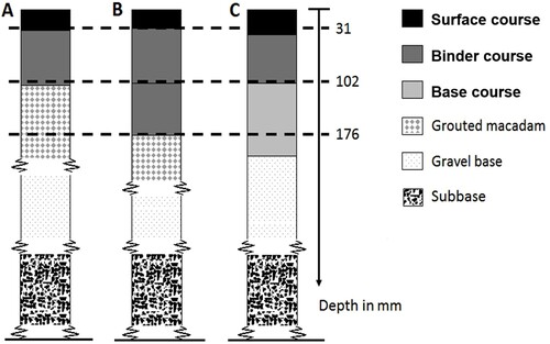
A 7-km bus lane on one of the main streets of Malmö, Sweden, was selected to evaluate rut formation. Since the 1960s, some rehabilitation and maintenance measures have been carried out on-site. The last rehabilitation was conducted in 2014 by milling away approximately 100 mm and replacing it with new asphalt layers, consisting of a binder layer (basecourse) and a wearing course that were designed primarily against rutting. The existing pavement deeper than approximately 100 mm consists of a grouted macadam or a gravel base. Parker and Brown (1992) and Harvey and Popescu (2000) reported that flow rutting in bituminous layers deeper than approximately 100 mm is also negligible. The risk for further deformations in the grouted macadam and the gravel base layers is also minimal due to their location in-depth, age, and many years of traffic loading. Three road sections, denoted A, B and C were chosen in the same direction for this study. The overviews of the sections, each measuring 70 m, are presented in Figure 1. Section B is in front of a signalised intersection. Therefore, although the busses have priority in crossing the intersection, drivers are expected to drive slower as they approach the intersection. Traffic speed is an essential factor in rut formation and as such, requires consideration (Chatti et al. 1996, Wang and Al-Qadi 2010).

Figure 1. A bus lane in the city of Malmö: (a) section A, (b) section B with deceleration area in front of signalised intersection, and (c) section C with curb and physical barrier in the middle.

Transverse profiles were measured at the three road sections to establish the underlying reasons for rutting and to determine rut depths. Falling Weight Deflectometer (FWD) measurements were also performed to check the conditions of the lower layers and to determine if there were significant differences between the sections that might affect the surface (total) rutting. Measured rut depths were used to validate and locally calibrate the estimated rutting from the PEDRO model. Input data for modelling the rutting, such as pavement structures and material properties, were determined from cored specimens. The bus timetables and the region's weather data were utilised to determine the hourly and daily distributions of traffic and temperature, respectively.

Figure 2 shows the pavement structures in sections A, B, and C. The rehabilitation in 2014 consisted of two AC layers, a binder layer of a stone-rich asphalt mixture called Viacobind© 22 mix and a surface layer of an SMA mix called Viacotop© 11 mix. The Viaco-concept is a company-based mix from NCC Road Construction Company containing cellulose fibre (Ulmgren and Lundström 2006). The Viacobind@ 22 mix composition consists of a nominal maximum aggregate size of 22 mm, 4.8% bitumen content by weight (pen 50/70), and 4.8% air void content. The Viacotop@ 11 mix composition consists of a maximum aggregate size of 11 mm, 7% polymer-modified bitumen content by weight, and 3.5% air void content. The exact mix proportions of Viaco-mixes are confidential, and the mix is evaluated by its functional properties. Defining AC properties based only on the mechanical characterisation of the AC is accepted according to the Swedish specification [ATB 2000]. Section B, due to levelling, was paved with several layers of the binder mix after milling of damaged asphalt materials. The AC layer thicknesses of cored specimens from sections A, B, and C showed the surfacing to be 30 , 27 , and 35 mm thick, respectively, and the binder layer thicknesses to be 76 mm, 75 + 74 mm (two lifts), and 66 mm, respectively. The base layer on sections A and B consists of an old, grouted macadam of unknown thickness. Section C has an old base course mix with a thickness of 104 mm.

Figure 2. Pavement structures for sections A, B, and C, where gravel base and sub-base thickness are unknown.

Field measurements

Falling weight deflectometer (FWD)

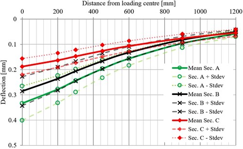
The FWD measurements were conducted with two objectives: first, to understand whether there was a significant difference between the test sections. Secondly, to find out whether the subgrade or lower layers contributed to the total rutting measured on the surface. The FWD were conducted every 10 metres along the three sections following the Swedish specification (TRVMB 2012). Figure 3 shows the average of the deflection measurements with the upper and lower limits of the standard deviations for the measured points from the loading centre. The deflection data shows some differences between the sections, where sections A and B have larger deflections than section C at the loading centre. This should be a result of the differences in the thickness of the pavement structures and the presence of an old base course in section C, as shown in Figure 2. The average deflections in section A are slightly more considerable than in section B, which should be the effect of thicker asphalt layers in section B. Deflection at the loading centre is affected by the pavement strength, including the influence of the stiffness of lower layers. Deflections farthest from the loading centre (> 900 mm) are mainly affected by the stiffness of the lower layers. The low deflections farthest from the loading centre, as shown in Figure 3, indicate a high strength of lower layers. Thus, the contribution of the lower layers to surface rutting is negligible. Consequently, the pavement surface (total) rutting is mainly governed by asphalt mixture properties and the AC layer thicknesses under traffic loading.

Figure 3. Average deflection data ± the measurements’ standard deviation at points from the sections’ loading centre.

Transverse profile measurements

A low-speed laser profilometer called Primal, which has an accuracy of 0.1 mm, was used to measure the transverse profiles of each section (Carlsson 2015). For sections, A and C, measurements were performed every 10 metres, whereas for section B, as it is closer to the traffic signal, measurements were conducted every 5 metres. This allows evaluating the influence of deceleration in speed on rut formation.

The rut depth in the left and right wheel tracks has been calculated from the measured transverse profiles. According to the thread principle, the rut depth calculation is defined as the maximum elevation difference between the transverse profile and a virtual wireline between the profile's endpoints. (Gramling et al. 1991, Carlsson 2015). The average profiles are illustrated in Figure 4 for measurements performed in December 2017. For an accurate estimation of the transverse profile and rut depth development over time, the difference between the original profile before trafficking and subsequent measurements can be calculated rather than using a reference wireline. In this study, the wire method was used as there was no measurements of the original profile. The wire method provides the actual rut depth at a particular time.

Figure 4. Average measured transverse profiles on sections A (a) and C (c) at 35 km/h, and profiles of section B (b) as a function of distance to the stop line with different speeds.

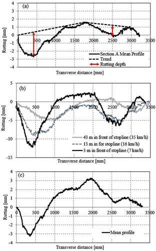
Rutting is usually larger in the left wheel path on normal roads due to differences in vehicle axle width (McGarvey 2016). However, in these sections, only one type of bus is permitted, and differences in rut depth between left and right wheel paths were therefore not expected. The differences in the rut depths are probably caused by horizontal material movement from traffic loading (busses to the opposite direction) at the adjacent lane to the right of the sections. Figure 1 shows the city's narrow lanes, which results in less rut depth (due to upheaval) in the right wheel path of the bus lanes of the sections. Traffic at the adjacent lane on the left side of the sections is primarily cars that have almost no influence on rut formation. The maximum rut depth in the wheel path is affected by the entire rutting zone (ca ± 1.25 metres from tyre loading centre) (Monismith et al. 1994, Blab and Litzka 1995, Siddharthan et al. 2017). The traffic in the adjacent lane might have contributed to reducing the rut depth in the right wheel path. The shape of the profiles with depressions at the wheel track and upheavals in-between the wheel tracks indicate flow rutting in the AC layers. Accordingly, rutting in the left wheel track was used to evaluate the road sections and calibrate the model.

Section B, Figure 4 (b), shows an increase in rut depth closer to the stop line. This resulted from reduced speed from 34 to 7 km/h and due to the effect of the braking action of buses (Wang and Al-Qadi 2010). In addition, the traffic signals may decrease the standard deviation of the lateral wander of busses, which increases rutting. Further investigations would be valuable. The maximum rut depth at a speed of 35 km/h is at Section B (5 mm), and the minimum is at Section A (2.5 mm). The rut depth at Section C (3.2 mm) is in-between. However, slight differences may be related to the thickness and properties of the AC layers of the sections, as illustrated in Figure 2. Consequently, based on falling weight deflection measurements and surface profiles with upheavals, the differences in the surface rut depth of the structures should thus be mainly related to the upper asphalt layers of the pavement structures.

Estimation of rutting profiles

The viscoelastic constitutive relationship reported by Björklund (Björklund 1984) was adopted in the PEDRO model (Oscarsson 2011, Said et al. 2011, Said and Ahmed 2017). The uni-layer PEDRO model calculates permanent deformation in each pavement AC layer and reports the deformation based on the sum of permanent vertical strain in the layers. The model considers crucial variables that affect rutting, such as measured or estimated traffic, climate inputs, and the impact of asphalt mixture aging. The rut prediction was made using the PEDRO v1.10 programme (PEDRO 2019). Required inputs are AC layers properties and thicknesses, vehicle speed, axle load configuration, number of load repetitions, the standard deviation of lateral wander, dimensions of the tyre, and monthly and hourly pavement temperature distribution. The AC layers’ dynamic viscosities of mixes were calculated from shear test data on field-cored samples (Said et al. 2013b, 2021). PEDRO reports surface profile and maximum rut depth since it calculates permanent vertical strains over ± 1.25 metres from the loading centre.

Material characterisation using the shear box

Three AC specimens were drilled from each section, in-between the wheel tracks (less-trafficked area), to determine the viscosities of the mixes. Samples from the recently paved layers in 2014 and the old base course layers were tested in the laboratory. The grouted macadam and old bituminous layers located deeper than 100 mm from the pavement's surface should make only a minor contribution to the surface rutting (Parker and Brown 1992, Harvey and Popescu 2000, Ullidtz et al. 2008). Nevertheless, specimens from old base course layers were also tested using the shear box test. Samples from the grouted macadam could not be tested using the shear test. The master curves of the dynamic shear modulus and phase angle of the AC mixtures from the sections were determined using the frequency sweep shear test at different temperatures (Said et al. 2013b). The shear tests were conducted at frequencies of 0.05, 0.1, 0.5, 1, 2, 4, 8, and 16 Hz and temperatures of −5, 10, 30, and 50°C. The master curves were constructed using a time-temperature superposition principle, and Arrhenius’ equations, Equations 1(1) $Log\left(a_T\right)=R\left({\displaystyle \frac{1}{T+273}-{\displaystyle \frac{1}{T_{ref}+273}}}\right)$(1) and 2(2) $a_T={\displaystyle \frac{f_r}{f_T}}$(2) , were employed to obtain the shift factor (a_T) and reduced frequency at different temperatures. The sigmoidal model, Equation 3(3) $\left|G^{\ast }\right|=\delta +{\displaystyle \frac{\text{β}}{1+e^{-\lambda \left(f_r-\gamma \right)}}}$(3) , was used to fit shear modulus data, and the compound sigmoidal and unimodal model, Equation 4(4) $\mathrm{\varnothing }=d\cdot \left(1-{\displaystyle \frac{e^{\left({\displaystyle \frac{f_r-a}{g}}\right)}}{1+e^{\left({\displaystyle \frac{f_r-a}{g}}\right)}}}\right)+c\cdot \left({\displaystyle \frac{1}{1+{\left({\displaystyle \frac{f_r-a}{b}}\right)}^2}}\right)$(4) , was used to fit the phase angle data. The master curves of the dynamic shear moduli and phase angles for the mixes calculated at a reference temperature (T_ref) of 10°C are shown in Figures 5–7. (1) $Log\left(a_T\right)=R\left({\displaystyle \frac{1}{T+273}-{\displaystyle \frac{1}{T_{ref}+273}}}\right)$(1) (2) $a_T={\displaystyle \frac{f_r}{f_T}}$(2) (3) $\left|G^{\ast }\right|=\delta +{\displaystyle \frac{\text{β}}{1+e^{-\lambda \left(f_r-\gamma \right)}}}$(3) (4) $\mathrm{\varnothing }=d\cdot \left(1-{\displaystyle \frac{e^{\left({\displaystyle \frac{f_r-a}{g}}\right)}}{1+e^{\left({\displaystyle \frac{f_r-a}{g}}\right)}}}\right)+c\cdot \left({\displaystyle \frac{1}{1+{\left({\displaystyle \frac{f_r-a}{b}}\right)}^2}}\right)$(4) where a_T is the shift factor, T is test temperature in ^oC, T_ref is the reference temperature 10 ^oC, R is the Arrhenius constant (approximately 10,920 or preferably estimated during the curve fitting to master curves), f_r is reduced frequency, f_T is the frequency at temperature T, |G*| is dynamic shear modulus, ϕ is phase angle and δ, β, λ, γ, a, b, c, d, g are master curves fitting parameters. The shear modulus and phase angle master curves in Figure 5 represent the three sectionś surface mix. Figure 5 also shows an example of the master curves fitting by testing three specimens.

Figure 5. Phase angle and shear modulus master curves at 10 ^oC for surface layer mix, Viacotop 11.

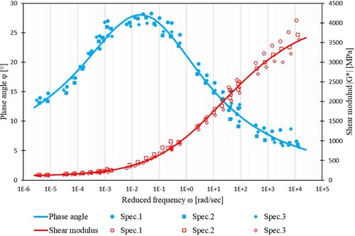
Figure 6. Phase angle and shear modulus master curves at 10 ^oC for binder layers mixtures of the sections A, B, and C, Vicobind 22.

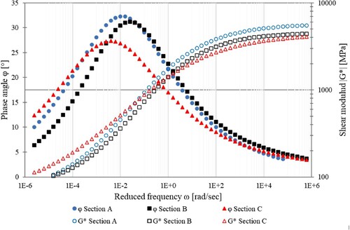
Figure 7. Phase angle and shear modulus master curves at 10 ^oC for base course (old base course) of the section C.

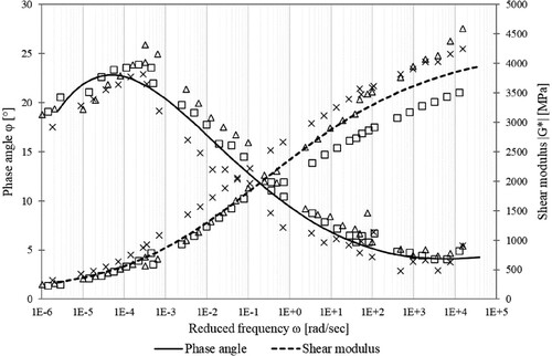
The curve fitted master curves of shear moduli and phase angles of the binder layers of the sections and the old base course of section C are presented in Figure 6 and Figure 7, respectively. Low phase angle values and offset of phase angle to the left side indicate the material’s high resistance to permanent deformation. The binder layer mix of section C shows a better resistance to permanent deformation than the binder mixes of sections A and B. The old-aged base course mix shown in Figure 7 indicates a significantly better resistance to permanent deformation than binder and surface mixtures. Rutting resistance of asphalt mixtures can be practically characterised by determining dynamic viscosity. The viscosity of AC is the main parameter to characterise an asphalt mix in the PEDRO model. The dynamic viscosity of a mix at maximum phase angle is determined according to Equation 5(5) $\left|{\eta }^{\ast }\right|={\displaystyle \frac{\left|G^{\ast }\right|}{\omega }}$(5) , where the ratio of the lost to the stored deformation energy is maximum (tan ϕ = G"/G´) at the corresponding temperature. (5) $\left|{\eta }^{\ast }\right|={\displaystyle \frac{\left|G^{\ast }\right|}{\omega }}$(5) where η* is complex viscosity at maximum phase angle in MPa s, G* is complex shear modulus in MPa, and ω is the angular frequency in rad/sec.

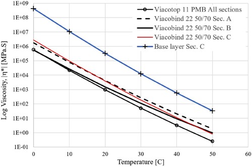
At intermediate temperatures and frequencies (approximately zero reduced frequency), the old base layer (Figure 7) showed the highest shear modulus, while the surface layer (Figure 5) showed the lowest shear modulus. The binder layers (Figure 6) are somewhere in-between. The maximum phase angle of the old base layer is noticeably smaller and occurs at a significantly lower frequency than the other mixes. This indicates the old base mix’s high rutting resistance compared to the recently laid mixes, which may be due to aging. The mixture viscosity demonstrates the combined influence of the shear modulus and the phase angle. Figure 8 shows the dynamic viscosities of the mixes determined at different temperatures using Equation 5(5) $\left|{\eta }^{\ast }\right|={\displaystyle \frac{\left|G^{\ast }\right|}{\omega }}$(5) . The deformation resistance of mixes at elevated temperatures when compared using their viscosities is lowest for the surface layer and highest for the old base layer.

Figure 8. The viscosity of surfacing (Viacotop 11), binder layers (Viacobind 22), and base layer as a function of temperature.

Traffic loading

The traffic volume of the buses was calculated from the bus timetables for the different seasons for three years (2014–2016), with minor differences between seasons. The mean annual average daily traffic (AADT) was calculated to be 129 vehicles per day based on the fixed bus schedule.

The annual traffic growth rate was assumed to be 0%, and no significant changes were reported during the study period (i.e. 2014–2016). The buses are 23.82 m long and have a service weight of 245 kN and a total gross weight of 365 kN. Technical data of the buses that are essential for rut prediction are shown in Table 2. Figure 9 shows the frequency and hourly distributions of buses. The hourly distribution is used to isochrone traffic loading with temperature. The frequency distribution data, expressed as a function of time, was fitted to a mathematical function using Equations 6a and 6b. (Said et al. 2020, 2021). (6a) $\mathrm{\varnothing }={\displaystyle \frac{2\pi \ast \left(t+{\text{β}}_3\right)}{24}}$(6a) (6b) $\begin{array}{rl}& Y={\text{β}}_0+{\text{β}}_1\ast \\ & \left[{\displaystyle \frac{{\text{β}}_2}{1+{\left(\tan \mathrm{\varnothing }\right)}^2}+sign(\mathrm{s}\mathrm{i}\mathrm{n}\mathrm{\varnothing }\ast \sqrt{{\left({\displaystyle \frac{{\text{β}}_2}{1+{\left(tan\mathrm{\varnothing }\right)}^2}}\right)}^2-{\displaystyle \frac{{\text{β}}_2^2-{\left(tan\mathrm{\varnothing }\right)}^2}{{\left(\tan \mathrm{\varnothing }\right)}^2+1}}}}\right]\end{array}$(6b) Where ϕ is the time parameter, t is time in hours, β₀ (0.036), β₁ (0.018), β₂ (0.603) and β₃ (13.50) are constants in the fitting functions, and Y is frequency distribution data.

Figure 9. Hourly traffic distribution of busses 2014–2016.

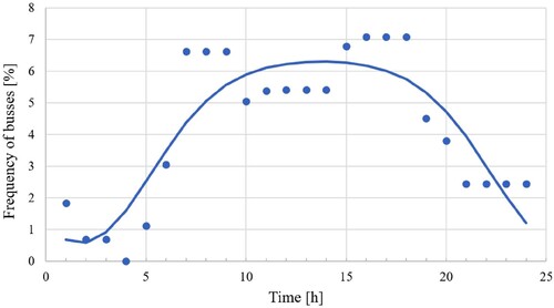
Table 2. Tire configuration on each axle and bus technical data.

Axle no.	Configuration	Tire dimension	Permissible axle load (kg)	Track width c-c (mm)
1	Single (steering axle)	275/70R22.5 (Hankook e-cube DL10)	7245	2140
2	Dual (driven axle)		11500	1900
3	Dual		10000	1900
4	Single		7245	2140

The bus weight was calculated to be, on average, assuming a 50% passenger occupancy plus the technical service weight. The weight of the passengers is distributed as a percentage per axle based on the technically permissible weight. The single axles No 1 (steering axle) and No 4 were calculated from an axle weight of 61 kN each. The dual configurations axle No 2 and No 3 were estimated to be 97 and 84 kN, respectively.

The tyre-pavement contact pressure depends mainly on tyre type and dimensions, wheel load, and inflation pressure (De Beer et al. 2005, Al-Qadi et al. 2012). The PEDRO software assumes a uniformly distributed tyre contact pressure within a circular area. The contact pressure for the bus tyre Hankook e-cube DL10, 275/70R22.5, was calculated for axle load and tyre inflation pressure (0.9 MPa) using Equation 7(6b) $\begin{array}{rl}& Y={\text{β}}_0+{\text{β}}_1\ast \\ & \left[{\displaystyle \frac{{\text{β}}_2}{1+{\left(\tan \mathrm{\varnothing }\right)}^2}+sign(\mathrm{s}\mathrm{i}\mathrm{n}\mathrm{\varnothing }\ast \sqrt{{\left({\displaystyle \frac{{\text{β}}_2}{1+{\left(tan\mathrm{\varnothing }\right)}^2}}\right)}^2-{\displaystyle \frac{{\text{β}}_2^2-{\left(tan\mathrm{\varnothing }\right)}^2}{{\left(\tan \mathrm{\varnothing }\right)}^2+1}}}}\right]\end{array}$(6b) , which was established through tyre footprint measurements that were conducted using different wheel loads and tyre inflation pressures (Said et al. 2020). 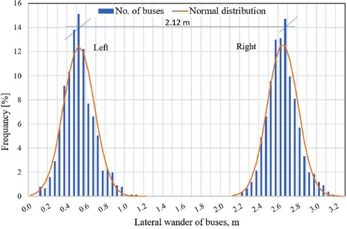(7) $\sigma =80.09+0.28\cdot p_i+9.72\cdot P$(7) Where σ is contact pressure in kPa, p_i is tyre pressure in kPa, and P is tyre load in kN. The measured standard deviation of the lateral wander illustrated in Figure 10, and the speed of bus traffic were 0.16 m and 34.5 km/h, respectively, measured using coaxial cable sensors (McGarvey 2016, 2017). The measured lateral wander is much smaller than the values reported in other studies for highways and freeways, where the standard deviation is often in the range of 0.25-0.30 m (McGarvey 2016). This is due to limited space in urban streets but also the relatively low allowable speeds.

Figure 10. Normal distribution of lateral wander of traffic.

Pavement temperature

Temperature data from 2012 to 2016 from three weather stations located on the outskirts of the city of Malmö were used to estimate the average monthly and hourly temperature distributions at the mid-depth of each AC layer of the pavement. A climate model by Hermansson and Elsander (2003) was used to calculate the temperature distribution. Figure 11 illustrates examples of the climate data used as input to the PEDRO model. The traffic and pavement temperature distribution peaks occur at almost the same time of the day as can be seen in Figures 10 and 12. This is essential in rutting prediction.

Figure 11. Monthly and hourly temperature distributions at mid of the surface layer, 0.017 m, and mid of the binder layer, 0.068 m, below the road surface.

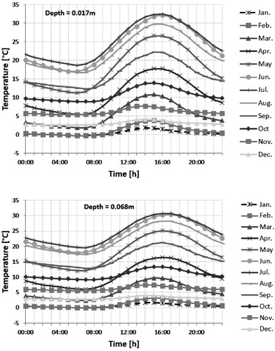
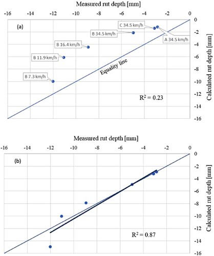
Figure 12. Relationship between measured and calculated rut depth with the coefficient of determination (R2), (a) using the default calibration factor and, (b) after the local calibration.

Analysis and local calibration

Figure 12(a) shows the calculated and measured rut depths for the studied sections. The rut depths were calculated using the default calibration factor of the PEDRO model (0.02). Figure 12(a) also illustrates considerable differences between the measured and calculated rut depths. The coefficient of determination R² was 0.23, indicating a poor agreement between the measured and predicted values. Local calibration was, therefore, crucial for better prognoses of rut development in the field (Salama et al. 2007, Habbouche et al. 2019). Distinct differences between the sections were the total thickness of the pavement's AC layers and the variation in bus speed in section B. The range of variation in the values of other parameters, such as viscosity and traffic loading, was limited in this study. Equation 8(7) $\sigma =80.09+0.28\cdot p_i+9.72\cdot P$(7) was established to determine the sections’ local calibration factor (CF_L). (8) $C{F}_L=0.031\ast V-8.7\cdot {10}^{-4}\ast h+1.428$(8) where h is the total thickness of bituminous layers in mm, and V is traffic speed in km/h. Figure 12(b) shows the correlation between the measured and calculated rutting after local calibration with a coefficient of determination R² equal to 0.87. Rutting prediction after local calibration, which is helpful for maintenance planning, is determined by multiplying the calculated rutting using a factor that is the product of the default calibration factor (CF) and the local calibration factor (CF_L) as presented in Figure 12(b). The local calibration was established based on rutting measurements from three and half years of traffic, a short period, with relatively small deformations. The maximum deviation between the predicted and measured values at larger rutting depths, e.g. at 11.1 mm, was about 9.2%. The CF_L is mainly applied for maintenance planning of existing roads in anticipation of more reliable general CF, which can also be used in the pavement design of new roads. The number of variables and the range of variation in the values of parameters used in the calibration processes was also limited in this study. A general calibration procedure with repeated measurements over a longer time would be valuable.

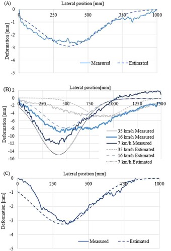
The calculated rutting profiles were calibrated using measurements that were taken from the left wheel path. Figure 13 shows the mean profiles of sections A and C at a free-rolling bus speed of 35 km/h compared to predicted profiles after local calibration. The profiles in section B are at different speeds, depending on the distance from the stop line. As can be seen in Figure 13, the predicted rutting profiles with local calibration agree well with measured section B profiles, except for the profile at a speed of 7.3 km/h where nearly 20% overestimation of rut depth is observed. Examples of profiles from section B with the effect of traffic speed are illustrated in Figure 13.

Figure 13. Measured and predicted transverse profiles for road sections A and C at a speed of 35 km/h and section B at speeds of 7, 16, and 35 km/h.

The prediction of rut development over time was performed for each layer from the construction date, 2014, and forward for 20 years, as shown in Figure 14. Due to post-compaction, the first phase of the rutting occurs mainly in the surface layer (Björklund 1984, ARA 2004) and gradually lasts over 2 −3 years after construction (Said et al. 2011, Said and Ahmed 2017). Shear deformation dominates rut development in the secondary phase. As seen in Figure 14, the rut development due to shear distortion primarily occurs in the binder layers, which were located at a depth of maximum shear stresses. This indicates the importance of binder layer mixes to withstand rut formation. The old base layer shows minor rutting as it is located at a greater depth from the surface within the structure and has high viscosity (Figure 8) related to its age. Unfortunately, only one measurement of transverse profiles has been performed, as shown in Figure 14. Future field measurements will be valuable to validate the rut depth development over time.

Figure 14. Measured and predicted the development of rutting for road sections A (a), B (b), and C (c).

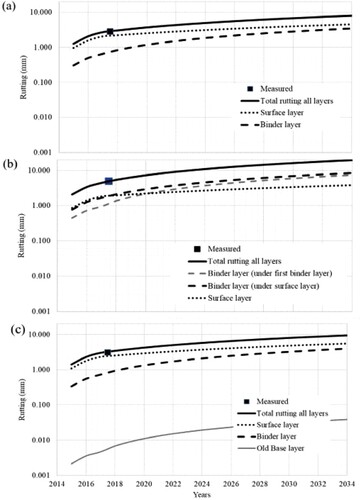
The underlying binder layer in section B shows minor deformation than the upper binder layer, see Figure 14b, which supports the theory that the maximum vertical stress occurs about 50–120 mm below the road surface, and the stresses decrease gradually with the depth of the structure (Parker and Brown 1992, Harvey and Popescu 2000, Wang and Al-Qadi 2010, Said et al. 2011, 2017).

It can be stated that PEDRO’s prediction can be a helpful tool for maintenance and rehabilitation strategy as well as to control rutting through a mix design of bituminous pavement layers. For example, from the outcome of this study, it can be recommended to rehabilitate a section depending on the allowed rutting. However, sections in front of signalised intersections should be rehabilitated with higher viscosity mixes to withstand excess deformations due to the influence of braking and lower traffic speed. This could be an essential input in cost–benefit maintenance planning.

Conclusions and recommendation

The PEDRO performance prediction model, which uses viscoelastic theory, was applied in this study to predict rut development and transverse profile, facilitating the implementation of the model for bus lanes. The model was applied to three road sections with different structures on a bus lane in an urban expressway. One of the sections is located close to an intersection where traffic speed is expected to decrease significantly. Traffic loading, the lateral traffic wander of the buses, the tyre-pavement contact pressure, and the bus speed, hourly distribution of buses and temperatures were considered as inputs in PEDRO. Asphalt concrete rheological properties that are required inputs to the model were determined based on the dynamic shear test on cored specimens. The following conclusions and recommendations are derived from the study:

• The PEDRO performance model has the potential to distinguish rutting in each asphalt pavement layer, which is helpful in pavement design and maintenance applications, including a selection of asphalt mixtures for each pavement layer to withstand permanent deformation.

• The PEDRO model distinguishes permanent deformations related to densification (post-compaction) and shear distortion over time. Rut depth development and transverse profile with depression and upheaval per asphalt concrete layer are reported.

• The PEDRO model was successfully calibrated for the road sections with a deviation of less than 10%. It is adequately accurate, practical, and easy to study the influences of the main parameters on rut formation in asphalt concrete materials.

• A general calibration procedure considering field condition uncertainty and including all required variables is recommended to improve the prediction of the PEDRO model further.

• The influence of braking and lower traffic speed at typical braking areas, such as intersections, should be accounted for in rutting prediction models.

• Extending the PEDRO model to a multilayer rutting model should enhance the precision of rut prediction.

Acknowledgment

Malmö City, Lund University, the strategic innovation programme, InfraSweden2030, the Swedish Transportation Administration, the Development Fund of the Swedish Construction Industry (SBUF), and Nynas AB Product Technology are acknowledged for their financial support. NCC Company provided technical field support. Håkan Carlsson (VTI) is recognised for his technical support.

Disclosure statement

No potential conflict of interest was reported by the author(s).

References

- Abdallah, I., and Nazarian, S., 2011. Strategies to improve and preserve flexible pavement at intersections. Publication FHWA/TX 10/0-5566-1, Center for Transportation Infrastructure Systems. The University of Texas, El Paso, Texas.
- Al-Qadi, I.L., Elseifi, M.A., and Yoo, P.J., 2004. Pavement damage Due to different tires and vehicle configurations. Blacksburg: Virginia Tech Transportation Institute.
- Al-Qadi, I.L., and Wang, H., 2012. Impact of wide-base tires on pavements: results from instrumentation measurements and modeling analysis. Transportation Research Record, 2304 (1), 169–176. doi:10.3141/2304-19.
- Ali, B., Sadek, M., and Shahrour, I., 2009. Finite-element model for urban pavement rutting: analysis of pavement rehabilitation methods. Journal of Transportation Engineering, 2009, 235–240.
- ARA, 2004. Guide for the Mechanistic empirical design of new and rehabilitated pavement structure. (Report 1-37A), Washington, D. C: Transportation Research Board of the National Academies.
- ATB, 2000. General technical construction specifications for roads (ATB väg 2000), Swedish Transport Administration, Borlänge, Sweden (In Swedish).
- Björklund, A., 1984. Creep induced behaviour of resurfaced pavements, VTI Report 271A, The Swedish National Road and Transport Research Institute, Linköping, Sweden.
- Blab, R., and Litzka, J., 1995. Measurements of the lateral distribution of heavy vehicles and its effects on the design of road pavements. Vienna, Austria: Institute of Road Construction and Maintenance, University of Technology.
- Carlsson, H., 2015. Profilmätning på sträckor med gummimodifierat bitumen på E4 Uppsala och E6 Mölndal, Uppföljning efter tre års Trafik. VTI Notat 5-2015, The Swedish National Road and Transport Research Institute, Linköping, Sweden., (In Swedish).
- Chatti, K., et al., 1996. Field investigation into effects of vehicle speed and tire pressure on asphalt concrete pavement strains, TRR 1539. https://doi.org/10.1177/0361198196153900109.
- Corté, J-F., et al., 1994. Investigation of rutting of asphalt surface layers: influence of binder and axle loading configuration. Transportation Research Record, 1436, 28–37.
- De Beer, M., et al., 2005. Tyre-pavement contact stress patterns from the test tyres of the Gautrans heavy vehicle simulator (HVS) MK IV+, Proc. of the SATC 2005.
- Di Benedetto, H., Delaporte, B., and Sauzéat, C., 2007. Three-dimensional linear behavior of bituminous materials: experiments and modeling. International Journal of Geomechanics, 7 (2), doi:10.1061/(ASCE)1532-3641(2007)7:2(149).
- El-Basyouny, M.M., Witczak, M.W., and El-Badawy, S., 2005. Verification for the calibrated permanent deformation models for the 2002 design guide. Journal of the Association of Asphalt Pavement Technologists, 74, 601–652.
- Erlingsson, S., Said, S., and McGgarvey, T., 2012. Influence of heavy traffic lateral wander on pavement deterioration. The 4th European pavement Asset Management Conference, Malmö, Sweden.
- Garba, R., 2002. Permanent Deformation Properties of Asphalt Concrete Mixtures. The Department of Road and Railway Engineering, Norwegian University of Science and Technology.
- Gramling, W.L., Hunt, J. E., and Suzuki, G.S., 1991. Rational approach to cross-profile and Rut depth analysis. Transportation Research Record, 1311, 173–179.
- Habbouche, J., Hajj, E.Y., and Sebaaly, P.E., 2019. Structural coefficient for high polymer modified asphalt mixes. Contract No. BE321, Final Report, Department of Civil and Environmental Engineering, University of Nevada, Reno.
- Hajj, E.Y., Tannoury, G., and Sebaaly, P.E., 2011. Evaluation of Rut resistant asphalt mixtures for intersection. Road Materials and Pavement Design, 12, 263–292. doi:10.3166/RMPD.12.263-292.
- Harvey, J., and Popescu, L., 2000. Rutting of caltrans asphalt concrete and asphalt-rubber hot mix under different wheels, tires and temperature-accelerated pavement testing evaluation. Berkeley: Pavement Research Center, Institute of Transportation Studies, University of California.
- Hermansson, Å., and Elsander, J., 2003. Prediction of pavement fatigue life with simulated temperature profile from hourly surface temperatures. Road Materials and Pavement Design, 4 (3), 293–308. doi:10.1080/14680629.2003.9689950.
- Hopman, P.C, 1996. The visco-elastic multilayer program VEROAD. HERON, 41 (1), 71–91. Univ. of Delft, The Netherland.
- Hua, J., and White, T., 2002. A study of nonlinear tire contact pressure effects on HMA rutting. International Journal of Geomechanics, 2 (3), 353–376. doi:10.1061/(ASCE)1532-3641(2002)2.
- Jelagin, D., et al., 2018. Asphalt layer rutting performance prediction tools. VTI Report 968A, VTI, Linköping.
- Kaloush, K.E., Witczak, M.W., and Sullivan, B. W., 2003. Simple performance test for permanent deformation evaluation of asphalt mixtures. 6th International RILEM Symposium on Performance Testing and Evaluation of Bituminous Materials, 2003, 498–505. https://doi.org/10.1617/2912143772.062.
- Kandhal, P.S., Mallick, R.B., and Brown, E. R., 1998. Hot mix asphalt for intersections in hot climates. NCAT Report 98-06, Auburn.
- Kenis, W., and Wang, W., 1997. Calibrating mechanistic flexible pavement rutting models from full scale accelerated tests. 8th Int. conference on asphalt pavements, Seattle.
- Li, L., et al., 2013. Integrated experimental and numerical study on permanent deformation of asphalt pavement at intersections. July, 907–913. https://doi.org/10.1061/(ASCE)MT.1943-5533.0000745.
- McGarvey, T., 2016. Vehicle lateral position depending on road type and lane width vehicle position surveys carried out on the swedish road network. VTI Report 892A, The Swedish National Road and Transport Research Institute, Linköping, Sweden.
- McGarvey, T., 2017. Barrier separated road type design accelerated degradation. VTI Report 925A, The Swedish National Road and Transport Research Institute, Linköping, Sweden.
- Monismith, C. L, et al., 1994. SHRP report A-415: permanent deformation response of asphalt aggregate mixes. asphalt research program. Berkeley: Institute of Transportation Studies, University of California. Transportation Research, Washington, D.C.
- Nilsson, R., 2001. Viscoelastic pavement analysis using VEROAD. Thesis (PhD), KTH Royal Institute of Technology, Stockholm, 2001.
- Oscarsson, E., 2011. Mechanistic-empirical modeling of permanent deformation in asphalt concrete layers. Thesis (PhD), Department of Technology and Society, Lund University, Lund, 2011. ISBN 978-91-7473-083-8.
- Park, D.W, 2008. Prediction of pavement fatigue and rutting life using different tire types. KSCE Journal of Civil Engineering, 12 (5), 297–303. doi:10.1007/s12205-008-0297-4.
- Parker, F., and Brown, E.R., 1992. Effects of aggregate properties on flexible pavement rutting in Alabama. ASTM STP, 1147, 68–89.
- PEDRO online, 2021. [software]. https://pedro.vti.se . Accessed Mars, 2022.
- PEDRO v1.10, 2019. [software]. https://www.vti.se/en/research-areas/pavement-design-models-for-roads /. Accessed Mars, 2022.
- Rana, M.M., and Hossain, K., 2021. Impact of autonomous truck implementation: rutting and highway safety perspectives. Road Materials and Pavement Design, doi:10.1080/14680629.2021.1963815.
- Said, S.F., et al., 2011. Prediction of flow rutting in asphalt concrete layers. International Journal of Pavement Engineering, 12 (6), 519–532. doi:10.1080/10298436.2011.559549.
- Said, S.F., 2015. Tyre-pavement interaction on flexible pavement rutting. The XXVth World Road Congress (PIARC), Seoul. South Korea.
- Said, S.F, et al., 2020. Prediction of rutting in asphalt concrete pavements – the PEDRO model, VTI rapport 1016A, The Swedish National Road and Transport Research Institute, Linköping, Sweden.
- Said, S.F., and Ahmed, A. W., 2017. Prediction of heavy vehicle impact on rut development using PEDRO Model. Proceeding of the 10th Int. Conference on the Bearing Capacity of Roads, Railways and Airfields, Athena,1359–1366.
- Said, SF., Carlsson, H., and Ahmed, A.W., 2021. Long-term pavement performance road test E6 with polymer modified bitumen – Uddevalla, VTI rapport 1096, The Swedish National Road and Transport Research Institute, Linköping, Sweden.
- Said, S.F., and Hakim, H., 2012. Influence of traffic variables on rut formation in asphalt concrete layers, Heavy Vehicle Transport and Technology Conference, Stockholm, Sweden.
- Said, S.F., and Hakim, H., 2013a. Effects of transversal distribution of heavy vehicles on Rut formation in Bituminous Layers. Proceedings of the 9th Int. Conf. BCRRA, Trondheim, Norway, 29–35.
- Said, S.F., Hakim, H., and Eriksson, O., 2013b. Rheological characterization of asphalt concrete using a shear Box. Journal of Testing and Evaluation, 41 (4), doi:10.1520/JTE20120177.
- Salama, H.K., Haider, S.W., and Chatti, K., 2007. Evaluation of new mechanistic-empirical pavement design guide rutting models for multiple-axle loads, Transportation Research Record, TRR No. 2005, pp. 112-123.
- Siddharthan, R.V., et al., 2017. Investigation of impact of wheel wander on pavement performance. Road Materials and Pavement Design, 18 (2), 390–407. doi:10.1080/14680629.2016.1162730.
- Soares, R.F., et al., 2008. A computational model for predicting the effect of tire configuration on asphaltic pavement life. Road Materials and Pavement Design, 9 (2), doi:10.3166/rmpd.9.271-289.
- Sousa, J., Craus, J., and Monismith, C., 1991. Summary report on permanent deformation in asphalt concrete. SHRP-A/IR-91-104, Project A-003A, University of California, Berkeley.
- Timm, D.H., and Priest, A.L, 2005. Wheel wander at the NCAT Test Track, NCAT Report 05-02, National Center for Asphalt Technology (NCAT), Auburn University.
- TRVMB, 2012. Deflektionsmätning Vid Provbelastning Med Fallviktsapparat. Swedish Transport Administration, Borlänge, Sweden (In Swedish).
- Ullidtz, P., et al., 2008. Calibration of mechanistic-empirical models for flexible pavements using the WesTrack experiment. Journal of the Association of Asphalt Paving Technologists (AAPT), 77, 591–630.
- Ulmgren, N., and Lundström, R., 2006. The SMA-principle applied to wearing, binder and base course layers – the VIACO-concept, 10th International Conference on Asphalt Pavements, ISAP Qubéc 2006.
- Wang, H., 2011. Analysis of tire-pavement interaction and pavement responses using a decoupled modeling approach. University of Illinois at Urbana-Champaign, Urbana, Illinois.
- Wang, H., and Al-Qadi, I. L., 2010. Evaluation of surface-related pavement damage Due to tire braking. Road Materials and Pavement Design, 11 (1), 101–121. doi:10.1080/14680629.2010.9690262.
- Wiman, L.G., et al., 2009. Prov med olika överbyggnadstyper. E6 Fastarp-Heberg. VTI rapport 632, The Swedish National Road and Transport Research Institute, (In Swedish).