Automated Dielectric Thermoscopy Characterization of Water-Contaminated Grease

Abstract

Machine maintenance is important for improving machine uptime and reliability, and for reducing costs. Grease is used in most rolling element bearings, and one common failure criterion is water contamination, so developing a sensor that can detect water content automatically without human input could be a useful endeavor. The temperature dependence on the dielectric properties of water-contaminated grease is investigated in this article with computer logged instrumentation. This method has been termed dielectric thermoscopy (DT). Several off-the-shelf (two lithium, one lithium complex, and two calcium sulfonate complex) and one unadditivized lithium grease are tested with varying amounts of water contamination from 0% to approximately 5%. Another grease is tested with small increments of added water from 0% to 0.97% to test the resolution of the measurement. The purpose is to use the capacitance temperature slope (termed dielectric thermoscopy) to show correlations to the water content of the grease sample and investigate whether any grease types will pose problems in the measurement. A small, custom-made fringe field capacitance sensor with an integrated temperature sensor has been used for this characterization, and data are logged automatically with laboratory equipment and a personal computer (PC). A useable and positive correlation to water content and the DT measurement of roughly 0.5 pF per 10 °C and percentage of water was found, although it was found that some greases have different behavior than others.

Keywords:

• Greases
• water contamination
• oil condition monitoring

Introduction

Machine maintenance is important for operating machinery sustainably and as cheaply as possible. Grease-lubricated bearings are ubiquitous throughout industry and everyday life. They exist in everything from rollerskate bearings to multi-meter-diameter wind turbine bearings.

Large machinery can have maintenance costs that cover 15–60% of the total cost of operation (1). Thus, the performance and cost-effectiveness of the machine can be improved by appropriate maintenance methods. Since practically all moving machines have rolling element bearings, and most rolling element bearings use grease as a lubricant, knowing when grease fails is a good start to improving reliability. Methods to predict this could include predictive algorithms based on heuristics (2) that use operating conditions to approximate the remaining useful life from previously measured data, or methods that take direct measurements. The latter require sensors for measuring the component of the machine for which prediction of failure is desired. In the case of this article, that is lubricating grease.

Some existing technologies include vibration or acoustic emission measurements to detect damage or particle contamination (3); however, this will only detect failure after some damage has already occurred. Since water is related to decreasing lubricant performance but is not guaranteed to cause instant failure (4,5), detecting water and allowing the machine to discontinue operation could prevent costly damage to components.

For a more complete background, a previous thesis discusses reasons why and how performing grease lubrication maintenance at intervals determined by condition monitoring tools can improve machine reliability, how grease degrades, and how grease composition presents a difficult problem for sensor development (6).

Dielectric thermoscopy (DT) is a measurement to estimate the water content of water-contaminated lubricating grease. It was discovered that the capacitance temperature slope (dC/dT) provides a better correlation to water content than a traditional capacitance measurement. Essentially, the capacitance is measured over a temperature change and the slope is calculated. It was observed that the slope is linear within the temperature range used.

The objective of this article is to further characterize the use of the DT measurement for measuring water content of grease introduced in (7) with automated measurements and the next iteration of sensor development. In the previous study, grease sensor coverage was already considered and is therefore not considered in this article. This early research was also a manual experiment, requiring a person to log data and operate the measurement equipment manually. It also only considered one type of grease. In this new article, we introduce computer equipment to log the same data as before at consistent time intervals and with a controlled heating system to show trends over time and allow for a more complete analysis of sensor performance. This shows that it should be possible to use this method in an embedded device to log data in situ in a machine. The next iteration of sensor development entails custom-made sensor boards, miniaturized and optimized according to previous experiments. The temperature change also includes a heating and cooling cycle, instead of merely increasing the temperature. The cooling cycle is when the sensor passively cools down toward the ambient temperature of the room. This enables a better analysis of the measurement in other conditions. Additionally, several types of lithium and calcium sulfonate complex greases are measured in order to ascertain whether some grease chemistries will cause problems, which broadens the scope of the technique. The second section of this article reviews the concept of dielectric thermoscopy and introduces the hardware and measurements used in this investigation. The third section specifies the different greases used in this investigation and the procedure for preparing the grease samples, and presents results from the experiments performed. The article ends with a section discussing the scope of this report and some concluding remarks.

Dielectric thermoscopy

The configuration of the DT sensor is shown in next, and the heating system for the sensor is then described. The data acquisition and analysis follow, and then the measurement procedure used to verify the performance of the sensor in this article. In this experiment, a custom-made sensor is temperature controlled with a heating system to represent the temperature change in an application. The capacitance and temperature are logged automatically for calculation on a computer.

Sensor design

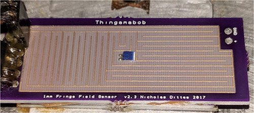
The fringe field sensor board used in this experiment is shown in Fig. 1. It is a custom-made printed circuit board (PCB). The temperature sensor seen in the center of the sensor is a PT100 thin-film platinum resistance temperature detector (RTD). This model RTD was chosen for its very small footprint, extremely small thermal mass, non-electrically conductive case, chemical-resistant case, and ease of installation. This was epoxied to the surface on the center of the fringe field sensor.

Figure 1. The fringe field sensor. The traces are 0.2 mm and the separation distance is 1 mm. The traces are coated with an industry standard ENIG (electroless nickel immersion gold) coating to help ensure the surface properties remain constant. The sensor is 20 × 50 mm. The PT100 temperature sensor is on the center of the sensor board.

The theoretical performance of the sensor is given next. A similar derivation is given in (7); however, the theory has since then been further modified in this article to accommodate estimating the difference due to a thin coating with a different dielectric constant in between the traces and on top. This could be useful if it is found that coatings of a different hydrophobicity help improve the performance or behavior of the sensor with different greases. The coating can be calculated as zero if there is no coating, as is the case for this article.

The calculation for an approximation for this configuration of an interdigitated fringe field capacitor, where the capacitance of one “line” is (8) [1] $${\mathit{C}}_{\mathit{line}}={\mathit{\epsilon }}_0\left({\mathit{\epsilon }}_{\mathit{pcb}}+{\mathit{\epsilon }}_{\mathit{g}}{\mathit{A}}_{\mathit{g}}+{\mathit{\epsilon }}_{\mathit{c}}{\mathit{A}}_{\mathit{c}}\right)\frac{\mathit{K}\left({\mathit{k}}_1\right)}{\mathit{K}\left({\mathit{k}}_2\right)}+2{\mathit{\epsilon }}_0{\mathit{\epsilon }}_{\mathit{c}}\frac{\mathit{t}}{\mathit{s}}$$[1] where ε_o is the electric permittivity of free space ($8.85\mathrm{ }\times \mathrm{ }{10}^{-12}\mathrm{F}/\mathrm{m}$ ); ε_pcb, ε_g, and ε_c are the relative dielectric constants of the PCB material, grease sample on the sensor, and coating respectively; and A₁ and A₂ represent the estimated area of the cross section of the fringe field above the surface of the sensor traces (the grease and coating, respectively). The variable s represents the distance between the traces (edge to edge), and t is the thickness of the digits (the copper traces on the PCB).

The areas A_g and A_c can be calculated as [2] $${\mathit{A}}_{\mathit{g}}=\frac{{\mathit{r}}^2}{2}\mathrm{ }\left(\mathit{\theta }-\text{sin}\left(\mathit{\theta }\right)\right),\mathrm{ }{\mathrm{ }\mathit{A}}_{\mathit{c}}=\mathit{\pi }{\frac{\mathit{r}}{2}}^2-{\mathit{A}}_{\mathit{g}},$$[2] $$\mathit{\theta }=\mathrm{ }\mathit{\pi }-2{(\text{tan}}^{-1}\left(\frac{{\mathit{t}}_{\mathit{c}}}{\mathit{r}}\right)),\mathrm{ }\mathit{r}=\frac{(\mathit{t}+\mathit{s})}{2},$$ where the areas of a thin film coating (solder mask) and grease on the surface are assumed to fit within a semicircular profile. The coating thickness is $t_c$ $\mathrm{t}\_\mathrm{c}$ $.$ The variables k₁ and k₂ can be calculated as [3] $${\mathrm{ }\mathit{k}}_1=\sqrt{1-{\left(\frac{\mathit{w}}{2\left(\mathit{w}+\mathit{s}\right)}\right)}^2},{\mathrm{ }\mathit{k}}_2=\frac{\mathit{w}}{2\left(\mathit{w}+\mathit{s}\right)},$$[3] where w is the width of the digits, and s again is the distance between the traces (edge to edge). The function K in Eq. [1][1] $${\mathit{C}}_{\mathit{line}}={\mathit{\epsilon }}_0\left({\mathit{\epsilon }}_{\mathit{pcb}}+{\mathit{\epsilon }}_{\mathit{g}}{\mathit{A}}_{\mathit{g}}+{\mathit{\epsilon }}_{\mathit{c}}{\mathit{A}}_{\mathit{c}}\right)\frac{\mathit{K}\left({\mathit{k}}_1\right)}{\mathit{K}\left({\mathit{k}}_2\right)}+2{\mathit{\epsilon }}_0{\mathit{\epsilon }}_{\mathit{c}}\frac{\mathit{t}}{\mathit{s}}$$[1] represents the “complete elliptic integral of the first kind” and is calculated with the estimate in the following equation, using the arithmetic–geometric mean calculated to the fourth order, where k₁ and k₂ are substituted into the equation and used respectively: [4] $$\mathit{K}\left(\mathit{k}\right)=\mathrm{ }\frac{\frac{\mathit{\pi }}{2}}{\mathit{agm}\left(1,\mathrm{ }\sqrt{1-{\mathit{k}}^2}\right)}\mathrm{ }.$$[4]

Finally, the total capacitance can be calculated as [5] $${\mathit{C}}_{\mathit{total}}=\mathrm{ }{\mathit{C}}_{\mathit{line}}\left(\mathit{N}-1\right)\mathit{L},$$[5] where L and N are the length and number of digits, respectively.

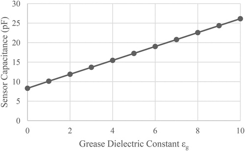
Figure 2 shows a typical change in capacitance as a function of the relative dielectric constant ε_g of the grease. With no grease on the sensor, the calculations provide an estimated capacitance of approximately 8.3 pF with an assumed ε_pcb of 4, which is within a few percent of the measured value. For an increase in ε_g of 1, a corresponding increase in capacitance of 1.78 pF can be measured.

Figure 2. Typical sensor performance.

Heating system

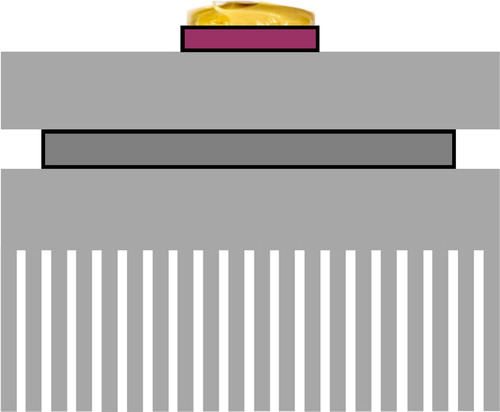
The heating system used in this investigation uses a programmable variable power supply controlled by the same computer that is logging other data. The power supply is connected to a thermoelectric heat pump set up to heat the sensor PCB. A sketch of the heating system with the sensor on top is shown in Fig. 3. The script used to control the instrumentation varies the power provided to the heat pump at a set interval.

Figure 3. Heating system. From top to bottom: sensor with grease sample, aluminum heat spreader, Peltier element (heat pump), and large fan-driven heat sink.

Temperature and capacitance data acquisition

The hardware of the setup is discussed here. The dielectric measurements were taken automatically with a commercially available RCL measurement bridge. Data was automatically recorded to the personal computer (PC) from the RCL bridge using a script. There was no internal averaging set in the instrument to reduce the measurement time, due to sufficiently low noise. The connections between the different components of the measurement system are shown in Fig. 4.

Figure 4. Connection diagram for instrumentation.

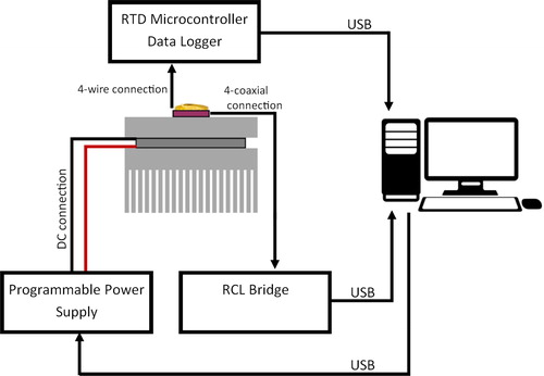
Calibration of the unit was carried out using the measurement cables with connectors that allowed for an open- and closed-circuit calibration with a clean sensor connected. This zero calibration was performed with no grease on the sensor so that the instrument was only displaying the increase in capacitance of the grease samples placed on the sensor surface. The capacitance was recorded from the instrument for this investigation at 90, 900, 9000, and 150,000 Hz. For the purposes of attempting to acquire a correlation with water content, only the capacitance at 90 Hz is used. This frequency was used because it was shown in previous research to have less noise than lower frequencies, to provide a useful correlation with water content, and to not be a multiple of 50- or 60-Hz line frequencies, which could likely cause problems with electrical noise (7). The other frequencies are used only to show the frequency dependence to better understand the behavior of the sensor.

The temperature was logged using a commercially available microcontroller board with a temperature sensor reader.

The measurement procedure and data analysis

There are several steps for preparing a single measurement with one grease sample. After the grease sample is prepared (see third section), it is applied to the surface of the sensor. Assuming the starting temperature of the sensor plate is approximately room temperature, the computer scripts can be started to control temperature and log data.

In this article, a single grease sample measurement series consists of 12 temperature–capacitance cycles acquired over a time frame of 22 hours using a predefined interval to understand the temperature dependence on the capacitance of the grease samples on the sensor and how it changes over time. Immediately upon grease sample application, the 22-hour process is started.

The measured capacitance, C, as displayed in Fig. 2, depends on the dielectric constant, ε_g, of the grease according to Eq. [1][1] $${\mathit{C}}_{\mathit{line}}={\mathit{\epsilon }}_0\left({\mathit{\epsilon }}_{\mathit{pcb}}+{\mathit{\epsilon }}_{\mathit{g}}{\mathit{A}}_{\mathit{g}}+{\mathit{\epsilon }}_{\mathit{c}}{\mathit{A}}_{\mathit{c}}\right)\frac{\mathit{K}\left({\mathit{k}}_1\right)}{\mathit{K}\left({\mathit{k}}_2\right)}+2{\mathit{\epsilon }}_0{\mathit{\epsilon }}_{\mathit{c}}\frac{\mathit{t}}{\mathit{s}}$$[1] and may be modeled as a function of temperature, frequency, water content, sensor coverage, and grease composition. Thus, the measured capacitance can be modeled as [6] $$\mathit{C}=\mathit{C}(\mathit{T},\mathit{t},\mathit{w},\mathit{f},\mathit{A},\mathit{g}),$$[6] where T, t, w, f, A, and g represent temperature, time, water content, frequency, area of sensor coverage, and grease type/composition, respectively. The exact form of this function is unknown and varies between types of grease.

The dielectric thermoscopy method uses the temperature dependence of the capacitance. Thus, it measures how much the capacitance changes for a given temperature change. There are several underlying assumptions of this method:

• The temperature dependence on the capacitance increases significantly with increasing water content.

• The capacitance–temperature slope is linear between reasonable operating temperatures and is immune to absolute temperature.

• Grease coverage on the sensor is repeatable.

• The same trends occur in various types of grease.

With a clean sensor, the capacitance meter has a zero calibration performed before the grease sample is added so that the meter is only displaying the additional capacitance due to the grease sample, instead of the capacitance of the empty sensor.

To acquire a single temperature–capacitance cycle, the sensor (and grease) is heated and cooled in one 15-min cycle temperature sweep from approximately room temperature to around 45 °C using the computer-controlled programmable power supply and a thermoelectric heat pump. The time is divided evenly for heating and cooling. This 15-min cycle is preprogrammed with the scripts running on the PC. The precise time appears to be irrelevant; however, 15 min was chosen because it was estimated to be the realistically shortest time for a machine to heat and cool. The script records N capacitance and temperature measurements during the cycle (in the case of the script used, N = 38), though the exact number is irrelevant if there is sufficiently low noise to acquire the capacitance–temperature slope.

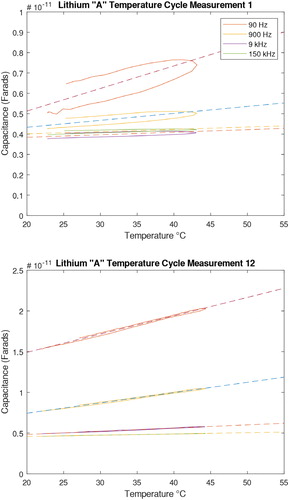
The linear regression from this data is used to represent the capacitance temperature slope of that sample. Figure 5 shows a result from a lithium grease containing 2% water for four different frequencies. Figure 5a plots the capacitance reading as a function of temperature in the first cycle. Figure 5b plots the corresponding capacitance for the last cycle. The dashed lines represent the fit according to Eq. [7][7] $$\mathit{c}=\mathit{Xb}+\mathit{e}$$[7] , and the slope of the line fit represents the capacitance temperature slope: dC/dT (Farads/°C). Hysteresis is initially present but is practically absent after time has passed or several subsequent measurements are made. Based on observation, the hysteresis appears to be based on the total time on the sensor, instead of the temperature cycle. The slope and capacitance have also changed significantly over time, yet normally arrive at a repeatable state after the measurement series is over. It can additionally be observed that lower frequencies change more with temperature, which is primarily why 90 Hz is used instead of a higher frequency.

Figure 5. (a) Top, first measurement, (b) bottom, last measurement. The dashed lines represent linear least squares regression line fits.

The N measurements in a cycle are fitted to the linear model of [7] $$\mathit{c}=\mathit{Xb}+\mathit{e}$$[7] where $\mathit{b}={\left(b_0\mathrm{ }{b}_1\right)}^t$ is the parameter vector, X is an N × 2 system matrix, c is an N × 1 vector of the measured capacitance values, and e is the N × 1 measurement uncertainty vector. The parameter vector b can be solved using the sum of square differences equations.

The variance, V, of the measurement can be quantified as [8] $$\mathit{V}={\mathit{\sigma }}^2=\frac{1}{\left(\mathit{N}-1\right)}\sum _{\mathit{i}=1}^{\mathit{N}}{\mathbf{e}}^2\left(\mathit{i}\right),$$[8] where e = c – Xb and $\sigma$ is the standard deviation of the fit. The main result of this calculation is $b_1=\mathit{dC}/\mathit{dT}$ , which provides the sensitivity of the capacitance measure to a change in temperature for the given variables, T, t, w, f, A, and g. The covariance V_b of b is calculated from the model as ${\mathit{V}}_{\mathit{b}}={\mathit{H}}^{-1}V,\text{ where }\mathit{H}={\mathit{X}}^t\mathit{X}$ and V is the measurement variance given in Eq. [8][8] $$\mathit{V}={\mathit{\sigma }}^2=\frac{1}{\left(\mathit{N}-1\right)}\sum _{\mathit{i}=1}^{\mathit{N}}{\mathbf{e}}^2\left(\mathit{i}\right),$$[8] . Hence, the standard error, ${\sigma }_b$ , of $b_1$ becomes [9] $${\mathit{\sigma }}_{\mathit{b}}=\sqrt{{\mathit{V}}_{\mathit{b}}(2,2)}\mathrm{ }.$$[9]

This represents the error due to noise in the measured data, given the linear model in Eq. [7][7] $$\mathit{c}=\mathit{Xb}+\mathit{e}$$[7] .

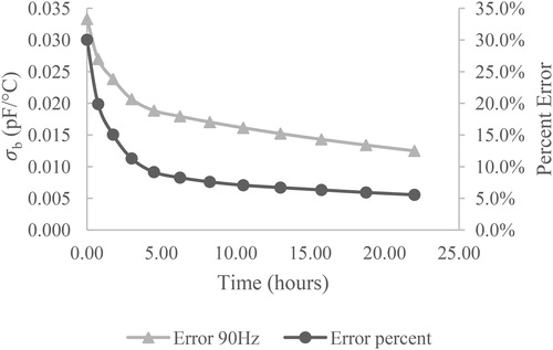
In the case of this experiment, 12 such temperature–capacitance cycles are acquired, which gives 12 estimates of dC/dT and ${\sigma }_b$ , respectively, with a set duration of 22 hours between the first and last measurements. The evolution of ${\sigma }_b$ for the 90 Hz frequency is shown in Fig. 6 for a representative grease sample. As can be seen in the plot, the total error present in the linear models approaches a constant value of roughly 0.01 pF/°C, or equivalently 5% of the dC/dT.

Figure 6. Evolution of total error (gray triangles) and relative error (black circles) over an extended measurement period.

Additional errors for the estimate of dC/dT come from uncertainties in estimating the water content of the grease mixing process, ${\sigma }_m$ (as found in previous measurements from (6)), and errors from the measurement repeatability, ${\sigma }_r$. For the purposes of this experiment, the intended water content is assumed to have a 5% error. Thus, ${\sigma }_m=\frac{\mathit{dC}}{\mathit{dT}}\times 0.05$ for the given linear regression. A typical value is in the order of 0.01 pF/°C, which is in the same range as ${\sigma }_b$. The value ${\sigma }_r$ represents the repeatability of the measurement. Using the same grease sample of a 1% wate-contaminated sample of CaS-X “A,” five measurements were made giving a standard deviation of 0.0034 pF/°C, and this is assumed to be representative of a reasonable repeatability error for all other grease samples. As a conservative estimate, ${\sigma }_r$ is set to 0.0034 pF/°C for the remainder of this article. Finally, the total error is $\sigma =\sqrt{{\sigma }_b^2+{\sigma }_m^2+{\sigma }_r^2}$, assuming the three error sources to be uncorrelated and Gaussian distributed. In the remainder of the article, the error bars are displayed as ±$\sigma \mathrm{ }$ unless otherwise noted.

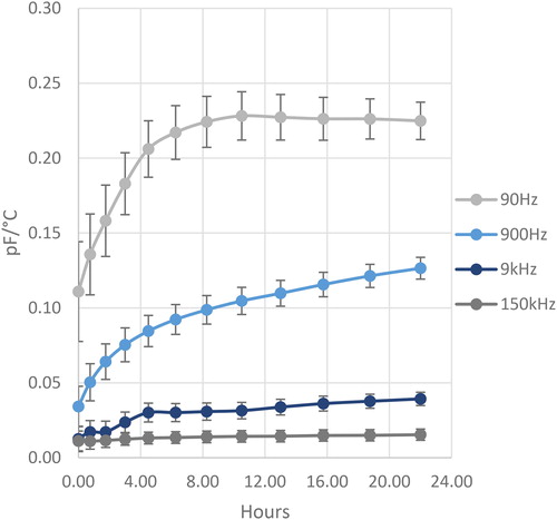
The estimates of dC/dT over a complete measurement series for a representative measurement of a lithium grease with approximately 2% added water and for the different frequencies are summarized in Fig. 7 together with the error estimates. It can be seen that there is a certain settling time for all frequencies, where all frequencies display an asymptotic behavior. It is further seen that the sensitivity for a change in temperature is significantly larger for the low frequencies as compared to the higher frequencies and that the random errors decrease with time. In the remainder of this article, a measurement for a certain grease type with a certain water content is therefore measured at 90 Hz and is taken as the average of the last four measurement points in the measurement series of 12 measurements.

Figure 7. Example of lithium grease “A” with 2% added water. The lower frequencies have a much larger dependence on temperature.

Experiments

This section first outlines the grease types used and how the samples were prepared for the experiments in this paper. The results from this investigation are then summarized.

Water-contaminated grease sample preparation

The greases examined in this investigation are shown in Table 1. Two common and reputable brands of calcium sulfonate complex (CaS-X) and three plain lithium (Li) greases were used to verify how the sensor functions when two manufacturers produce the same type of grease. Additionally, one type of lithium complex (Li-X) grease was used. All new greases were measured with a Karl-Fischer titration instrument to quantify their initial water content. This is necessary because it cannot be assumed that all new greases contain essentially no water.

Table 1. The greases used in this experiment.

Grease	Thickener	Base oil
CaS-X-A	Calcium sulfonate Complex (brand “A”)	PAO + mineral
CaS-X-B	Calcium sulfonate Complex (brand “B”)	Unknown
Li-A	Lithium (brand “A”)	Mineral
Li-B	Lithium (brand “B”)	Mineral
Li-C	Lithium (brand “C”)	Mineral
Li-X	Lithium complex	Mineral
Plain-Li*	Lithium	PAO

* This grease is unadditivized.

Additionally, a set of 7 samples of the CaS-X Brand “A” was made with small quantities of added water up to 0.97% to characterize the sensor and how well it can measure small changes in water content.

The grease mixing setup is comprised of two syringes connected end to end with a short length of vinyl tubing such that they are sealed and airtight. The mixing method has been previously described in (9). Other mixing methods are probably suitable, assuming the mixture is sufficiently homogenized.

Table 2 shows the water content in the samples used in the experiment. The range in quantity of water was chosen because several drops of added water ended up increasing the water content of the 30-g sample of grease by approximately 0.3%. This was thought to be a rational starting point, as many bearings can contain that order of magnitude of grease and several drops of water subjectively seemed like a reasonable quantity to be able to distinguish, since this amount could easily be caused by either water ingress or condensation from heating and cooling cycles. The amount was increased arbitrarily until it was apparent that the saturation point of the grease was surpassed and the visible appearance changed. Also, anything higher than the ∼5% water content of the most contaminated samples would likely not be useful information, as it is already a very significant level of contamination and bearing damage could follow shortly.

Table 2. Water content of grease samples.

Grease sample	Added water	Total water
CaS-X-A New	—	0.31%
1	0.14%	0.44%
2	0.49%	0.80%
3	0.47%	0.78%
4	0.78%	1.09%
5	1.54%	1.85%
6	2.83%	3.14%
7	5.10%	5.41%
CaS-X-B New	—	0.19%
1	1.03%	1.22%
2	2.50%	2.69%
3	5.56%	5.75%
Lithium-A New	—	0.060%
1	1.96%	2.02%
2	3.10%	3.16%
3	4.68%	4.68%
Lithium-B New	—	0.055%
1	1.20%	1.25%
2	2.51%	2.56%
3	5.44%	5.49%
Lithium-C New	—	0.05%
1	5.28%	5.33%
Li-X New	—	0.040%
1	2.83%	2.87%
2	5.0%	5.04%
Plain Li	—	0.01%
1	1.27%	1.28%
2	2.51%	2.52%
3	4.85%	4.86%

Note. Values are given in weight percent. Added water content is assumed to be ± 2.5% of the value given.

Table 3 specifies the water content of the samples used to characterize the capabilities of resolving small changes in water content. A large sample of CaS-X-A was made (with approximately 0.97%) and was fractioned appropriately with new grease to arrive at the water content in the table. The same mixing method was used, albeit with small 10-ml syringes, sized for the small samples used. Fractioning the 0.97% added water sample with new grease was required because the amount of water was so small it would have been impractical to be consistent due to human and measurement errors.

Table 3. Water content for low water content experiment with CaS-X (Brand “A”) samples.

CaS-X “A”	Added water	Total water
0	0%	0.31%
1	0.10%	0.41%
2	0.24%	0.54%
3	0.38%	0.69%
4	0.54%	0.85%
5	0.66%	0.97%
6	0.81%	1.12%
7	0.97%	1.28%

Note. The total water content is higher due to the comparatively high water content of the new grease. Added water content is assumed to be ±2.5% of the value given.

Results

Each of the 29 samples in Table 2 and the 8 samples in Table 3 were measured during the 22-hour sequence specified in the second section. The data from the low water content measurement of the CaS-X Brand “A” Table 3 are compiled in Fig. 8. The results show a linear increase in the DT measurement with a slope ranging from 0.13 pF/°C to 0.19 pF/°C for an increase in water content from 0.31% (new) to 1.27% with sufficient resolution and low enough noise in the capacitance and temperature measurements to be able to determine small differences in water content.

Figure 8. Data compiled from all eight CaS-X brand “A” low water content samples.

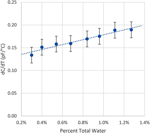
The rate of increase in the DT measurement for CaS-X “A” corresponds to an estimated 0.54 pF/(10 °C-%w). This value represents a 0.54 pF increase in capacitance for a change of 10 °C and increase of 1% water in this experiment.

Figure 9 presents the data for all the tested greases as a function of water content. Note that it is theoretically possible for the slope to be slightly negative with a very dry material of low dielectric constant. This is likely due to the comparatively low dielectric constant and nonpolar properties of the greases. As the grease heats up, the thermal expansion is more than the change in dielectric constant. The slope measures α = d²C/dTdw, where C, T, and w represent the capacitance, temperature, and water content (in weight percent), respectively, are summarized in Table 4.

Figure 9. The dC/dT dependence as function of water content for all tested greases from this investigation.

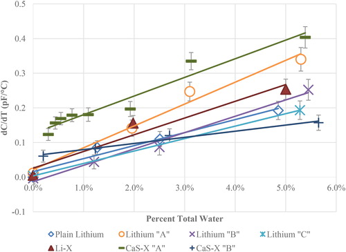
Table 4. The slopes of the lines in Fig. 9.

Grease	α (pF/10 °C-w%)
Lithium “A”	0.631 ± 0.032
CaS-X “A”	0.537 ± 0.025
Li-X	0.482 ± 0.025
Lithium “B”	0.472 ± 0.028
Lithium “C”	0.359 ± 0.028
Plain Lithium	0.375 ± 0.025
CaS-X “B”	0.173 ± 0.021

Of the tested greases, two have a slightly different behavior than the others, though all show a clear increase in the measurement with increasing water. This lithium “A” was subjectively more challenging to mix with water and was observed to be more hydrophobic. This difference from the other greases could indicate that water is rejected from the water–grease mixture to the surface of the sensor causing a disproportionate amount of water to be measured. The relationship between the DT measurement and water content has a trend that essentially approaches the origin of the plots for all the tested lithium-based greases.

Also, in Fig. 9 it can be observed that the two CaS-X greases have a different behavior than the lithium greases. The CaS-X greases do not approach the origin of the plots but have an offset above the x-axis. CaS-X “A” and “B” have an offset of approximately 0.12 and 0.06 pF/°C, respectively, which is more than any of the other greases.

It is unclear why the two CaS-X greases in this plot have a similar DT relationship with water content with a different offset in the y-axis. This could be due to yet unknown grease components whose dielectric properties have a similar relationship to water content. It should be noted that the CaS-X “A” and “B” greases have been measured with a Karl-Fischer titration instrument and shown to contain 0.31 and 0.19% water, respectively, even when new. This is already considered in the plots. More research will have to be done to understand why these differences are observed. It should be noted, however, that regardless of the type of grease used, an increase is always observed, and the benefits of the DT method still otherwise apply.

Discussion and conclusion

In this article, a method called dielectric thermoscopy was investigated with multiple greases with a homogenized water content ranging from 0 to approximately 5% and one grease between 0% and 0.97% in multiple steps. The automated measurement was shown to be consistent and accurate using the interdigited fringe field capacitor plate. Since the method previously functioned using larger test cell/sensor configurations (7), the latest measurements in this study only show additional promise to work in an application. The automated measurement aspect of this article appears to be a success and shows further promise with future development.

The custom-made sensor used in this experiment is shown in Fig. 1. The size was chosen based on the calculations in the second section to be the smallest possible while still having a measurable capacitance with sufficiently low noise using the measurement equipment available. There was an evolution with the sensors where certain design characteristics were found to not work. If the separation distance was too small, it appeared that small droplets within the grease would “short” the sensor. Polymer coatings and metal oxide films were also tested but they either introduced significant dielectric properties to the sensor or ostensibly caused incompatibilities with some greases due to the difference in hydrophobicity between the greases and coatings. Future research will have to be done to understand whether coatings will help the sensor.

Twelve measurements of a complete heating and cooling cycle are taken over the period of 22 hours for each prepared grease sample. Averaging the last four measurements appeared to give the most reliable set of data. The exact time of each measurement and between each measurement does not appear to influence the quality of the data, though since everything is logged automatically on the PC, the intervals are set to make each set of measurements as reproducible as possible and reduce the influence of human error. An example of this data is shown in Fig. 7. It is observed that the measurements at lower frequencies are far more sensitive to a change in water content as compared to the higher frequencies. The reason for this can be coupled with the dielectric properties of water. While the real component of the dielectric constant ($\epsilon \mathrm{\text{'}}$ ) of water can be approximated to 78 for most frequencies above 1 MHz (10), the low-frequency properties are far different. As the frequency is reduced below the range of kilohertz, the dielectric constant increases dramatically due to the formation of dipoles (11) and the ability of the protons to migrate distances larger than the normal dimensions of water molecules, thus increasing conductance (10). Fundamental research on the physical chemistry of water has shown interesting results (12). Even for filtered water, it was revealed that ${\epsilon }^{\mathrm{\text{'}}}$ can be as high as 2 × 10⁶ at 100 Hz, but drops to around only 400 at 4 kHz and 28 °C. This is primarily due to the electrode polarization from the aforementioned proton migration causing electrode polarization with an electric field of greater than 100 V/m (13). In the case of this sensor with a measurement voltage of 1.5V and a separation distance of 1 mm in the fringe field sensor, the electric field is 1500 V/m. Low frequencies have an advantage of having an ${\epsilon }^{\mathrm{\text{'}}}$ value of orders of magnitude higher than the typical higher frequencies used in dielectric measurements, in addition to the temperature dependence used in this dielectric thermoscopy method. A brief background was further described in a previous paper (7).

As a further observation in Fig. 7, there is a certain amount of “settling” in the measurement of the sensor, where it increases and stabilizes to a relatively stable value after around 8 hours. As displayed in Fig. 5, it was often observed that the first few measurements after grease application have a significant amount of hysteresis in the capacitance measurement as the sensor and grease cools back down. The grease appears to “settle” on the surface and change the measurement over time, due to unknown reasons. The hysteresis essentially disappears once the measurement stabilizes if no other problems are present. One known problem is when a water droplet is “shorting” the traces on the surface of the sensor, which increases the conductance of the sensor and greatly exaggerates the water content. For the purposes of a sensor meant to detect damaging water in a machine, this is not likely an issue since droplets of water are significantly worse for the machine than if it were homogeneously mixed within the lubricant. The greases that were observed to be significantly more hydrophobic (i.e., more difficult to mix properly) caused more problems in the measurement and would take longer to “settle” on the sensor or would never reach a steady-state value. This was attributed to large droplets forming a disproportionate amount on the surface of the sensor. Since this is a surface problem, other capacitive sensor embodiments with larger distances between the sensing elements could remedy this problem.

Each grease appears to have a different settling behavior, with no obvious correlation to the type of grease or amount of water contamination (though all new greases have essentially no settling time). Most well-prepared samples will settle to a constant value after 2–8 hours. it is worth noting that subjectively, the limitation of this experiment was in sample preparation, instead of the measurement itself. There are many components to the grease mixture, and manufacturers are secretive about what they contain. Observationally, even though there is no clear correlation, the quantity of water contamination has a role. It was experimentally observed that new greases settle within a short time, often within the first several measurements. Some greases with 5% added water may require a significant time to approach a steady value. This could be due to the water not being stationary in the mixture, or water droplets forming on the surface of the sensor due to differences in the hydrophobicity of the grease and surface of the sensor. One possible explanation to this settling observation is that the AC electric field used in the sensor, though only 1.5 V RMS, is high enough at 1500 V/m to coalesce water droplets if the water and grease have surface tension properties that encourage such behavior (14), causing the measurement to change over time. Presumably, the polarity of the grease constituents could play a role as well, as that changes the ability of any mixture to hold onto water.

It was desired to test multiple greases to characterize the measurement method and verify what problems could occur once the grease type is included as a variable. It was shown that all tested greases respond with a linear increase in the DT measurement with an increase of water content; however, some greases increase at a different rate. The results show that the lithium greases all perform in a similar fashion, with one moderate outlier. They all start at very close to dC/dT = 0 for a water content of 0% and then increase in proportion to the water content. The outlier (lithium “A”) was subjectively harder to mix with water, which might cause water to be rejected to the surface of the sensor, causing a disproportionately large amount of water to form where the sensor is most sensitive. The nonlithium greases, calcium sulfonate complex, have a different behavior with a slight positive offset, with the second grease having a much lower increase to the DT measurement for the same increase in water content. Part of the reason is that they have up to 0.3% water when new, while the lithium greases tested do not. The increase in the DT measurement with increasing water is also following a different slope. The reasons for this are not known. The CaS-X greases were subjectively far easier to mix with large quantities of water, as was observed in the literature (4). In connection to the very hydrophobic lithium grease, a possible explanation is that this CaS-X grease might absorb water so well that the sensor surface has a comparatively lower amount of water to be measured. Otherwise, differences in chemistry might influence this measurement.

Between the water content range of 0% and approximately 5% water, the dielectric thermoscopy measurement provided a useful correlation to water content with the chosen frequencies in the measurement. The average sensor response of all tested greases is 0.44 pF for a temperature change of 10 °C and an increase in water content of 1%. The standard deviation is 0.15 pF. With the CaS-X “B” grease removed, the average sensor response becomes 0.48 pF for a temperature of 10 °C and an increase in water content of 1%, with a standard deviation of 0.10 pF. The correlation is likely good enough to be able to develop a model in the future, although different greases behaved in a different way, likely requiring calibration data for different applications.

Additional information

Funding

This work is partially supported by the SKF–LTU University Technology Center (UTC) and the Jacob Wallenberg Foundation. The authors gratefully acknowledge SKF and the Jacob Wallenberg Foundation for support that has made possible the initiation of this research in advanced condition monitoring techniques within LTU.

References

- Mobley, K. (2002), An Introduction to Predictive Maintenance, 2nd ed., pp. 23–42, Elsevier Science: Woburn, UK.
- Hong-Bae, J., Kiritsis, D., Gambera, M., and Xirouchakis, P. (2006), “Predictive Algorithm to Determine the Suitable Time to Change Automotive Engine Oil*,” Computers & Industrial Engineering, 51, p. 671.
- Schnabel, S., and Larsson, R. (2014) “Study of the Short-Term Effect of Fe3O4 Particles in Rolling Element Bearings: Observation of Vibration, Friction and Change of Surface Topography of Contaminated Angular Contact Ball Bearings,” Proceedings of the Institution of Mechanical Engineering Part J—Journal of Engineering Tribology, 228, pp. 1063–1070.
- Cyriac, F., Lugt, P. M., and Bosman, R. (2016). “Impact of Water on the Rheology of Lubricating Greases,” Tribology Transactions, 89, pp. 679–689.
- Siebert, H., and Mann, U. (2005), “Gear Oils Based on Polyglycols—New Solution for the Lubrication of Large Industrial Gear Drives,” Proceedings of the World Tribology Congress III—WTC.
- Dittes, N. (2016), “Condition Monitoring of Water Contamination in Lubricating Grease for Tribological Contacts,” Licentiate Thesis, Luleå University of Technology, Luleå, Sweden.
- Dittes, N., Pettersson, A., Defeng, L., and Lugt, P. M. (2017), “Dielectric Thermoscopy Characterization of Water Contaminated Grease,” Tribology Transactions, 61, pp. 393–402.
- Abu-Abed, A. S., and Lindquist, R. G. (2008), “Capacitive Interdigital Sensor With Inhomogeneous Nematic Liquid Crystal Film,” Progress in Electromagnetics Research B, 7, pp. 75–87.
- Dittes, N., Pettersson, A., Lugt, P. M., Sjödahl, M., and Casselgren, J. (2018), “Optical Attenuation Characterization of Water Contaminated Grease,” Tribology Transactions, 61, pp. 726–732.
- Fernández, D. P., Mulev, Y., Goodwin, A., and Levelt Sengers, J. M. H. (1995), A Database for the Static Dielectric Constant of Water and Steam, vol. 24. Available at: https://aip.scitation.org/doi/10.1063/1.555977
- Lewowski, T. (1998), “Dipole and Induced Electric Polarization of Water in Liquid and Solid Phase: A Laboratory Experiment,” American Journal of Physics, 66, pp. 833–835.
- Angulo-Sherman, A., and Mercado-Uribe, H. (2011), “Dielectric Spectroscopy of Water at Low Frequencies: The Existence of an Isopermitive Point,” Chemical Physics Letters, 503, pp. 327–330,.
- Cole, R. H. (1989), “Dielectrics in Physical Chemistry,” Annual Review of Physical Chemistry, 40, pp. 1–29.
- He, L., Yang, D., Gong, R., Ye, T., Lü, Y., and Luo, X. (2013), “An Investigation into the Deformation, Movement and Coalescence Characteristics of Water-in-Oil Droplets in an AC Electric Field,” Petroleum Science, 10, pp. 548–561,.