Assessment of wind shelter conditions of an open water storage reservoir using wind shelter index

Abstract

Sharifi MR, Shahi Z. 2020. Assessment of wind shelter conditions of an open water storage reservoir using wind shelter index. Lake Reserv Manage. XX:XXX–XXX.

Identifying the wind-affected area in a given waterbody facilitates the implementation of some evaporation control methods because the amount of evaporation is a function of the wind shelter. In this study, a method is developed to identify the wind-affected area of open water in reservoirs, using the Dez Dam in Iran. Through the wind shelter index (Sx), which is most commonly used in snowy areas, the wind shelter was calculated at different points on the open water. The points were then categorized in terms of the wind shelter index values using cluster analysis. For this purpose, Sx values were calculated and then clustered using 28,321 points of the lake’s surface. Using this method, the water surface was classified into areas, with 5 parts having different wind sheltering. On average, a considerable part of the water surface of the lake (66%) was more exposed to the wind than other parts. Therefore, it can be predicted that the evaporation at these areas is higher than at other areas of the lake surface.

Keywords:

• Cluster analysis
• evaporation control
• free-surface evaporation
• wind shelter index

One of the most effective water loss processes in dams is evaporation from the open water. In some cases, evaporation rates are higher than water use in these systems (Gokbulak and Ozhan 2006). Iran is one of the arid to semi-arid countries where evaporation from open water is high, with an average annual evaporation rate of 195 mm, accounting for 72% of the average annual precipitation (Sarang 2001). Methods to reduce water loss through evaporation, especially in arid regions such as Iran, are thus of great importance. Many countries, including the United States, Australia, India, Turkey, and Canada, use evaporation control methods to reduce water losses stored in reservoirs (Barnes 2008). The main techniques involve physical and chemical methods; biological methods, such as using aquatic plants to cover the surface of the water and prevent evaporation, are not widely used. Each of these methods, depending on the conditions in which they are used, will prevent a different degree of evaporation (Cluff 1977, Jennison 2003, Craig 2005, Craig et al. 2005, Craig et al. 2007, Barnes 2008, Vara-Orta 2008, Choi 2014). In chemical methods, monolayers (usually cetyl or stearyl alcohol or a mixture of these) are used and are usually dispersed by wind (Jennison 2003). Physical methods such as floating coatings, floating balls, and solar panels can withstand winds at speeds of 70–170 km/hr (Vara-Orta 2008, Choi 2014). Hence, the use of these methods is appropriate for controlling evaporation from the surface of the water in windy areas.

Points on the earth’s surface receive different amounts of wind energy, in part due to the surrounding topography. Wind moving from the mountains to the lowlands downstream reduces its speed and thus reduces the kinetic energy reached in these lowland areas. In recent years, many studies have quantified the effects of terrain on wind patterns. A measure to quantify this energy is the wind shelter index (Sx). The definition of the Sx is taken from the solar shading phenomenon on the horizon, made of some high altitudes in radiation modeling (Dozier et al. 1981). In fact, the Sx of a point is estimated based on the wind-blowing slope between the mentioned point, its upwind point, and the wind-blowing stream. This slope is called the upwind slope.

Winstral et al. (2002) developed Sx by studying the spatial variation of snowpack accumulated under wind influence. Since then, various researchers have used this index to study snow behavior. Because the importance of the wind factor has been proven in many processes, including evaporation, some researchers have used the Sx in nonsnowy conditions (Winstral et al. 2009, Farokhzadeh et al. 2014). For example, Farokhzadeh et al. (2014) developed an algorithm that calculates Sx without the need for snow height and compared their results with the research of Sharifi (2007). Sharifi (2007) had obtained Sx values in a snowy area using the Winstral et al. (2002) method. In general, most studies for determining the wind shelter index of different areas either need a ground measurement of wind speed, which usually has a high cost, or are only useable in snowy locations (Winstral et al. 2002, Erickson et al. 2005, Molotch et al. 2005, Molotch and Bales 2006, Sharifi et al. 2007, Litaor et al. 2008, Tabari et al. 2010, Winstral et al. 2009, Maroufi et al. 2010).

One of the steps in calculating the Sx is determining the effective length of the wind shelter. The choice of effective length varies according to the type of Sx application. For example, in some studies carried out in snowy areas, the effective length is selected so that its corresponding Sx has higher correlations than other lengths with the depth of the snow at the points where Sx is calculated (Winstral et al. 2002, Erickson et al. 2005, Molotch et al. 2005, Molotch and Bales 2006, Sharifi et al. 2007, Litaor et al. 2008, Tabari et al. 2010, Maroufi et al. 2010). Moreover, considering the application of Sx in nonsnow conditions (Farokhzadeh et al. 2014), and the impossibility of examining and comparing the correlation between Sx and snow depth, other criteria have been used to select the effective length in nonsnow areas. For example, Farokhzadeh et al. (2014) used an average wind shelter slope parameter to determine the effective length. Meanwhile, the Winstral et al. (2009) method needed a large web of wind sensors for measuring the wind speed in different places.

Given the development of evaporation control methods on the surface of open water, the present study aims to assess wind shelter conditions at different parts of a reservoir’s surface to determine the areas that are most exposed to evaporation due to wind. The development of a method to divide the reservoir surface according to wind shelter conditions could be a useful tool to optimize the costs of evaporation control methods. It could also help water resource managers evaluate the efficiency of a wind shelter in reducing evaporation or for coupling with hydrodynamic models.

Study area

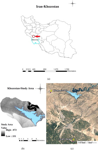
In this study, we investigated the wind shelter conditions at the surface of a reservoir. The lake of Dez Dam, located at latitude 32°35′45′′ to 32°43′38′′ N and longitude 48°18′51′′ to 48°30′20′′ E, has a basin area of ∼60 km². The surrounding topography is mountainous, with elevations ranging from 331 to 873 m (Figure 1), making it an appropriate area in which to study the effect of altitude on the amount of Sx on the lake surface.

Figure 1. The locations of the study areas: (a) the location of the study area in Iran and Khuzestan province, (b) elevations overlooking the lake (m), and (c) the locations of Hosseinieh and Safi Abad synoptic stations in relation to Dez Dam Lake.

Materials and methods

Time period

The value of the Sx parameter depends on the points being examined. In this study, the height of points is equal to the water level. Therefore, the average monthly water level height for the period 2011–2016 was considered as the elevation of the studied points. Also, since the application of Sx in evaporation is of interest in this study, June, July, August, and September were selected as the months examined, since in this study area these are the hottest months of the year, when the probability of evaporation is high.

Prevailing wind direction

The prevailing wind direction (i.e., the most common wind direction with the highest speed) must be determined to calculate Sx in the study area (Winstral et al. 2002). In general, due to the low spatial variation of wind direction, the prevailing wind direction of a meteorological station can also be extended to adjacent areas. Therefore, to determine the prevailing wind direction in the Dez Dam area, wind direction and wind speed data were used from 2 synoptic stations of Hosseinieh and Safi Abad, which are located 13 and 38 km from Dez Dam, respectively. Given that the wind data for these 2 stations were the only information available in the region, the arithmetic mean for the prevailing winds of these 2 stations (292.5°) was used as the prevailing wind direction for the Dez Dam area.

To determine the direction of the prevailing wind, after providing hourly data of wind speed and direction for 2 stations for the 2005–2016 period, the monthly wind rose diagrams for June, July, August, and September were plotted for both stations using WRPLOT View software, which calculates the frequency of wind at different speeds and directions. An angular tolerance of 60° for the prevailing wind direction was applied to account for wind direction fluctuations (Elder 1995, Winstral et al. 2002, Erickson et al. 2005). Therefore, since this range includes azimuths for the prevailing wind direction of both Hosseinieh (270°) and Safi Abad (315°) stations, it can be expected that the prevailing wind direction used for the Dez Dam area is very similar to reality.

Wind shelter index (Sx)

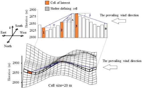
The concept of wind shelter is based on the phenomenon of sunlight shadowing on the horizontal surfaces by solar radiation modeling (Berg 1986). Selecting a maximum shelter-producing pixel based on the slope is analogous to the determination of solar shading within the horizon function used in radiation modeling by Dozier et al. (1981). This was calculated as the amount of radiation received at each point in the grid for different solar angles. Sx is calculated by determining the gradient of the wind between a given point and the point located upstream of it along with the wind direction. This gradient is called the wind opposing or facing gradient (Winstral et al. 2002). In defining the wind shelter index, the angles over the horizon line are positive (wind shelter) and the angles under the horizon line are negative (exposed to wind; Figure 2). The situation of the wind shelter at 3 points 1, 2, and 3, which are against the direction of the prevailing wind direction (from right to left), shows that the upward slope of points 1 and 2 is positive (α and γ) and the effective altitude in its wind shelter is altitude A, but point 3, with a negative upwind slope (β), is exposed to wind and the effective altitude in its wind shelter is altitude B (Figure 2). Sx is calculated based on the prevailing wind direction and topography of the region (Winstral et al. 2002): (1) $${Sx}_{A,\mathit{dmax}}\left(x_i,y_i\right)=\mathit{max}\left[\hspace{0.17em}{\text{tan}}^{-1}\left(\mathit{ELV}\left(x_v,y_v\right)-\mathit{ELV}(x_i,y_i)/{\left[{(x_v-y_v)}^2+{(x_i-y_i)}^2\right]}^{0.5}\right)\right]$$(1) where Sx is the maximum wind-facing gradient (in degrees), A is the azimuth of the direction considered for Sx calculation, which is the same as the wind direction (in degrees), d_max is the maximum selected length in the upward direction (in meters), ELV is the elevation (in meters), x_i and y_i are the coordinates of the considered point (UTM), and x_v and y_v are the coordinates of the points located along A and up to the maximum distance dmax from the considered point.

Figure 2. Schematic view of the wind shelter situation, with 3 points (1, 2, and 3) based on a linear profile from a hypothetical topography (Winstral et al. 2002, Farokhzadeh et al. 2014).

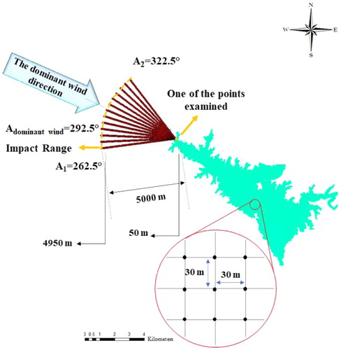
To calculate Sx at any point, a sector (referred to as a sector or impact range) with a central angle of Ө degrees is considered on the point of interest where the prevailing wind direction in the region passes through the center of the sector. This sector is considered in order to observe oscillations of the prevailing wind direction. According to Winstral et al. (2002), Ө = 60° was considered. Then, to investigate the effect of all elevations within the impact range on the wind shelter rate of the points, the sector is divided into 13 directions with an angular distance of 5° (60° in total) and the number of points located within the range of influence is determined for the directions. Afterward, the coordinates of the points in the influence are determined from equations 2(2) $$X_v=X_i+d_{\mathit{max}}\text{cos}\mathrm{\alpha }$$(2) and 3(3) $$Y_v=Y_i+d_{\mathit{max}}\text{sin}\mathrm{\alpha }$$(3) : (2) $$X_v=X_i+d_{\mathit{max}}\text{cos}\mathrm{\alpha }$$(2) (3) $$Y_v=Y_i+d_{\mathit{max}}\text{sin}\mathrm{\alpha }$$(3)

where X_v and Y_v are the coordinates of the points located in each direction, X_i and Y_i are the coordinates of the measurement points, and α is the azimuth angle of the prevailing wind direction. Sx is obtained by applying equation 1(1) $${Sx}_{A,\mathit{dmax}}\left(x_i,y_i\right)=\mathit{max}\left[\hspace{0.17em}{\text{tan}}^{-1}\left(\mathit{ELV}\left(x_v,y_v\right)-\mathit{ELV}(x_i,y_i)/{\left[{(x_v-y_v)}^2+{(x_i-y_i)}^2\right]}^{0.5}\right)\right]$$(1) to the number of points on the impact range of each of the considered points. In the present study, the accuracy of the area’s topographic map was 25 m, based on a digital elevation model (DEM) map prepared to a 1:25,000 scale. Proportional to the accuracy of the DEM, a 30 m × 30 m grid containing 28,321 points was placed on the DEM of the dam lake to analyze the wind shelter. The goal was to calculate the value of Sx at 28,321 points on the surface of the water. By examining the distance between the points of the network and the elevations overlooking the wind-facing margin of the lake, it was observed that the points closest and farthest to these elevations were located at a distance of 50 m to 5000 m, respectively. Therefore, the wind shelter values at all points of the grid, using equations 2(2) $$X_v=X_i+d_{\mathit{max}}\text{cos}\mathrm{\alpha }$$(2) and 3(3) $$Y_v=Y_i+d_{\mathit{max}}\text{sin}\mathrm{\alpha }$$(3) , were calculated at maximum distances (d_max) of 50, 100, 150, 200, 250, …, 49,505,000 m (101 lengths with distances of 50 m).

At each studied point, 1313 (101 lengths × 13 directions) values were calculated for Sx using equation 1(1) $${Sx}_{A,\mathit{dmax}}\left(x_i,y_i\right)=\mathit{max}\left[\hspace{0.17em}{\text{tan}}^{-1}\left(\mathit{ELV}\left(x_v,y_v\right)-\mathit{ELV}(x_i,y_i)/{\left[{(x_v-y_v)}^2+{(x_i-y_i)}^2\right]}^{0.5}\right)\right]$$(1) . Hence, we have a large number of Sx values at each point. One of the steps in solving this problem is to calculate the average Sx. The average Sx should be calculated for a number of selected lengths that reflect the wind situation in the study area well (Winstral et al. 2002). In this study, according to the topographic conditions around the lake and the distance and proximity of the points to the elevations overlooking the wind-facing margin of the lake, from the closest d_max to farthest d_max, the lengths of 50, 100, 200, 300, 500, 1000, 1500, 2000, 3000, 4000, and 5000 m were selected. Assuming that they could describe the wind shelter in the study area well, the average Sx values were calculated using equation 4(4) $${\overline{Sx}}_{\mathit{dmax}}\left(x_i,y_i\right)|\begin{array}{c}{A}_2\\ A_1\end{array}=1/n_v\sum _{A=A_1}^{A_2}{Sx}_{A,\mathit{dmax}}(x_i,y_i)$$(4) for these lengths (Winstral et al. 2002). That is, the average of the 13 calculated Sx values, corresponding to these 11 lengths, in 13 different directions, was calculated: (4) $${\overline{Sx}}_{\mathit{dmax}}\left(x_i,y_i\right)|\begin{array}{c}{A}_2\\ A_1\end{array}=1/n_v\sum _{A=A_1}^{A_2}{Sx}_{A,\mathit{dmax}}(x_i,y_i)$$(4) where n_v is the number of directions defined in the impact range located between azimuths A₁ and A₂ degrees (13 numbers) with a d_max radius. Sx values were calculated at each point using an algorithm prepared using MATLAB software.

Calculating the Sx for these lengths does not mean that the effect of the rest of the lengths on the wind shelter at any point is ignored. Since the ultimate goal is to achieve a unique value of Sx at every point in the study area, it is necessary to calculate a single distance called the effective length of the wind shelter.

Determining the effective length

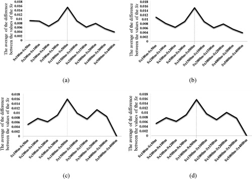
To determine the effective length in this study, the differences between Sx values corresponding to the points at both maximum selected lengths were examined. Variations in the average difference in Sx were plotted as defined points in both consecutive lengths for each of 10 successive changes of 50 to 100, 100 to 200, 200 to 300, 300 to 500, 500 to 1000, 1000 to 1500, 1500 to 2000, 2000 to 3000, 3000 to 4000, and 4000 to 5000 m. That is, Sx₁₀₀ – Sx₅₀, Sx₂₀₀ – Sx₁₀₀, …, Sx₄₀₀₀ – Sx₃₀₀₀, and Sx₅₀₀₀ – Sx₄₀₀₀ were calculated for all points. Given the effective length applied for choosing the most effective elevation for the wind shelter of the points, the length for which the corresponding elevation creates the greatest difference in the wind shelter rate was chosen as the effective length of the study area. After examining the average values of the wind shelter differences in both sequential lengths, the accuracy of this point was observed in the range of 500 to 1000 m. Therefore, the distance of 1000 m was chosen as the effective length and the corresponding Sx values were used as wind shelter values at the considered points.

Validation and sensitivity analysis

To assess Sx variations among the selected months, the average wind shelter values of points were determined for each month. Since points near the lake’s margin are influenced more by surrounding topography than by points farther from shore, it should be expected that wind shelter will be greater along shorelines than in open water. As a result, the average wind shelter values were investigated each month in 2 groups of points facing the wind, the margin and central subareas of the lake.

To perform the sensitivity analysis of Sx values to changes in monthly water level, the average changes in Sx were calculated using equation 5(5) $$\text{Average changes in} Sx=\sum _{i=1}^n\left[\left(\frac{{Sx}_2-{Sx}_1}{{Sx}_1}\right)100\right]/n$$(5) for each of the months studied and were compared with the corresponding values in the preceding month: (5) $$\text{Average changes in} Sx=\sum _{i=1}^n\left[\left(\frac{{Sx}_2-{Sx}_1}{{Sx}_1}\right)100\right]/n$$(5) where n is the number of points in the network, Sx₂ is the Sx value in the month under study, and Sx₁ is the Sx value in the previous month.

Changes in the lake water level were calculated for every 2 consecutive months using equation 6(6) $$\text{Changes in lake water level}=({\mathit{WSE}}_2-{\mathit{WSE}}_1)/\Delta H\times 100$$(6) : (6) $$\text{Changes in lake water level}=({\mathit{WSE}}_2-{\mathit{WSE}}_1)/\Delta H\times 100$$(6) where ΔH is the difference between the highest water level and the lowest water level during the months studied and WSE₂ – WSE₁ shows the difference in average water level of each month compared to the previous month. Thus, by comparing the differences of Sx in the months resulting from the variation of the water level of the lake, one can examine the sensitivity of Sx to water level changes.

Cluster analysis

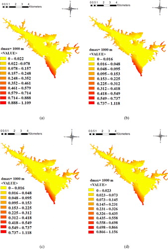
To make Sx values discernible on the surface of the lake, cluster analysis was performed using the K-means (Habibi 2015) and Ward (Gong and Richman 1995) hierarchical clustering methods in SPSS 22 software. To perform the K-means method in this software, the number of clusters must be predetermined. After examining raster maps of Sx values for an effective length of 1000 m (Figure 3), it was decided to classify the Sx values into 5 clusters. To enable a comparison of the 2 methods the number of clusters was also set to 5 in the Ward method.

Figure 3. Raster maps of Sx values for an effective length of 1000 m for (a) Jun, (b) Jul, (c) Aug, and (d) Sep.

The results of clustering using Ward and K-means methods were presented in the form of raster maps for the studied months. These maps were prepared using ArcGIS software. The clustering method with the greater similarity to the Sx raster map was considered the better analysis.

Results and discussion

Prevailing wind direction

The prevailing wind direction did not change in the months studied (June, July, August, and September). As a result, only the June diagram is presented (Figure 4). At Safi Abad station, winds from the west were most common and had the highest speed (with a speed range of 3.6–5.7 m/s). Therefore, the azimuth to the prevailing wind at this station was 270°. At Hosseinieh station, most winds blew from the south with a speed range of 2.1–3.6 m/s, while after that, the winds with the greatest frequency blew from the northwest with a speed range of 3.6–5.7 m/s. Since the purpose of calculating the Sx was to explore wind shelter conditions, the strongest (highest speed) wind was chosen as the prevailing wind direction to perform the Sx calculation. Therefore, a wind direction with a speed range of 3.6–5.7 m/s was considered as the dominant wind of Hosseinieh station with a corresponding azimuth of 315°.

Figure 4. June wind roses at 2 synoptic stations: (a) Hosseinieh and (b) Safi Abad, from 2005 to 2016.

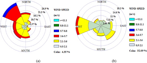
The average of the azimuths of the 2 stations in the studied months was 292.5°.

Wind shelter index (Sx)

The dominant wind direction in the region had an azimuth of 292.5° in the center of the sector, which was located between the azimuths of 262.5° and 322.5° (Figure 5). At each point in the grid, a sector with 13 directions was considered, with each direction including 101 points with steps of 50 m, so that the direction of the prevailing wind of the region passed through the center of this sector.

Figure 5. Impact bounds of wind direction with azimuth 262.5 to 322.5º (13 directions), for one of the grid points.

Determining the effective length

The difference between the successive values of Sx reached its maximum at the 2 lengths of 1000 and 500 m (Figure 6). That is, Sx values for a length of 1000 m had the highest value compared to other indexes at other lengths. Therefore, 1000 m was selected as the effective length of the study area, and the corresponding wind shelter values were introduced as Sx values for the points.

Figure 6. The average of differences of Sx in each consecutive 2 lengths for (a) Jun, (b) Jul, (c) Aug, and (d) Sep.

Validation and sensitivity

Of the 4 months, September had the lowest average water level (Table 1). The average water level decreased from June to September, while the average Sx increased. The Sx values at the points located near the surrounding topography (along the lake’s margin) were on average 94.3% higher than the points farther away from the elevations (at the central parts of the lake; Table 1).

Table 1. Average values of water level and wind shelter index.

Month	Average water level (m)	Average Sx (degrees)	Average Sx value for points located on the lake margin (degrees)	Average Sx value for points located in the central parts of the lake (degrees)
Jun	345.5	0.050	0.123	0.007
Jul	343.5	0.053	0.129	0.007
Aug	338	0.059	0.141	0.008
Sep	331	0.071	0.168	0.010

Since the western mountains of the lake were taller than 870 m (Figure 1) and the prevailing wind direction of the region was from the northwest (Figure 5), it is perhaps not surprising that parts of the lake located on the western margin of the lake have larger Sx values (Table 1, Figure 3). This confirms the calculation of the Sx.

Examination of the relationship between Sx values and surface water level changes (Table 1) showed that Sx variations were sensitive to the lake water level changes, such that from June to September, on average, a 14.5 m decrease in water level caused a 47.16% (0.021°) increase in Sx value. Also, examining Sx variations with water level changes showed that a 13.79% decrease in the water level between June and July corresponded with a 20.42% increase in Sx value (Table 2). In August and September, 34.48% and 51.72% reductions in water level compared to the preceding months coincided with Sx values increased by 47.56% and 73.5%, respectively.

Table 2. Percent reduction in water surface height and increase in wind index in each month compared to the previous month.

Variables	Jul vs. Jun	Aug vs. Jul	Sep vs. Aug
Water level decrease (%)	13.79	34.48	51.72
Average Sx increase (%)	20.42	47.56	73.5

A 50% reduction of the reservoir water level, caused by both the type of reservoir operation and the climatic conditions of the region during the 4 months of the warm season, increased the value of Sx (0.021°; Table 1). Dez Dam is one of the most important dams in Iran and its water storage is used for agriculture, drinking, and hydropower generation. Since it does not rain in the warm months of the year in most parts of Iran, water consumption increases during these months. Therefore, high release, on the one hand, and no rain and supply to the reservoir in these months, on the other hand, cause a decrease in the water level of the reservoir and, as a result, an increase in the Sx.

Sx cluster analysis

An initial comparison of the Ward and K-means methods showed that there was not much difference between the 2 methods. For example, in the Ward method, on average, 66.1% of the lake area with an average Sx of 0.016° was less exposed to wind shelter than other areas of the lake. In addition, 18.7%, 9.3%, 4.7%, and 1.3% of the basin area were placed in clusters 2, 3, 4, and 5, with an average Sx of 0.093°, 0.236°, 0.453°, and 0.765°, respectively (Table 3). Also, in the K-means method, the average areas allocated to 5 clusters were 78.6%, 14%, 5.1%, 2.1%, and 0.16%, with an average Sx of 0.014°, 0.136°, 0.314°,0.519°, and 0.795°, respectively. However, comparing the clustering results of the 2 methods with the Sx raster maps (Figure 3) showed that the Ward method had a better fit. In the K-means method, many points around the island in the middle of the Dez Dam lake (Figure 7(a)) were assigned to cluster 5, while a review of the Sx raster maps (Figure 3) showed that the wind sheltering at most of these points was only slightly higher than in the central parts of the lake. That is, the K-means method allocated a large area to cluster 5 than the actual area. Due to the large amount of data generated by both methods, only the Ward method results are presented (Table 3, Figure 7).

Figure 7. Clustered area of Lake Dez dam on the basis of cluster analysis of Sx using Ward method in (a) Jun, (b) Jul, (c) Aug, and (d) Sep.

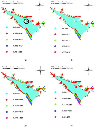
Table 3. Clustering statistical parameters using the Ward method.

Month	Factors	Cluster 1	Cluster 2	Cluster 3	Cluster 4	Cluster 5
Jun	Sx variations (%) in each cluster	0–0.049	0.049–0.127	0.127–0.319	0.32–0.535	0.537–1.109
	Area of each cluster vs. total area of the lake (%)	75.6	12.8	8.2	3.0	0.4
	Average Sx in each cluster (degrees)	0.009	0.081	0.2	0.407	0.682
Jul	Sx variations (%) in each cluster	0–0.039	0.039–0.163	0.163–0.411	0.412–0.737	0.74–1.118
	Area of each cluster vs. total area of the lake (%)	70.8	19.2	7.8	2.2	0.01
	Average Sx in each cluster (degrees)	0.039	0.163	0.411	0.737	1.118
Aug	Sx variations (%) in each cluster	0–0.03	0.03–0.116	0.117–0.216	0.216–0.399	0.4–1.133
	Area of each cluster vs. total area of the lake (%)	62.3	21	8.02	5.5	3.2
	Average Sx in each cluster (degrees)	0.006	0.063	0.159	0.292	0.55
Sep	Sx variations (%) in each cluster	0–0.034	0.034–0.115	0.115–0.256	0.257–0.571	0.573–1.155
	Area of each cluster vs. total area of the lake (%)	55.5	21.9	13.2	8.1	1.4
	Average Sx in each cluster (degrees)	0.008	0.066	0.174	0.376	0.709
Average area of each cluster vs. total area of the lake (%)		66.1	18.7	9.3	4.7	1.3
Average Sx in each cluster during the studied period (degrees)		0.016	0.093	0.236	0.453	0.765

By differentiating areas of the lake based on wind sheltering, we identified which areas were most exposed to evaporation and thus should be considered priority areas for implementing evaporation control projects. Accordingly, the points located in cluster 1, with an average Sx of 0.016° (Table 3), which accounted for 66.1% of the lake area, were more suitable than other areas with higher Sx for performing evaporation reduction methods.

Implications for management

In mountainous regions, the surfaces of open water reservoirs, including dam reservoirs such as the Dez Dam reservoir, are exposed to varying degrees of wind due to the surrounding topography. Given that the rate of evaporation and consequently the amount of evaporation is higher in areas exposed to the wind than in the sheltered areas, the evaporation rate varies due to wind in different parts of the lake. Based on the methodology used in this study, it is possible to evaluate open water reservoir surfaces to determine wind shelter conditions in different clusters of the surface, information that can then be applied to reducing evaporation at the surface of reservoirs. In this study, we were only able to predict which locations are most exposed to evaporation. Therefore, the development of a mathematical model regarding the value of the Sx and rate of evaporation, as well as the point or polygon velocity of the wind, can complement the idea of a wind shelter index (Sx). Accordingly, the surface of Dez Dam lake was classified based on the relative evaporation intensity in the form of 5 clusters.

Acknowledgments

This study was conducted using data provided by the Ahvaz Meteorological Organization and Ahvaz Cartographic Center. We warmly thank these 2 organizations. Also, we are grateful to the Research Council of the Shahid Chamran University of Ahvaz for financial support (grant number SCU.WH98.26878).

References

- Barnes GT. 2008. The potential for monolayers to reduce the evaporation of water form large water storage. J Agric Water Manage. 95(4):339–353. doi:10.1016/j.agwat.2007.12.003.
- Berg NH. 1986. Blowing snow at a Colorado alpine site: measurements and implications. J Arct Alp Res. 18(2):147–161. doi:10.2307/1551124.
- Choi YK. 2014. A study on power generation analysis of floating PV system considering environmental impact. IJSEIA. 8(1):75–84. doi:10.14257/ijseia.2014.8.1.07.
- Cluff CB. 1977. Evaporation control for increasing water supplies. For Presentation at Conference on Alternative Strategies for Desert Development and Management, Sacramento, California, May 31–June 10; p. 1–14.
- Craig IP. 2005. Loss of storage water due to evaporation-a literature review. NCEA Publication. University of Southern Queensland. Australia. https://core.ac.uk/download/pdf/11036429.pdf.
- Craig IP, Aravinthan V, Baillie CP, Beswick A, et al. 2007. Evaporation, seepage and water quality management in storage dams: a review of research methods. J Environ Health. 7(3):84–97.
- Craig IP, Green A, Cobie M, Schmidt E. 2005. Controlling evaporation loss from water storages: Rural water use efficiency initiative. NCEA Publication No: 1000580/1. National Centre for Eng in Agric University of Southern Queensland. Depart of Natural Resour and Mines. Queensland, Toowoomba.
- Dozier J, Bruno J, Downey P. 1981. A faster solution to the horizon problem. J Comput Geosci. 7(2):145–151. doi:10.1016/0098-3004(81)90026-1.
- Elder K. 1995. Snow distribution in Alpine watersheds [dissertation]. Santa Barbara (UC): University of California.
- Erickson TA, Williams MW, Winstral A. 2005. Persistence of topographic controls on the spatial distribution of snow in rugged mountain. J Water Resour Res. 41(4):1–17. doi:10.1029/2003WR002973..
- Farokhzadeh S, Sharifi MR, Moradi S, Akhond Ali AM. 2014. Wind shelter index’s effective distance determination in non-snowy watershed basins. J Adv in Environ Biol. 8(5):1431–1441.
- Gokbulak F, Ozhan S. 2006. Water loss through evaporation from water surfaces of lake and reservoirs in Turkey. Official Publication of the European Water Association (EWA). Turkey. https://www.ewa-online.eu/tl_files/_media/content/documents_pdf/Publications/E-WAter/documents/40_2006_07.pdf.
- Gong X, Richman MB. 1995. On the application of cluster analysis to growing season precipitation data in North America East of the rockies. J Climate. 8(4):897–931. doi:10.1175/1520-0442(1995)008 < 0897:OTAOCA>2.0.CO;2..
- Habibi A. 2015. SPSS Applied Training. Iran (Ir): Fourth edition. p. 135–139. Persian.
- Jennison I. 2003. Methods for reducing evaporation from storages used for urban water supplies. Final Report. Dep of Nat Resour and Mines, Queensland, Australia.
- Litaor MI, Williams M, Seastedt TR. 2008. Topographic controls on snow distribution, soil moisture, and species diversity of herbaceous alpine vegetation, Niwot Ridge, Colorado. J Geophys Res 113:1–10. 10.1029/2007JG000419.
- Maroufi S, Tabari H, Zare Abiane H, Sharifi M. 2010. Investigation of wind effects on spatial distribution of snow accumulation in one of Karoon sub-basins (case study-Samsami basin). J Geophys Res. 1(2):31–44. Persian.
- Molotch NP, Bales RC. 2006. SNOTEL representativeness in the Rio Grande headwaters on the basis of physiographic and remotely sensed snow cover persistence. Hydrol Process. 20(4):723–739. doi:10.1002/hyp.6128.
- Molotch NP, Colee MT, Bales RC, Dozier J. 2005. Estimating the spatial distribution of snow water equivalent in an alpine basin using binary regression tree models: the impact of digital elevation and independent variable selection. Hydrol Process. 19(7):1459–1479. doi:10.1002/hyp.5586.
- Sarang A. 2001. Reporting the status of water resources of Iran: Challenges and solutions. Water and Environ Res Center of Sharif University of Technology, Tehran, Iran. Persian. http://ewrc.sharif.edu.
- Sharifi MR. 2007. Investigation of the spatial distribution of snow equivalent water using combined methods [dissertation]. Shahid Chamran University of Ahvaz. Persian.
- Sharifi MR, Akhond Ali AM, Porhemmat J, Mohammadi J. 2007. Evaluation of two methods of linear correlation equation and the ordinary kriging in order to estimate the spatial distribution of snow depth in Samsami watershed basin. J Iran-Watershed Manage Sci Eng Res 1(1):24–38. Persian. http://jwmsei.ir/article-1-25-fa.html.
- Tabari H, Marofi S, Zare Abyaneh H, Sharifi MR. 2010. Comparison of artificial neural network and combined models in estimating spatial distribution of snow depth and snow water equivalent in Samsami basin of Iran. Neural Comput Appl. 19(4):625–635. Persian. doi:10.1002/hyp.6128..
- Vara-Orta F. 2008. A reservoir goes undercover. Los Angeles Times. http://articles.latimes.com/2008/jun/10/local/me-balls10.
- Winstral A, Elder K, Davis RE. 2002. Spatial snow modeling of wind-redistributed snow using terrain based parameters. J Hydrometeor. 3(5):524–538. doi:10.1175/1525-7541(2002)003 < 0524:SSMOWR>2.0.CO;2..
- Winstral A, Mark D, Gurney R. 2009. An efficient method for distributing wind speeds over heterogeneous terrain. Hydrol Process. 23(17):2526–2535. doi:10.1002/hyp.7141.