Hydrology of annual winter water level drawdown regimes in recreational lakes of Massachusetts, United States

Abstract

Carmignani JR, Roy AH, Stolarski JT, Richards T. 2021. Hydrology of annual winter water level drawdown regimes in recreational lakes of Massachusetts, United States. Lake Reserv Manage. 37:339–359.

Annual winter water level drawdown (WD) is a common lake management strategy to maintain recreational value by controlling nuisance macrophytes and preventing ice damage to shoreline infrastructure in lakes of the northeastern United States. The state of Massachusetts provides general guidelines for lake managers to implement and practice WDs. However, WD management reporting is not required and as such empirical water level records are scarce, making it difficult to assess guideline adherence and link these management actions to littoral habitat conditions. We monitored water levels bihourly in 18 lakes with ongoing WD regimes and 3 non-drawdown lakes over 3–4 yr. Our results show an interlake drawdown magnitude gradient of 0.07–2.66 m with intralake consistency across years. Corresponding WD magnitudes generated exposure of 1.3–37.6% for entire lakebeds and 9.2–71.1% for littoral zones. WD durations averaged 171 d and ranged widely from 5 to 246 d. Longer recession and refill phase durations and faster recession rates were moderately to strongly correlated with drawdown magnitudes. WDs were predominantly initiated prior to the state of Massachusetts 1 November starting guideline (83.1%) and refilled to summer reference levels after the recommended date of 1 April (70.6%). To minimize ecological impacts while still meeting recreational goals, WD performance guidelines may require a more fine-scale approach that integrates local hydrogeomorphic features and the presence of WD-sensitive littoral biotic assemblages. However, climate change model projections of warmer and wetter winters in the Northeast indicate increasing uncertainty for WD as an effective and worthwhile macrophyte control tool.

Keywords:

• Benthic exposure
• drainage ratio
• drawdown magnitude
• macrophyte management
• recession rate
• refill timing

Lake water level fluctuations compose a natural hydrological regime whose intra- and interannual variability in magnitude, timing, rate, frequency, and duration of high and low water level events influence biogeochemical patterns and processes in littoral zones of natural lakes (Wantzen et al. 2008a). Water level fluctuation regimes in lakes with outflow control structures can significantly deviate from water level regimes in natural lakes (Kennedy 2005). Consequently, changes to the magnitude, timing, duration, rate, and frequency of high and low water level events can alter and degrade lake and littoral zone ecological conditions (Wantzen et al. 2008b, Miranda et al. 2010, Zohary and Ostrovsky 2011). The direction and strength of various ecological responses to altered lake water levels depend on the specific hydrologic metrics and resident biota (Hill et al. 1998, Eloranta et al. 2018). Therefore, reliable prediction of ecological responses and mitigation of negative impacts to littoral zone communities require accurate quantification of regulated water level fluctuations.

Annual winter water level drawdowns (WDs) are an example of a regulated water level regime that is regularly performed in temperate and boreal lakes as a consequence of wintertime power demand in hydroelectric lakes or to provide spring flood storage (Hellsten 1997). In recreational lakes of Massachusetts and other states in the northeastern United States, WDs are used to improve recreational value (e.g., boating, swimming) by attempting to reduce nuisance densities of macrophytes and protecting shoreline structures (e.g., docks, retaining walls) from ice damage (Mattson et al. 2004). Water levels in WD regimes are lowered in autumn, reach target drawdown levels in winter, and are refilled in the spring (e.g., Mjelde et al. 2013, Carmignani and Roy 2017). Previous studies, primarily from hydroelectric and storage lakes in Scandinavia and Canada, have characterized WD hydrology to explain patterns in littoral zone communities predominantly as a function of WD amplitude and referred to hereafter as magnitude (e.g., White et al. 2011, Mjelde et al. 2013). For example, Sutela et al. (2013) quantified WD magnitude as the 20 yr mean difference between the highest and lowest water level per winter in 16 regulated lakes in Finland. Ecological quality indices, represented by macrophytes, macroinvertebrates, and fish littoral assemblages, decreased with drawdown magnitude.

In contrast to hydroelectric lakes, the spatiotemporal variability of WD regimes in northeastern US recreational lakes has not been quantified despite its widespread and historical prevalence. Due to differences in climate, watershed and lake hydromorphological features, and water level management goals, WD regimes in recreational lakes in the northeastern United States likely differ compared to hydroelectric lakes in north temperate and boreal zones. Consequently, ecological responses to WDs in recreational lakes may differ, requiring quantification of water level fluctuation to reliably estimate potential ecological impacts (e.g., Carmignani et al. 2019). Furthermore, while most studies focus on WD magnitude, other hydrological components, such as timing, duration, water level recession and refill rates, and degree and duration of lakebed exposure, may help to better predict ecological responses (Carmignani and Roy 2017, Hirsch et al. 2017). For example, the timing of low spring water levels contributes to low recruitment of spring spawning fish species that reproduce in shallow depths of the littoral zone (Linløkken and Sandlund 2016).

We aimed to better understand the hydrology of annual winter drawdowns in recreational lakes in Massachusetts, through continuous water level monitoring of WD lakes over several years. Our objectives were to (1) assess the interlake and interannual variability of WD timing, magnitude, rate, and duration, and (2) evaluate the correspondence of empirical WD metrics with the magnitude, timing, and recession rate performance standards issued by the Massachusetts Division of Fisheries and Wildlife for WD events (MassWildlife 2002) and restated in the Massachusetts Generic Environmental Impact Report on Eutrophication and Aquatic Plant Management (Mattson et al. 2004). Mattson et al. (2004) provide general guidance to implement and perform WDs in Massachusetts to minimize impacts to in-lake and downstream nontarget organisms (e.g., mollusks, amphibians, reptiles, spawning fish species, mammals) and water-supply availability in local wells, while managing macrophytes. Hydrologic data collected in this study can provide insight on how WDs are performed in Massachusetts and guide future WD management in northeastern US recreational lakes to help balance ecological sustainability and recreational value, and to help guide realistic WD implementation in the face of climate change.

Study site

We selected 18 lakes in western and central Massachusetts with current WD regimes and 3 lakes with no history of annual winter drawdowns (Figure 1, Table 1) using a stratified random approach to primarily capture a WD magnitude gradient (see Methods S1 in the Supplement for full details). Briefly, we stratified a set of 271 lakes of area ≥ 0.035 km² with historical WD information by lake area, lakeshore residential development within a 100 m riparian buffer, and reported WD magnitude information, creating several group combinations from natural breaks in data distributions. We also targeted lakes in all level IV US Environmental Protection Agency (USEPA)-defined ecoregions within the level III Northeastern Highlands and 2 level IV ecoregions in the level III Northeastern Coastal Zone to help reduce water quality variation among waterbodies based on watershed land cover and geology for a related study effort on macrophytes (Methods S1). From stratification groups we randomly selected 16 WD lakes and 4 non-drawdown lakes. We were unable to access 4 WD and one non-drawdown lakes and therefore replaced them with 6 additional WD lakes within the study ecoregions and within the range of stratification criteria.

Figure 1. Map of study lake locations within the state of Massachusetts. Circles represent lakes with annual winter drawdown water level regimes (WD) and triangles represent lakes with no history of WDs. USEPA boundaries are level III ecoregions.

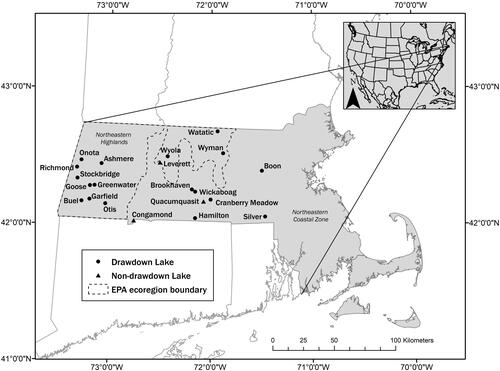
Table 1. Morphometric features and winter drawdown history of study lakes. Non-WD = non-winter drawdown lake, WD = winter drawdown lake, WL = water levels, NK = data not known, TP = total phosphorous. Drainage ratio = watershed:lake area.

Lake	Years WL monitored	WD status	Decade WD implemented	Lake (km^2)	Drainage ratio	Mean/maximum depth (m)
Leverett	4	Non-WD	–	0.39	4.4	1.7/6.5
Quacumquasit	4	Non-WD	–	0.94	5	7.6/25.7
Congamond	3	Non-WD	–	1.93	4.4	5.6/14.1
Silver	4	WD	2000s	0.19	22.6	1.5/2.8
Buel	3	WD	2010s	0.83	17.1	5.1/14.4
Brookhaven	4	WD	1970s	0.14	25.7	1.5/3.8
Boon	4	WD	2000s	0.73	7.0	2.8/7.7
Watatic	4	WD	NK	0.56	28.0	2.0/4.6
Cranberry Meadow	4	WD	NK	0.30	6.3	1.5/3.0
Wyman	4	WD	1990s	0.87	22.6	1.6/5.4
Greenwater	4	WD	1950s	0.38	10.3	5.0/18.6
Wickaboag	3	WD	1960s	1.30	34.5	1.9/3.8
Richmond	4	WD	1960s	0.95	21.5	2.9/17.2
Wyola	3	WD	1970s	0.50	35.2	3.4/10.1
Hamilton	3	WD	1990s	1.68	27.7	1.8/6.4
Ashmere	4	WD	1950s	1.14	10.1	3.4/8.3
Stockbridge	4	WD	1980s	1.60	18.6	5.4/15.9
Onota	4	WD	1970s	2.66	10.3	4.1/24.7
Goose	4	WD	1920s	1.30	8.5	5.0/16.3
Garfield	3	WD	1970s	1.11	9.3	3.8/10.8
Otis	5	WD	1960s	4.21	9.9	4.5/17.4

All study lakes possess an outflow control structure and can be defined as natural drainage lakes (n = 14) or impounded lakes (n = 7; Whittier et al. 2002). We define natural drainage lakes as lentic systems that had an original state of >10 ha before lake area enhancement via mill operations, water supply, and/or flood storage, among other reasons. We define impounded lakes as dammed stream systems constructed for similar reasons. These lake types are common in Massachusetts and are also representative of the 2 most prevalent lakes types in the Northeast region (Whittier et al. 2002). Hereafter, both waterbody types are referred to as lakes. Most lakes are outfitted with a valve or gate (n = 14) to control lake water levels and outflows, while a minority use wooden stopboards (n = 7).

Inland Massachusetts has a continental temperate climate with 4 seasons. Mean minimum/maximum July and January temperatures for western Massachusetts tend to be 1–3 C lower than in central Massachusetts (Griffith et al. 2009), and winter precipitation averages 21.6–25.4 cm (1981–2010) across these general regions (https://www.ncdc.noaa.gov/cdo-web/datatools/normals). Lake ice-on typically occurs from December to January and ice-off between February and early May in Massachusetts lakes (Hodgkins et al. 2002). Stream inflows generally are highest in spring months (Mar–May), decline throughout the summer (Jun–Sep), increase in the fall (Oct–Nov), and decline again through the winter (Huntington et al. 2009). Watersheds of study lakes have mixed land use with variable urban development ranging from 2 to 40% (median = 9%) with a general increase from west to east, and relatively small proportions of pasture (0–15%) and agriculture (0–8%). Concomitantly, total watershed forest cover ranges from 20 to 83% (median = 64%) among lakes (MRLC 2018). Forests are primarily composed of mixed deciduous and conifer stands, including northern, central, and transition hardwoods (Griffith et al. 2009). Watersheds are underlaid by various geologies across the study area. Lakes located in the Northeast Highlands are characterized by coarse-loamy to loamy soils and metamorphic bedrock- or limestone-derived coarse-loamy soils and calcareous bedrock (Griffith et al. 2009). In central Massachusetts or the Northeast Coastal Zone, lakes are underlain with sedimentary bedrock and alluvium soils, metamorphic bedrock with coarse-loamy soils, or coarse-loamy and sandy soils (Griffith et al. 2009).

Materials and methods

Water level monitoring and quality control

Water levels were monitored continuously from fall 2014 to fall 2018 at 18 drawdown and 3 non-drawdown lakes. We deployed paired nonvented pressure transducers (Onset HOBO U20L-01, Bourne, MA) in 14 lakes in September–October 2014 and in 6 lakes in September–November 2015 to collect pressure and temperature at bihourly intervals (Table 1). Water level data for Otis were provided by the Massachusetts Department of Conservation and Recreation, where data started in March 2012 up to May 2018. Water level data collection ceased in May–November 2018, resulting in 2–4 yr of winter water levels per lake (6 for Otis). We generally followed methods from Stamp et al. (2014) for pressure transducer (i.e., logger) installation and monitoring. In each lake we installed paired loggers adjacent to the point of lake outflow, one underwater and one above water on shore. If access was limited, we installed underwater loggers adjacent to access points (e.g., bridges, culverts) in other parts of the lake. All loggers were sheltered in PVC housing. Underwater loggers were fixed to dam or bridge abutments and suspended on nonstretch cable within a PVC pipe. If we could not attach an underwater logger to a fixed structure, loggers were fixed to a wood stake or metal pipe that was anchored into the lakebed. All loggers were set to record at 2 h intervals. We downloaded data from loggers at least twice per year, pre- and post-drawdown event, and recorded relative elevation from a secondary fixed location (e.g., staff gauge, spillway, dam abutment) to help identify unintentional logger movement from ice formation/melt and instrument accuracy drift.

Paired pressure measurements were converted to water levels using HOBOWarePro software (version 3.7.8, Onset Computer Corporation, Bourne, MA) and imported into R software. We used the ContDataQC package (Leppo et al. 2017, version 2.0.2.9001) in R (R Core Team 2017, version 3.4.2) to identify potential inaccurate water level records based on water level change and minimum and maximum records. We flagged records with an absolute change of ≥3 cm and adjusted preceding data to account for apparent transducer movement or drift derived from discrete water elevation measurements from secondary locations. We removed negative water level records and values <1 cm that are unreliable measurements. Additionally, we examined water temperature data coupled with pressure measurements to help identify inaccurate water level records, such that records with water temperatures <0 C were flagged for inspection. To compensate for lost barometric air pressure readings at Wyola (19 Jun 2017–2 Nov 2018) and hence estimate water levels, we used predicted air pressure records generated from the closest study lake at Leverett (7.2 km from Wyola).

Water level metrics

We defined 2 general water level time periods to calculate water level metrics: the WD period or event and the summer or the non-drawdown period. We further split the WD period into 3 time frames or phases: water level decline (recession phase), drawndown water levels (stable phase), and the period of refill to predefined normal pool levels (refill phase, Figure 2). We first isolated WD periods by visually identifying the recession initiation date as the first record of consistent water level decline in the fall and the refill phase end date as the first record of increasing water levels that culminate in predefined summer pool levels in winter–spring. Summer or normal pool water levels were defined as the median water level from non-drawdown periods in 2015 (n = 15) or from spillway elevations (n = 6). Within the WD period, the end of water level recession or the start of the stable phase was marked by no consistent water level increase or decrease. The start of the refill phase was marked by a consistent visual water level increase in the hydrograph with no clear water level decline before reaching reference water levels. These water level phase boundaries were visually inspected over a 14 d period. These definitions allowed for the inclusion of precipitation or melting events to influence recession and refill phases. For non-drawdown lakes, we divided water level records into spring/summer and fall/winter period that covered 2 April–30 September and 1 October–1 April, respectively, to generally correspond to summer and WD periods in drawdown lakes. For the summer period and each of the WD period phases (e.g., recession, stable, refill), we calculated basic summary statistics including duration, minimum, maximum, medians, and selected quantiles.

Figure 2. (A) Example hydrograph and associated winter drawdown (WD) metrics calculated for a single WD period. Water levels (y axis) are relativized to reference water level (e.g., summer/normal pool level) such that relative water level = 0 represents normal pool level. WD period phases (in italics and gray shades) include the recession, stable, and refill phases. Vertical dotted lines and changes in background color indicate the start and end dates for WD phases. These dates are used to calculate WD duration, recession and refill rates, and WD magnitude. Duration exposed for a given depth (e.g., 0.5 m, 1 m) corresponds to elapsed time when relative waters exceeded this depth. (B) Example of recession and refill rates through time for a WD period, with boxplot displaying interquartile range and extreme values >1.5 times the interquartile range; this can be inferred from plot. (C) Photos corresponding to changes in water level throughout a WD period as labeled in (A).

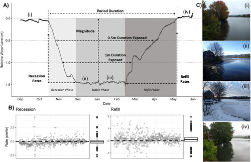
For each WD event, we quantified magnitude, recession and refill rates, and WD duration, and identified the timing of each WD phase (Figure 2). We calculated magnitude as the difference between reference pool level and the (1) maximum (i.e., lowest) water level recorded during the entire WD period, and (2) mean water level during the stable phase. Rates of recession and refill were calculated using consecutive records and summarized into median, minimum, and maximum values, and scaled from cm/h to cm/d for ease of interpretation. Durations were determined in days for the entire WD period (i.e., recession start to refill end) and for each stable phase. Further, we calculated duration of exposure/emersion at 0.25 m depth intervals from 0.25 to 2.0 m depth contours relative to reference water levels. These WD metrics were calculated using bihourly records except for daily water level data at Otis between October 2015 and May 2018. Results are reported using median WD metric values and ranges per WD event.

Bathymetry collection and analysis

We sampled depths for all lakes in April–June 2015 or 2016 when water levels were at or above normal pool levels. Following a cross-hatched pattern over the lake surface, depths were measured using a Garmin GPSMAP 431s with 1309–48,803 sample points per lake, depending on surface area. We used empirical Bayesian kriging in ArcGIS 10.3 to interpolate unsampled depths from empirical depths (Krivoruchko 2012; see Methods S2 in the Supplement for details).

We estimated the maximum depth of macrophyte colonization as a surrogate of littoral zone boundaries to determine the lakewide littoral zone area modified from Perlelberg et al. (2016). We established 4 to 21 transects scaled by lake area <10 m in depth to sample macrophyte presence from 29 August to 9 September 2017. Transects were equally spaced along the 10 m depth contour or deepest depth contour within a lake or distinct lake basins. We sampled macrophytes along transects perpendicular to depth contours at 0.5 m depth intervals using a double-headed rake suspended by rope. The rake was dragged approximately 0.5–1 m along the bottom at each sampling point and was then inspected for macrophyte or macroalgae presence. Maximum depth values per transect were averaged for each lake and incorporated into littoral area exposure calculations for given WD events. If macrophytes were sampled at the deepest point of a lake, we assumed the littoral zone was equivalent to the entire benthic area.

Calculation of lakebed and littoral zone exposure required coupling interpolated depths with water level records and applying WD magnitudes to bathymetry data. First, depths were matched to contemporaneous water level records at the time of bathymetry surveys. Then we found the simple difference between reference water levels and water levels at matching times. If the difference in water levels was greater than the accuracy of the pressure transducers (1 cm), we applied the difference to magnitudes to estimate exposure area metrics more accurately. We calculated area of lakebed and littoral area exposure as the number of 1 m² depth cells for lake and littoral areas less than the maximum magnitude for a given WD event. Areas exposed were expressed as percentage of the whole lake and littoral areas to compare across lakes.

We also determined ratios of watershed to lake area (drainage ratios) to potentially explain WD water level metric variability. To calculate watershed areas, we delineated watersheds from the point of lake outflow using spatial analyst tools in ArcGIS 10.3 (ESRI 2015) based on the 3 m US Geological Survey Digital Elevation Model. Finally, we calculated Spearman rank correlation coefficients among WD medians of period and phase durations, magnitude, exposures, rates, and drainage ratios.

Comparison to state guidelines

We compared observed water levels to the magnitude, timing, and recession rate guidelines of MassWildlife (2002) and Mattson et al. (2004). These performance standards were developed to protect in-lake and downstream ecological integrity using the best scientific evidence at the time while still meeting the proposed goals of WD, namely, macrophyte control. The guidelines recommend magnitudes <3 feet (i.e., 0.914 m), for recessions to start after 1 November, reach target stable phase water levels by 1 December, and to refill to normal lake levels by 1 April, and for recession rates to not exceed 3 inches/d (i.e., 7.62 cm/d). Initiating WDs after 1 November prevents reductions in already low dissolved oxygen levels within shallow vegetated basins and flushing this water downstream, which can cause in-lake and downstream fish kills. Meeting target stable phase water levels by 1 December enables hibernating biota (e.g., amphibians, reptiles, beavers, muskrats) to relocate before substrate freezing and lake ice-on. Refilling to normal pool level by 1 April will ensure limited impact to available fish spawning habitat of spring littoral spawning species (e.g., chain pickerel, Esox niger; yellow perch, Perca flavascens). Lastly, recession rates are capped to maintain natural flows downstream and prevent stranding of fish and other aquatic organisms. If lake managers aim to deviate from the WD performance standards, municipal conservation commissions in coordination with state agencies can permit special WD performance conditions to meet management goals of macrophyte control. Several lakes are permitted to initiate WDs by 1 October (Boon), 15 October (Goose, Otis, Wickaboag, Watatic), or sometime after Columbus Day (i.e., the second Monday in October; Hamilton) before the 1 November state recommendation. Additionally, several lakes are permitted to perform WDs with magnitudes >0.914 m (Otis, Goose, Onota, Garfield). Although several lakes possess special WD performance conditions that differentiate from state guidelines, we do not assess whether these lake-specific permit conditions were met. Rather, we highlight these special cases within the results when comparing against the original MassWildlife (2002) guidelines.

For WD magnitudes we identified the number and proportion of WD events of >0.914 m. For timing, we identified the percentage of WD phases that did and did not meet corresponding phase timing guidelines. For recession rates, we calculated net water level rates over a 24 h moving window to compare against the recommended ≤3 inches/d (i.e., 7.62 cm/d) of water level decline. We determined the percentage of net daily recession rates ≥7.62 cm/d for each recession phase and determined the number of recession events for which the median recession rate was ≥7.62 cm/d of water level decline.

Results

We captured 2–4 complete WD events per WD lake and 3–4 yr of water level data for non-drawdown lakes. Overall, we collected water level data on 69 complete WD events across 18 lakes. Due to the timing of logger installation and logger failure, we did not capture complete recession phase durations in 2014–2015 for Brookhaven and Silver, in 2015–2016 for Hamilton, Wickaboag, and Wyola, and stable and refill phases at Cranberry Meadow in 2015–2016.

Drawdown versus non-drawdown lakes

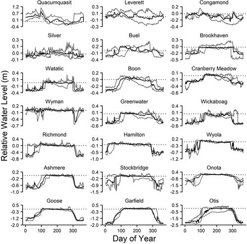
Overall, hydrology of WD lakes differed from that of non-drawdown lakes, particularly during winter months (Figure 3). In non-drawdown lakes, median water levels in winter months (i.e., 1 Oct–1 Apr) ranged from 13.2 cm below reference pool level to 62.4 cm above reference pool level. The lowest winter water levels ranged from 5.7 to 31.6 cm below reference pool levels, with the extreme lowest water levels occurring in the 2016–2017 winter across all non-drawdown lakes. In comparison, median water levels in WD lakes across WD periods ranged from −202.4 to 0.1 cm. Median summer water levels varied across years, with the lowest water levels in 2016, but were similar across WD and non-drawdown (WD: median = 0.1 cm, range = −58.9 to 45.6 cm; non-drawdown: median = 0.5 cm, range = −30.0 to 102.4 cm).

Figure 3. Water level time series for study lakes. Water levels are expressed relative to reference pool level (relative water level = 0, dotted line). Black lines indicate water level medians, and gray lines represent the range per day of year over 3–4 yr. Note that y-axis scale varies by lake. See Figure 1 for lake locations.

Magnitude

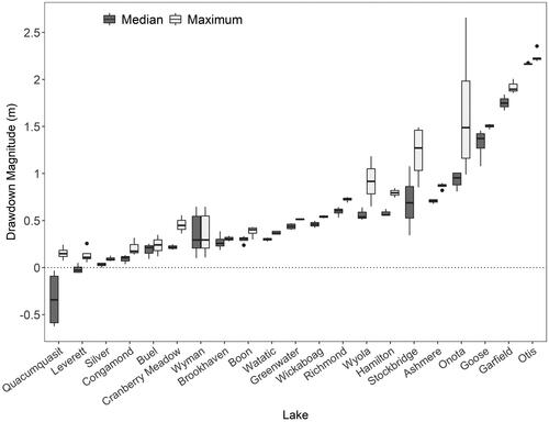
We captured a magnitude gradient with interannual median of stable phase water levels ranging from 0.001 to 2.16 m with an overall median of 0.66 m across lakes (Figure 4, Table S1). Median maximum magnitudes (i.e., lowest water levels below reference levels) ranged from 0.09 to 2.23 m with a lowest maximum magnitude of 0.07 m at Silver and the highest at 2.66 m at Onota (Figure 3). Median water levels during stable phases were consistent among years for most lakes, varying <10 cm for 9 lakes and <20 cm for 14 lakes. Onota showed the highest interannual variability in maximum magnitude (1.67 m) because of a regime with a sequence of 2 shallow drawdowns and one deep drawdown in successive years. Maximum magnitudes exceeded the 0.914 m magnitude guideline recommended by MassWildlife (2002) in 6 of 18 WD lakes and 20 of 74 WD periods (27%) consistently (e.g., Otis, Onota, Garfield, Goose) or variably (e.g., Stockbridge 3 of 4, Wyola 1 of 3) among years. Median stable phase water levels for 5 lakes also variably exceeded this threshold among years (e.g., Otis, Onota, Garfield, Goose, Stockbridge). Four of these lakes (Otis, Onota, Garfield, Goose) were permitted to exceed the magnitude guideline.

Figure 4. Interannual magnitudes categorized as median (dark gray bars) and maximum (light gray bars) water levels during the stable phase. Non-drawdown lakes are Quacumquasit, Leverett, and Congamond.

Area exposed

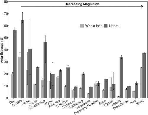
Interannual median lake exposure ranged from 1.3% to 34.2% across lakes (Figure 5, Table S2). Median littoral exposure ranged from 9.3% to 64.8% across lakes (Figure 5). Lake area and littoral area exposed was largely within 10% exposure difference among years for most lakes, except for Onota, Stockbridge, Wyola, and Wyman. Onota displayed the highest interannual variability in lake and littoral percent exposure. The highest maximum magnitudes typically equated to the highest littoral and lake area exposed. However, relatively small magnitudes at a few lakes resulted in relatively high percent littoral and lake area exposed (e.g., Silver, Watatic). Conversely, several lakes with moderate to high magnitude had relatively low percent exposures (e.g., Goose).

Figure 5. Median (± range) percent lake area and littoral area exposed at maximum drawdown magnitudes. Lakes are ordered by decreasing mean drawdown magnitude.

Durations

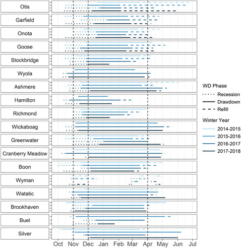
WD period durations ranged from 5 to 246 d with an overall median of 171 d (Figure 6, Table S2). Otis exhibited the longest median duration at 236 d and Wyman the shortest at 17 d. WD duration varied interannually within lakes from 24 to 175 d with a median of 54 d. The recession phase comprised 19.4%, the stable phase 62.5%, and the refill phase 13.5% for a median WD period. WD phases also exhibited wide variability. The recession phase varied from 3 to 70 d (median = 24 d), the stable phase from 0 to 215 d (median = 98 d), and the refill phase from 0 to 139 d (median = 17 d, Table S2).

Figure 6. WD period duration and timing for 3 or 4 drawdowns per lake (color coded by year). Each WD period is divided into recession, stable, and refill phases by line types. Vertical dashed lines represent the Generic Environmental Impact Report guidelines recommended for WD start and end dates. For Wyman, 2–3 WDs are conducted per winter year. Duration values can be found in Table S2. Lakes are ordered by decreasing mean drawdown magnitude.

Along the magnitude gradient, depth contours were variably exposed across lakes, and this exposure varied interannually within lakes (Figure S1). The 0.25 m depth contour was exposed in 16 WD lakes, 0.5 m contour in 13 lakes, 1 m contour in 6 lakes, 1.5 m contour in 4 lakes, and 2 m contour in 2 lakes. Median duration exposure lasted from 1 to 127–229 d for any given depth contour across lakes.

Timing

WD events were initiated between 1 October and 1 December (Figures 6 and 7), excluding late WD events from Wyman that occurred in February–April. Overall median recessions ceased, and stable phases started on 24 November and ranged from 7 October to 9 January. Median stable phase ended, and refill started on 12 March and ranged from 4 January to 5 June. Refills and the entire WD period ended (i.e., refill end) between 13 January and 26 June with a median of 13 April. There was variability in timing across years (Figure 7). The median recession start dates varied from 21 October to 29 October and end dates varied from 16 November to 1 December. The median refill start dates varied from 27 February to 23 March and end dates varied from 4 April to 23 April.

Figure 7. Density of recession (left) and refill (right) start and end dates (solid, dashed) aggregated by lake and paneled by winter year (e.g., 2014–2015). Points along the x axis correspond to start (filled) and end (open) dates. Dashed vertical lines represent MassWildlife (2002) recommendations for WD initiation start (1 Nov) and recession end dates (1 Dec) and refill end date (1 Apr). Note difference in x-axis time scale between recession and refill graphs. Phase dates from late winter–spring WD periods in Wyman are not included.

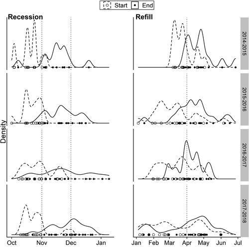
Relative to the MassWildlife (2002) WD timing guidelines, 83.1% of WD events were initiated before 1 November, with 8 distinct WD periods that occurred in Wyman in February to April. Six lakes were permitted to initiate recessions in early to mid-October and comprised 35.2% of recession phases started before 1 November and 30% of total recession phases. Stable phase water levels were reached (i.e., recession end) before 1 December for 63.6% of WD events. Lastly, 70.6% of WD periods did not reach reference water levels by 1 April (Figure 7).

Rates

Sequential recession and refill rates varied across lakes and years (Table S3). Annual median recession rates varied from 0.9 to 5.8 cm/d with an overall median of 2.4 cm/d across lakes. Interannual lake variation of median recession rates ranged from 0 to 9.6 cm/d and the highest median recession rates per lake ranged from 1.2 to 12 cm/d with interannual variation ranging from 0 to 9.6 cm/d across all lakes. Overall, the highest recorded recession rates occurred at Onota with 188.4 cm/d, followed by 73.2 cm/d at Wickaboag, and 71.7 cm/d at Otis. During recession phases, water levels also increased, most notably during 2017–2018 when a relatively large precipitation event occurred during the recession phase.

Annual median refill rates varied from 0.9 to 11.6 cm/d across lakes. Lake interannual variation of median refill rates ranged from 0 to 35.4 cm/d with the highest median rate of 35.4 cm/d and the lowest at 0 cm/d. The highest overall refill rates occurred in Stockbridge (315.6 cm/d), Garfield (126 cm/d), and Greenwater (98.4 cm/d). Similar to recession rates, declines in water level occurred during refill phases. Several lakes reached reference pool level after a strong precipitation/melting event in January 2018 and did not attempt water level recession again.

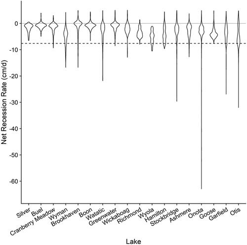
Of the 71 recession periods, 39 possessed net daily recession rates that exceeded the 7.62 cm/d standard (MassWildlife 2002, Figure 8). Several lakes exceeded the 7.62 cm/d standard consistently across WD periods, including Watatic (5.1–30.2% of time), Otis (4.5–27.8% of time), Garfield (8.3–17.1% of time), Brookhaven (1.3–30.1% of time), Wyola (2.2–34.8% of time), and Hamilton (1.8–27.0% of time). Other lakes also exceeded this threshold but not consistently across WD periods (e.g., Onota, Ashmere, Stockbridge), and few lakes did not exceed this threshold overall (Silver, Goose, Boon, Buel). There were 2 recession events in Wyman where median net recession rates exceeded 7.62 cm/d.

Figure 8. Density and range of median daily net recession rates aggregated across WD events per lake. The horizontal dashed line is the recession rate guideline (−7.62 cm/d) from Mattson et al. (2004). Lakes are ordered by ascending WD magnitude.

Metric correlations

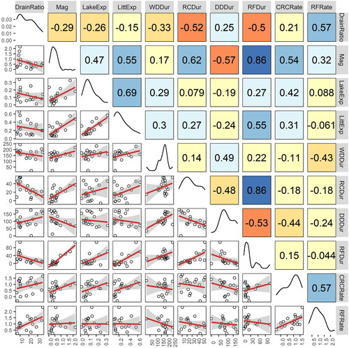
Mean lake WD magnitude was positively correlated with mean lake proportions of lake area exposed and littoral area exposed (Figure 9). Generally, these magnitude metrics were correlated with duration metrics. Notably, magnitude was positively correlated with refill duration and recession duration, and negatively, albeit weakly, with stable phase duration. Duration and magnitude metrics exhibited relatively weaker correlations with recession, including faster recession rates with increasing magnitude. Slower refill rates were correlated with decreasing drainage ratios. Lastly, decreasing drainage ratios were moderately correlated with longer recession and refill durations.

Figure 9. Paired correlations and scatterplot matrix for selected WD metrics in WD lakes (n = 18). Numbers in the upper diagonal are Spearman rank correlation coefficients, with darker colors representing higher negative or positive correlations. Points in scatterplots are interannual medians by lake with linear trendlines and 95% confidence intervals. Diagonal plots represent WD metrics probability density distributions. WD metrics abbreviations and corresponding units are: DrainRatio = drainage ratio (watershed area/lake area), Mag = bihourly mean drawdown phase water level (m), LakeExp = proportion of whole lake area exposed, LittExp = proportion of estimated littoral area exposed, WDDur = duration of entire WD period (d), RCDur = duration of recession phase (d), DDDur = duration of drawdown phase (d), RFDur = duration of refill phase (d), CRCRate = mean cumulative recession rates on a natural log scale (cm/d), RFRate = mean refill rates on a natural log scale (cm/d). Positive changes in cumulative recession rates equate to faster water level declines.

Discussion

Recreational lakes in Massachusetts exhibit wide-ranging WD magnitude, duration, rates, and timing; this study is the first to document this variability over multiple lakes and years, providing essential information for understanding ecological impacts of WD. Most lakes possessed magnitudes of <0.914 m that remained consistent across years; however, differences in lake bathymetry and water quality (i.e., transparency) translated to variable lake and littoral zone exposure. Timing and duration of WD refill phases varied widely across years, suggesting the importance of seasonal-specific precipitation and temperature events. The majority of WD events deviated from Massachusetts timing and recession rate performance standards, which may have unintended ecological impacts to nontarget species (e.g., limited fish spawning habitat, mollusk stranding). Understanding the timing, duration, and rates of WD events in addition to magnitude could be critical for predicting WD impacts on lake ecosystems and managing WDs under climate change.

Potential drivers and ecological implications of WD regimes

Most WD events and lakes had magnitudes less than 0.91 m (0.001–2.16 m, mean = 0.66 m), in line with the guidance of Mattson et al. (2004). Magnitudes that exceeded this standard were found in 5 lakes that obtained local and state government approval. In comparison to hydroelectric lakes, WD in Massachusetts recreational lakes are typically smaller. For example, in hydroelectric lakes of Canada and the US states of Maine and New Hampshire, studies report magnitudes of 0.3–7.2 m (n = 15, mean = 3.0 m, Trottier et al. 2019) and 0.8–10 m (n = 24, White et al. 2011). This suggests WD management context is likely an important driver for magnitude decisions. Many WD regimes are implemented in recreational lakes to dewater shoreline structures (e.g., docks, retaining walls, dams) before ice-on to prevent damage from ice erosion, to reduce nuisance densities of macrophytes that may impede recreational activities (Clayton 1996), or to prevent the spread of nonnative invasive species (Hussner et al. 2017). Thus, most magnitudes are relatively small to correspond to shallow depths of shoreline infrastructure, but larger magnitudes may be conducted to maintain dam integrity (e.g., Otis) or expose a significant portion of a nonnative invasive species like Eurasian watermilfoil (Myriophyllum spicatum; e.g., Mattson et al. 2004).

Recent WD-ecology research derives mostly from hydroelectric and storage lakes that can experience relatively large WD magnitudes (e.g., >2–3 m), which are greater than those observed in our study. Typically, these larger magnitudes have more pronounced impacts to populations and communities (e.g., Haxton and Findlay 2009, White et al. 2011). However, even relatively small WD magnitudes can have substantial ecological impacts. For example, within a subset of the current study lakes, Carmignani et al. (2019) found WD regimes with <1 m magnitudes limited freshwater mussel distributions deeper than stable phase water levels, presumably due to their low mobility and susceptibility to desiccation. Also, short pulses of large and rapid water level recession as observed in our study may expose high mussel densities on shallow benthic shelves (e.g., Onota). Although rare, these relatively extreme events can have a lasting impact to nontarget biota populations (Richardson et al. 2002).

Although WD magnitude was moderately correlated with littoral and lake exposure, these relationships were not strong, emphasizing the importance of morphometry in determining exposure. In shallow lakes or lakes with expansive shallow benthic shelves, relatively small to moderate magnitudes can expose a significant proportion of lakebeds. In contrast, lakes predominantly composed of steep-sided basin slopes show small whole-lake exposure even at high magnitudes observed in this study. Therefore, biotic assemblages occupying shallow uniform depths are more vulnerable to direct WD impacts, such as desiccation and freezing, compared to biotic assemblages distributed along moderate to high sloping lake basins.

Similarly, narrow littoral zones are more susceptible to exposure even at small WD magnitudes because of a lake’s bathymetry (Duarte and Kalff 1990). Nutrient availability and factors that influence water transparency, including phytoplankton and nonalgal suspended solids (Brezonik et al. 2019), will affect littoral zone depth boundaries (i.e., macrophyte colonization) and hence littoral zone exposure. Because littoral zones can provide disproportionately high energy and habitat resources for a diversity of consumers across lake morphometries (Vander Zanden et al. 2011), it is important to estimate littoral zone exposure. Although deep and steep-sided lake morphometries may be less sensitive to overall lake area exposure, valuable benthic-littoral habitat and energy resources are naturally constrained to relatively small areas (Vadeboncoeur et al. 2008) and hence are particularly susceptible to regulated water levels (Eloranta et al. 2018). Even at WD magnitudes of <0.91 m, large proportions of littoral zone habitat were exposed in our study. Accurate estimation of lake and littoral exposure areas will require fine-scaled bathymetry data to generate area exposed and volume lost and will require depth estimations of littoral zone boundaries during summer months.

Typically, WD periods recorded in our study lasted >120 d, such that water levels were receding, refilling, or in stable phases for most of the nonsummer months (e.g., Oct to Apr–Jun). Although entire WD period duration and magnitude were weakly correlated, recession and refill phase durations were moderately to strongly correlated, indicating that more time is needed to reach target stable drawdown water levels and especially summer pool levels. Consequently, stable phase water levels are maintained for shorter durations with increasing magnitudes. These patterns can be attributed to variable interlake WD management decisions to maintain stable water levels up to different dates, and reflect interlake hydrogeomorphic differences (i.e., inflows, outflows, residence time) in response to precipitation events. This is supported by drainage ratio correlations with refill and recession durations, and refill rates in our study that suggest inflows and lake water storage mediate WD regimes.

The timing of WD phases resulted in timing that did not meet the recommendations of the MassWildlife (2002) standards. The majority of WD events were initiated before the 1 November guideline and reached reference pool levels after 1 April. In contrast, the majority of WD recessions ended by the beginning of December, per recommendation; however, this might be the result of relatively early WD initiation dates. Recessions were predominantly initiated before 1 November across years, which suggests lake managers largely dictate and control recession starts. Of the 18 WD lakes, 6 lakes had special performance conditions to initiate water level recession before the 1 November guideline in early and mid-October. Potential reasons for intentional early start dates include meeting target stable phase water levels before ice-on, given Massachusetts state guidelines on downstream flows and in-lake recession rates, and permitting shoreline property maintenance for shoreline residents. Reaching stable phase water levels before ice-on enables targeted benthic areas for macrophyte control to dewater and become exposed to freezing temperatures. Additionally, continued water level drawdown after ice-on can be a safety concern for winter ice recreational activities (Mattson et al. 2004).

The higher interannual variability for the timing of recession end and for refill start and end dates implies less water level control and more influence of environmental factors such as precipitation and ice melt. For example, sustained cold winter temperatures into late March and April of the 2014–2015 winter synchronously delayed refill phases into mid-April to May across many of our study lakes. In contrast, the timing of the start of refill phases and reaching normal pool levels in 2017–2018 was highly variably across lakes. Furthermore, longer refill durations and slower refill rates correlated with decreasing drainage ratios indicate that lake inflows likely influence the timing to meet summer pool levels. Thus, WD phase timing differences among lakes and between years demonstrate the interaction between different WD management practices and lake water budgets.

Since the MassWildlife (2002) guidelines are to help minimize ecological impacts, the general incongruity with timing standards may have ongoing negative ecological effects. The 1 April refill guideline is in part to ensure access to critical shallow-water spawning habitat for spring spawning species (MassWildlife 2002) such as yellow perch, chain pickerel, and northern pike (Esox lucius). Impacts to annual recruitment will depend on the amount of spawning habitat available below drawdown water levels and the disturbance to eggs from fluctuating water levels and wave action (Larson et al. 2016). Future investigations can help assess the availability of spawning habitat (e.g., water temperature, substrate) under different refill scenarios (Papenfuss et al. 2018) and for different fish species that require different spawning substrates. The 1 November recession start guideline delays WD until colder conditions to help prevent in-lake and downstream fish kills resulting from warm, poorly oxygenated water, particularly in shallow, macrophyte-dominated lakes (MassWildlife 2002), but more research is warranted to assess the potential for fish kills. Recession initiation dates before 1 November, by contrast, may benefit benthic species susceptible to exposure. Warmer water temperatures in mid-October could allow for more efficient movement of benthic organisms (e.g., mussels, gastropods), given that recession rates are not extreme. Additionally, earlier recession initiation could enable amphibians and turtles to select overwintering benthic areas that would remain submerged during a drawdown and prevent winterkill events. Lake management will need to consider and balance these potential impacts, given their downstream and lake community composition. Overall, more research could help assess the effects of variable timing on nontarget biota and habitat to help refine WD performance timing guidelines.

Recession and refill rates were similar across most lakes and years in our study; however, the ranges of rates had several key insights. First, we documented relatively extraordinary rates within a few recession and refill phases. For example, we observed maximum net recession rates >25 cm/d for 4 recession phases reaching up to 62.9 cm/d. Second, recession phases often contained rates ≥7.62 cm/d, the MassWildlife (2002) guideline. Although, the percentage of these rates largely composed a minority of rate records, several lakes consistently fell within or exceeded the recession rate guideline across WD periods. Few studies have investigated the effect of recession rates on ecological responses, but low-mobility organisms like freshwater mussels are particularly susceptible to rapid dewatering. Galbraith et al. (2015) found most mussels were stranded under 4 cm/d and 8 cm/d recession rates but with variable species-specific mortality after stranding. Given that many WD events in the current study possessed net daily recession rates >4 cm/d, increases in magnitude with similar recession rates will likely impact existing mussel assemblages, for which the distributions are already restricted by ongoing WD regimes (Carmignani et al. 2019). Also, rapid recession rates may trap fish in shallow pools, leading to mortality via stranding or because of stressful overwintering conditions (Nagrodski et al. 2012). More field-based studies are needed to estimate the effect of typical recession and extreme recession rates on littoral communities. Furthermore, more research is needed to estimate the impact of high outflows to downstream communities associated with WD recession phases, as these flow patterns are likely atypical of natural streamflows during fall months.

WD management implications

The level of annual water level fluctuation is determined by a lake’s water budget (e.g., inflows, outflows, residence time, evapotranspiration), and can be coarsely predicted by drainage ratios such that lakes that comprise an increasing percentage of watershed area will have smaller water level magnitudes (Keto et al. 2008). Based on our results, we hypothesize larger WD magnitudes in lakes with smaller drainage ratios restrict control on the timing, duration, and rates of recession and refill phases because of higher dependency on local precipitation and temperature events as compared to smaller magnitudes in lakes with larger drainage ratios. Therefore, larger WD magnitude regimes with small drainage ratios may have more difficulty meeting WD performance standards for timing and rates. To help balance WD management goals and lake ecological integrity, simulating WD magnitude scenarios under various water budget conditions can help estimate the duration, timing, and rates of WD phases needed to meet or define performance standards. Furthermore, the use of easily determined hydrogeomorphic metrics like drainage ratios can help classify the hydrological status of lakes as developed in Finland’s hydroelectric lakes (Keto et al. 2008). Further research could lead to more detailed hydrological classification of lakes and potentially adapt specific WD performance guidelines according to hydrological classification.

The effectiveness of WD regimes as a macrophyte control strategy in drawdown exposure zones strongly depends on winter weather conditions and the resistance of target species to freezing and desiccation (Cooke 1980). Most WDs monitored in this study were initiated in October, reached target water levels before or in the beginning of December, likely before ice-on, and were refilled in April. This timing and duration allow ample exposure to rhizome-damaging conditions. Lonergan et al. (2014) experimentally found that sediment temperatures at −5 C sustained for ≥24 h, or below a sediment water content threshold for ≥48 h, prevented regrowth of Eurasian watermilfoil, a widespread invasive species in the Northeast. However, the presence of ice and snow cover concurrent with freezing and desiccated soil will dictate the level of rhizome mortality (Lonergan et al. 2014). Early freezing of exposed lakebed followed by snow cover can sustain frozen soil conditions that may result in effective macrophyte rhizome mortality. In contrast, snow cover before the onset of freezing temperatures can effectively insulate sediment above freezing and regulate freeze–thaw cycles (Huntington et al. 2009 and references therein). Thus, sufficient time is needed to allow sediment dewatering before ice formation, along with consecutive subzero freezing days to control susceptible nuisance species. Monitoring of exposed soil temperature and moisture and of ice and snow cover durations during WD periods could help determine the timing of refill once macrophyte mortality conditions are met and the lake is ice-free (Lonergan et al. 2014). Additionally, incorporating fine-scale estimates of bathymetry could help identify benthic areas of high topographic heterogeneity that possess variable moisture and temperature conditions, and hence may be less vulnerable to macrophyte mortality.

Likely changes in lake water level regimes from climate change are a top concern among lake management stakeholders (Magee et al. 2019). Climate change is projected to increase winter temperatures, increase winter rainfall, reduce the extent and duration of snow cover, increase the frequency of short-term droughts, and shift the timing of spring floods in the northeastern United States (Hayhoe et al. 2008, Huntington et al. 2009). Additionally, the current trend of earlier ice-out dates (Hodgkins et al. 2002) is expected to continue in the future, along with the potential of shorter ice cover durations and reduced ice thickness (Huntington et al. 2009).

These projected changes pose challenges to the use of WD regimes as a macrophyte control strategy that also minimizes ecological impacts and maintains recreational value. Specifically, warmer and wetter winters may limit macrophyte mortality by keeping exposed sediment above mortality threshold temperatures and by keeping sediments moist from rainfall and associated water level fluctuations. Another major concern associated with climate change is delayed or incomplete refill to reference pool levels because of a spring drought (Magee et al. 2019). In several lakes in Connecticut, McDowell (2012) documented refill phases that did not reach summer pool levels until mid to late May, as a result of a springtime drought in 2012. Delayed refill extending into summer months could also decrease recreational opportunities for boating and angling (Miranda and Meals 2013) and may decrease lakefront property values (Hanson et al. 2002).

Anticipation of climate-related changes in precipitation and temperature regimes could help guide WD management strategies that adjust the magnitude, duration, and even frequency of WDs to sustain ecological integrity and maintain recreational value. Heterogeneous watershed characteristics (e.g., land use and cover, slope, drainage density) and lake-specific factors (morphometry, residence time) that regulate lake water levels (Molinos and Donohue 2014) could help determine lake-specific adaptation strategies for WD regime management (Magee et al. 2019).

Data needs and conclusions

The scarcity of lake water level records and water level monitoring efforts poses a large challenge to assessing WD impacts on lake ecosystems and understanding the role of anthropogenic stressors interacting with natural controls (e.g., climate change, watershed land cover, lake morphometry). Increased monitoring of lake levels at ecologically relevant temporal resolutions and scales is needed to understand a lake’s natural hydrological character, and to help explain current and future ecological patterns (Magee et al. 2019). Our bihourly measurements of lake water levels enabled the documentation of short-term extreme events (e.g., high recession rates) and captured the overall variability of WD regimes within and between years. Predicted climate changes suggest that winter water level regulation may progressively carry over into summer months (Magee et al. 2019). To understand the ecological effects of such a shift, we strongly recommend that water levels be monitored year-round, as recent evidence suggests summer water level fluctuations impact water quality more (e.g., cyanobacteria blooms; Bakker and Hilt 2016) than winter drawdowns (Elchyshyn et al. 2018). Integrating knowledge of the natural range of variability of unregulated lake levels over long time scales (i.e., decades; Hofmann et al. 2008, Molinos et al. 2015) could help to predict future water level changes in regulated lakes within similar hydromorphic characteristics and direct management to mitigate and anticipate related water quality issues (Lisi and Hein 2019). We also need increased modeling efforts to understand the drivers and patterns of lake water level fluctuations across unregulated and regulated water level regimes and lake types (e.g., drainage, seepage) to help us define the natural range of water level fluctuations and set WD management expectations (Magee et al. 2019). Application of recently developed models can improve our understanding of lake water budgets at local and regional scales and help to estimate the hydrological impacts of varying WD regimes in combination with watershed land cover and land use (Hanson et al. 2018). Knowledge of fundamental lake characteristics including lake morphometry, water transparency, nutrient status, and watershed hydrogeomorphic attributes and how those characteristics control in-lake abiotic and biotic dynamics can help provide context for WD management and its effectiveness in the face of ongoing climate change.

Acknowledgments

We thank the numerous technicians and volunteers who made this work possible, including Kate Stankiewicz, Ian Weishar, Sean Young, Gillian Gundersen, Tansy Remiszewski, Alex Groblewski, Renee Bouldin, Alex Ahlquist, Corey Wrinn, Emily Thomas, and Emily Lozier. JC thanks the Organismic and Evolutionary Biology program at the University of Massachusetts Amherst for support. We thank the Massachusetts Department of Conservation and Recreation for access to water level records. This article was greatly improved as a result of reviews by Phillip Kaufmann and 3 anonymous reviewers. Any use of trade, firm, or product names is for descriptive purposes only and does not imply endorsement by the US government.

Additional information

Funding

This research was funded by the Massachusetts Division of Fisheries and Wildlife.

References

- Bakker ES, Hilt S. 2016. Impact of water-level fluctuations on cyanobacterial blooms: options for management. Aquat Ecol. 50(3):485–414. doi:https://doi.org/10.1007/s10452-015-9556-x.
- Brezonik PL, Bouchard RW, Jr., Finlay JC, Griffin CG, Olmanson LG, Anderson JP, Arnold WA, Hozalski R. 2019. Color, chlorophyll a, and suspended solids effects on Secchi depth in lakes: implications for trophic state assessment. Ecol Appl. 29(3). doi:https://doi.org/10.1002/eap.1871.
- Carmignani JR, Roy AH. 2017. Ecological impacts of winter water level drawdowns on lake littoral zones: a review. Aquat Sci. 79(4):803–824. doi:https://doi.org/10.1007/s00027-017-0549-9.
- Carmignani JR, Roy AH, Hazelton PD, Giard H. 2019. Annual winter water level drawdowns limit shallow ‐ water mussel densities in small lakes. Freshw Biol. 64(8):1519–1533. doi:https://doi.org/10.1111/fwb.13324.
- Clayton JS. 1996. Aquatic weeds and their control in New Zealand lakes. Lake Reserv Manag. 12(4):477–486. doi:https://doi.org/10.1080/07438149609354288.
- Cooke GD. 1980. Lake level drawdown as a macrophyte control technique. J Am Water Resour Assoc. 16(2):317–322. doi:https://doi.org/10.1111/j.1752-1688.1980.tb02397.x.
- Duarte CM, Kalff J. 1990. Patterns in the submerged macrophyte biomass of lakes and the importance of the scale of analysis in the interpretation. Can J Fish Aquat Sci. 47(2):357–363. doi:https://doi.org/10.1139/f90-037.
- Elchyshyn L, Goyette JO, Saulnier-Talbot É, Maranger R, Nozais C, Solomon CT, Gregory-Eaves I. 2018. Quantifying the effects of hydrological changes on long-term water quality trends in temperate reservoirs: insights from a multi-scale, paleolimnological study. J Paleolimnol. 60(3):361–379. doi:https://doi.org/10.1007/s10933-018-0027-y.
- Eloranta AP, Finstad AG, Helland IP, Ugedal O, Power M. 2018. Hydropower impacts on reservoir fish populations are modified by environmental variation. Sci Total Environ. 618:313–322. doi:https://doi.org/10.1016/j.scitotenv.2017.10.268.
- [ESRI] Environmental Systems Research Institute. 2015. ArcGIS Desktop: Release 10.3.1. Redlands (CA): Environmental Systems Research Institute.
- Galbraith HS, Blakeslee CJ, Lellis WA. 2015. Behavioral responses of freshwater mussels to experimental dewatering. Freshw Sci. 34(1):42–52. doi:https://doi.org/10.1086/679446.
- Griffith GE, Omernik JM, Bryce SA, Royte J, Hoar WD, Homer JW, Keirstead D, Metzler KJ, Hellyer G. 2009. Ecoregions of New England (2 sided color poster with map, descriptive text, summary tables, and photographs). Reston (VA): U.S. Geological Survey. Scale 1:1,325,000.
- Hanson TR, Hatch LU, Clonts HC. 2002. Reservoir water level impacts on recreation, property, and nonuser values. J Am Water Resour Assoc. 38(4):1007–1018. doi:https://doi.org/10.1111/j.1752-1688.2002.tb05541.x.
- Hanson ZJ, Zwart JA, Vanderwall J, Solomon CT, Jones SE, Hamlet AF, Bolster D. 2018. Integrated, regional-scale hydrologic modeling of inland lakes. J Am Water Resour Assoc. 54(6):1302–1324. doi:https://doi.org/10.1111/1752-1688.12688.
- Haxton TJ, Findlay CS. 2009. Variation in large-bodied fish-community structure and abundance in relation to water-management regime in a large regulated river. J Fish Biol. 74(10):2216–2238. http://www.ncbi.nlm.nih.gov/pubmed/20735549. doi:https://doi.org/10.1111/j.1095-8649.2009.02226.x.
- Hayhoe K, Wake C, Anderson B, Liang X-Z, Maurer E, Zhu J, Bradbury J, DeGaetano A, Stoner AM, Wuebbles D. 2008. Regional climate change projections for the Northeast U.S. Mitig Adapt Strateg Glob Change. 13(5-6):425–436. doi:https://doi.org/10.1007/s11027-007-9133-2.
- Hellsten SK. 1997. Environmental factors related to water level regulation — a comparative study in northern Finland. Boreal Environ Res 2:345–367.
- Hill NM, Keddy PA, Wisheu IC. 1998. A hydrological model for predicting the effects of dams on the shoreline vegetation of lakes and reservoirs. Environ Manage. 22(5):723–736. doi:https://doi.org/10.1007/s002679900142.
- Hirsch PE, Eloranta AP, Amundsen P-A, Brabrand Å, Charmasson J, Helland IP, Power M, Sánchez-Hernández J, Sandlund OT, Sauterleute JF, et al. 2017. Effects of water level regulation in alpine hydropower reservoirs: an ecosystem perspective with a special emphasis on fish. Hydrobiologia 794(1):287–301. doi:https://doi.org/10.1007/s10750-017-3105-7.
- Hodgkins GA, James ICIC, Huntington TG. 2002. Historical changes in lake ice-out dates as indicators of climate change in New England, 1850-2000. Int J Climatol. 22(15):1819–1827. doi:https://doi.org/10.1002/joc.857.
- Hofmann H, Lorke A, Peeters F. 2008. Temporal scales of water-level fluctuations in lakes and their ecological implications. Hydrobiologia 613(1):85–96. doi:https://doi.org/10.1007/s10750-008-9474-1.
- Huntington TG, Richardson AD, Mcguire KJ, Hayhoe K. 2009. Climate and hydrological changes in the northeastern United States: recent trends and implications for forested and aquatic ecosystems. Can J For Res. 39(2):199–212. doi:https://doi.org/10.1139/X08-116.
- Hussner A, Stiers I, Verhofstad MJJM, Bakker ES, Grutters BMC, Haury J, van Valkenburg JLCH, Brundu G, Newman J, Clayton JS, et al. 2017. Management and control methods of invasive alien freshwater aquatic plants: a review. Aquat Bot. 136:112–137. doi:https://doi.org/10.1016/j.aquabot.2016.08.002.
- Kennedy RH. 2005. Toward integration in reservoir management. Lake Reserv Manag. 21(2):128–138. doi:https://doi.org/10.1080/07438140509354422.
- Keto A, Tarvainen A, Marttunen M, Hellsten S. 2008. Use of the water-level fluctuation analysis tool (Regcel) in hydrological status assessment of Finnish lakes. Hydrobiologia 613(1):133–142. doi:https://doi.org/10.1007/s10750-008-9478-x.
- Krivoruchko K. 2012. Empirical Bayesian Kriging. Redlands (CA): ESRI. [cited 2016 November 10]. www.esri.com/NEWS/ARCUSER/1012/files/ebk.pdf.
- Larson JH, Staples DF, Maki RP, Vallazza JM, Knights BC, Peterson KE. 2016. Do water level fluctuations influence production of walleye and yellow perch young-of-year in large northern lakes? North Am J Fish Manag. 36(6):1425–1436. doi:https://doi.org/10.1080/02755947.2016.1214645.
- Leppo EW, Lincoln AR, Stamp J, Van Sickle J. 2017. ContDataQC: quality control (QC) of continuous monitoring data. R package version 2.0.2.9001. https://github.com/leppott/ContDataQC.
- Linløkken AN, Sandlund OT. 2016. Recruitment of sympatric vendace (Coregonus albula) and whitefish (C. lavaretus) is affected by different environmental factors. Ecol Freshw Fish. 25(4):652–663. doi:https://doi.org/10.1111/eff.12243.
- Lisi PJ, Hein CL. 2019. Eutrophication drives divergent water clarity responses to decadal variation in lake level. Limnol Oceanogr. 64(S1):S49–S59. doi:https://doi.org/10.1002/lno.11095.
- Lonergan T, Marsicano L, Wagener M. 2014. A laboratory examination of the effectiveness of a winter seasonal lake drawdown to control invasive Eurasian watermilfoil (Myriophyllum spicatum). Lake Reserv Manag. 30(4):381–392. doi:https://doi.org/10.1080/10402381.2014.954736.
- Magee MR, Hein CL, Walsh JR, Shannon PD, Zanden JV, Campbell TB, Hansen GJA, Laliberte GD, Parks TP, Sass GG, et al. 2019. Scientific advances and adaptation strategies for Wisconsin lakes facing climate change. Lake Reserv Manag. 35:364–381. doi:https://doi.org/10.1080/10402381.2019.1622612.
- [MassWildlife] Massachusetts Division of Fisheries and Wildlife. 2002. Drawdown performance standards for the protection of fish and wildlife resources. Westborough (MA): MassWildlife.
- Mattson MD, Godfrey PJ, Barletta RA, Aiello A. 2004. Eutrophication and aquatic plant management in Massachusetts final generic environmental impact report. Amherst (MA): Executive Office of Environmental Affairs Commonwealth of Massachusetts.
- McDowell CP. 2012. Winter drawdown effects on swim-up date and growth rate of age-0 fishes in Connecticut [master’s thesis]. Storrs (CT): University of Connecticut.
- Miranda LE, Meals KO. 2013. Water levels shape fishing partcipation in flood-control reservoirs. Lake Reserv Manag. 29(1):82–86. doi:https://doi.org/10.1080/10402381.2013.775200.
- Miranda LE, Spickard M, Dunn T, Webb KM, Aycock JN, Hunt K. 2010. Fish habitat degradation in U.S. reservoirs. Fisheries 35(4):175–184. doi:https://doi.org/10.1577/1548-8446-35.4.175.
- Mjelde M, Hellsten S, Ecke F. 2013. A water level drawdown index for aquatic macrophytes in Nordic lakes. Hydrobiologia 704(1):141–151. doi:https://doi.org/10.1007/s10750-012-1323-6.
- Molinos JG, Donohue I. 2014. Downscaling the non-stationary effect of climate forcing on local-scale dynamics: the importance of environmental filters. Clim Change. doi:https://doi.org/10.1007/s10584-014-1077-4.
- Molinos JG, Viana M, Brennan M, Donohue I. 2015. Importance of long-term cycles for predicting water level dynamics in natural lakes. PLOS One. 10(3):e0119253. doi:https://doi.org/10.1371/journal.pone.0119253.
- [MRLC] Multi-Resolution Land Characteristics Consortium. 2018. National land cover database 2011 (NLCD 2011). Multi-Resolution Land Characteristics Consortium; [cited 1 Mar 2014]. https://data.nal.usda.gov/dataset/national-land-cover-database-2011-nlcd-2011.
- Nagrodski A, Raby GD, Hasler CT, Taylor MK, Cooke SJ. 2012. Fish stranding in freshwater systems: sources, consequences, and mitigation. J Environ Manage. 103:133–141. doi:https://doi.org/10.1016/j.jenvman.2012.03.007.
- Papenfuss JT, Cross T, Venturelli PA. 2018. A comparison of the effects of water-level policies on the availability of walleye spawning habitat in a boreal reservoir. Lake Reserv Manag. doi:10.1080/10402381.2018.1448021.
- Perlelberg D, Radomski P, Simon S, Carlson K, Knopik J. 2016. Minnesota lake plant survey manual, for use by MNDNR Fisheries Section and EWR Lake Habitat Program. Brainerd (MN): Minnesota Department of Natural Resources, Ecological and Water Resources Division. 128 pages including Appendices A-E.
- R Core Team. 2017. R: A language and environment for statistical computing. Vienna (Austria): R Foundation for Statistical Computing. https://www.R-project.org/.
- Richardson SM, Hanson JM, Locke A. 2002. Effects of impoundment and water-level fluctuations on macrophyte and macroinvertebrate communities of a dammed tidal river. Aquat Ecol. 36(4):493–510. doi:https://doi.org/10.1023/A:1021137630654.
- Stamp J, Hamilton A, Craddock M, Parker L, Roy AH, Isaak DJ, Holden Z, Passmore M, Bierwagen BG. 2014. Best practices for continuous monitoring of temperature and flow in wadeable streams EPA/600/R-13/170F. Washington (DC): U.S. Environmental Protection Agency, Office of Research and Development, National Center for Environmental Assessment, Global Change Research Program.
- Sutela T, Aroviita J, Keto A. 2013. Assessing ecological status of regulated lakes with littoral macrophyte, macroinvertebrate and fish assemblages. Ecol Indic. 24:185–192. doi:https://doi.org/10.1016/j.ecolind.2012.06.015.
- Trottier G, Embke H, Turgeon K, Solomon C, Nozais C, Gregory-Eaves I. 2019. Macroinvertebrate abundance is lower in temperate reservoirs with higher winter drawdown. Hydrobiologia 834(1):199–211. doi:https://doi.org/10.1007/s10750-019-3922-y.
- Vadeboncoeur Y, Peterson G, Vander Zanden MJ, Kalff J. 2008. Benthic algal production across lake size gradients: interactions among morphometry, nutrients, and light. Ecology 89(9):2542–2552. doi:https://doi.org/10.1890/07-1058.1.
- Vander Zanden MJ, Vadeboncoeur Y, Chandra S. 2011. Fish reliance on littoral-benthic resources and the distribution of primary production in lakes. Ecosystems 14(6):894–903. doi:https://doi.org/10.1007/s10021-011-9454-6.
- Wantzen KM, Junk WJ, Rothhaupt K-O. 2008a. An extension of the floodpulse concept (FPC) for lakes. Hydrobiologia 613(1):151–170. doi:https://doi.org/10.1007/s10750-008-9480-3.
- Wantzen KM, Rothhaupt K-O, Mörtl M, Cantonati M, G.-Tóth L, Fischer P. 2008b. Ecological effects of water-level fluctuations in lakes: an urgent issue. Hydrobiologia 613(1):1–4. doi:https://doi.org/10.1007/s10750-008-9466-1.
- White MS, Xenopoulos MA, Metcalfe RA, Somers KM. 2011. Water level thresholds of benthic macroinvertebrate richness, structure, and function of boreal lake stony littoral habitats. Can J Fish Aquat Sci. 68(10):1695–1704. doi:https://doi.org/10.1139/f2011-094.
- Whittier TR, Larsen DP, Peterson SA, Kincaid TM. 2002. A comparison of impoundments and natural drainage lakes in the Northeast USA. Hydrobiologia 470(1/3):157–171. doi:https://doi.org/10.1023/A:1015688407915.
- Zohary T, Ostrovsky I. 2011. Ecological impacts of excessive water level fluctuations in stratified freshwater lakes. IW 1(1):47–59. doi:https://doi.org/10.5268/IW-1.1.406.