A high temperature turbine blade heat transfer multilevel design platform

Abstract

In this work, a fast and efficiently design method has been introduced. This design process consists of the overall design and the detailed design. For the overall design, one-dimensional pipe-network computations are employed to obtain several design cases quickly at the beginning. Meanwhile the solid domain geometry and mesh with cooling structures, i.e., film holes, impingement holes, and ribs have been generated to carry out three-dimensional (3-D) heat conduction calculations. Based on the above, a detailed design has been performed by 3-D conjugate heat transfer calculations. The results show that both the average temperature and the mass flow maximum errors between the pipe-network and 3-D conjugate heat transfer calculations are about 10%. In this article, the cooling structure of a gas turbine blade is designed with this platform. The final design results show that the maximum dimensionless temperature on the blade surface is 0.813, i.e., lower than the design requirement. The dimensionless mass flow rate in the first cooling inlet is 0.0168, and the mass flow rate in the secondary inlet is 0.0231.

1. Introduction

Because of the high demand of output power and efficiency in gas turbines, the turbine inlet temperature is increased continuously. Therefore, the cooling system of turbines must be designed to make sure that the maximum temperature of the blade surface is under the allowable metal temperature. To achieve this goal, the cooling system studied should cover two aspects: a highly efficient cooling technology (film cooling, internal cooling, and new technology); a fast and efficient design method.

The current research is mainly focusing on highly efficient cooling technologies, such as film cooling, impingement, ribs, and pin-fins. The film cooling technology is characterized by the hole which is located at the body of the blade and allows the coolant to pass from an internal passage to the external surface. The coolant removes the heat from the blade surface to protect the blade. Many papers [1–3] have already presented detailed reviews. Apart from the film cooling, the internal cooling also plays an important role in the cooling technology. The internal cooling technology includes impingement, ribs, and pin-fins. Impingement has the highest heat transfer coefficient compared with other internal cooling technologies. However, the impingement may weaken the structural strength [4]. Therefore, the impingement usually is used at the leading edge where the thermal load is highest. Ribs are usually located at the opposite wall of the internal cooling passage to enhance the heat transfer. The rib height, pitch, and angle influence the heat transfer coefficient [5–7]. At the trailing edge, it is necessary to enhance the heat transfer and structural strength and consequently pin fins are used. Many works investigated the effect of the shape, height to diameter, and arrangement on the heat transfer [8–11]. In addition to the existing methods, dimples [12–14], impingement [15–17], and porous materials [18,19] have been gradually studied.

Compared to the cooling structure, fewer papers have been published concerning the cooling design method. At present, the pipe network calculation is the main method in the turbine blade heat transfer design. Damerow et al. [20] compared experimental results with results of a compressible flow network analysis. The results showed that the pipe network has good ability to predict the heat transfer and friction factor. Meitner [21] used the pipe-network to predict the coolant flow and heat transfer in a turbomachinery. In that study, the one-dimensional (1-D) momentum and energy equations were used to calculate the temperature, pressure, velocity, and heat transfer coefficient. The results showed that the pipe-network method could present a quick and accurate solution of the turbine heat transfer. The limitation of this code was that it only calculated the stationary state in a radial turbomachinery. Carcasci and Facchini [22] developed a code which could simulate the cooling effect on the stator blade in a gas turbine. Impingement flow, pin fins, and film holes were considered in this code. The results showed that the simulation results corresponded to the experimental results. Off-design performance was also calculated. Kumar et al. [23,24] improved the pipe-network code which was based on the Meitner work [21]. The new code was able to calculate the flow and heat transfer in the rotor blade. Kutz and Speer [25] used the pipe-network model to calculate the secondary air system. The accuracy of the pipe-network model was verified by the experimental results. Talya et al. [26,27] considered the internal cooling technology and film cooling together in a turbine blade. Both the blade geometry and cooling structure were optimized. In this code, the blade was divided into several spanwise sections. Bezier–Bernstein polynomial was used to describe the section geometry. The Kreisselmeier–Steinhauser function approach was used to optimize the geometry. After the optimization, the maximum temperature and average temperature were decreased. Jelisavcic et al. [28] combined the pipe-network model with a multiobjective design optimization to optimize a Pratt and Whitney gas turbine. The cross-sectional areas, hydraulic diameters, ribs were optimized to minimize the coolant flow rate, and pressure losses. Finally, the best parameters were found based on the pipe-network and optimization. Martin and Dulikravich [29] developed a three-dimensional (3-D) internal cooling network based on the Jelisavcic et al. work [28]. The Pratt and Whitney F100 second blade was used to verify the code. The optimization found that the cooling effectiveness achieved 5% improvement. Yu et al. [30] presented a methodology of parametric modeling design and a fully automated integration strategy for the internal cooling turbine blade. The aerodynamic efficiency was increased by 0.6%, the maximum temperature was reduced by 2.4%, and the average temperature in the blade surface was reduced by 1.42%.

According to the existing methods of pipe-network, the codes were only used to calculate the heat transfer and flow in the stator or rotor. The single 1-D design is not enough to estimate the scheme consequences accurately, and it is not convenient to obtain the geometry model and mesh for 3-D heat conduction calculations or conjugate heat transfer. The present work develops a multilevel cooling structure design process, which embodies two main modules: overall design module and detail design module, to absorb the advantages of the pipe-network method and 3-D conjugate heat transfer simulations. The platform cannot only realize a design guide and highly accurate thermal calculations, but also gain the geometry model parameters and mesh automatically and thereby reducing design time significantly. With this design process, the cooling structure of a gas turbine blade is designed and the result meets the requirement.

2. Problem description and boundary conditions

2.1. Problem description

In this study, a cooling structure design process of high efficiency, high robustness, and accuracy for gas turbine vane/blade is introduced. A cooling structure for a gas turbine vane/blade with a high inlet temperature greater than 1,600 K is designed with this design process. The mass flow rate, heat transfer characteristics, and flow structures are compared and analyzed. This study is carried out as follows:

First of all, the design process is introduced, and the process, governing equations, different methods are described in detail. This is favorable for understanding of this design process.

Then, a gas turbine blade with a high temperature at the inlet is introduced. The thermal load, i.e., heat transfer coefficient on the blade surface and the gas temperature, is computed by a 3-D CFD approach in the mainstream.

Third, an overall design process is used to generate the geometry of the cooling structure, divide the internal cooling structure into several cooling elements, compute the detail information of cooling elements, i.e., inlet and outlet area, equivalent diameter, heat transfer area, thickness of the wall, heat transfer coefficient, and temperature at the outer wall, conduct the pipe-network calculations, generation of the mesh of the solid domain of the cooling structure, and then, 3-D heat conduction calculations in the solid domain. Two cooling structures with different topologies are designed and compared to achieve a cooling structure with high cooling efficiency.

Finally, a detail design process is conducted to obtain the detail flow field and temperature distributions. 3-D conjugate heat transfer computations are performed to evaluate the detailed temperature distributions and the flow structure. A minor revision of the cooling structure is carried out to increase the cooling efficiency. The results of the mass flow rate distribution, temperature distribution by the scheme design, and detailed design are compared, which is beneficial for engineering applications.

2.2. Introduction of the design process

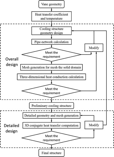
Figure 1 shows the design process. This design process includes the overall design and detailed design. The introduction of all steps is described as follows:

Figure 1. Diagram of the design process.

2.2.1. Scheme design

1. Heat transfer coefficient and the temperature (Initialization data). The function of initialization of the boundary module is to extract the boundary conditions needed for the pipe network calculations from the input files. The input files consist of vane/blade profile data, parameters obtained from CFD calculations of the mainstream, i.e., blade surface pressure, adiabatic wall temperature, and heat flux. Intermediate cooling or film cooling is not considered in the CFD calculations. The definition of the heat transfer coefficient will be discussed later.

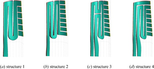
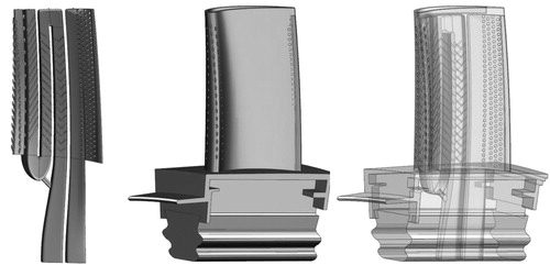
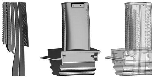
2. Cooling structure geometry generation. To improve the gas turbine performance, the cooling structures of the gas turbine vane/blade become rather complex. This is so as the convenient and rapid cooling structure generation will directly affect the efficiency and quality for the whole design process. To achieve a rapid cooling structure generation, a new cooling structure generation method will be introduced by an in-house code, which is called "the element method." The method is divided into three parts. The first step is to generate the inner and outer walls of the vane or blade, which is based on the thickness distribution of the blade, and the thickness varies with the radial position and chord position. The second step is to carve the cavity into several blocks along the radial and chord directions at the same time, and then, regularly arranged blocks are obtained, each of which is a design element. Each element can simply add different channel types including a straight pipe and an elbow, as shown in Figure 2 for different turbine blade inner cooling channels by the element method. The third step is to add textured cooling structures on different elements, such as pin-fins, film holes, impingement holes, and ribs.

   Figure 2. Different turbine blade inner cooling channels by the element method.

   

3. Preparing the data for the pipe-network calculations. According to the topological structure of elements and boundary conditions, the geometry data and boundary information of each element needed for pipe-network calculations will be extracted and stored by the in-house code. The data obtained are shown in Table 1.

   Table 1. Data for pipe-network.

   Index	Variables	Instruction	Index	Variables	Instruction
   1	nodi	Index of inlet node	16	bg	Length ratio
   2	nodj	Index of outlet node	17	omega	Rate of turning
   3	kindflag	Kind of element	18	hg1	Heat transfer coefficient at the suction side of gas side
   4	area	Area	19	areag1	Heat transfer area at the suction side of gas side
   5	dh	Equivalent diameter	20	tg1	Temperature at the suction side of gas side
   6	leng	Length of the channel	21	deta1	Thickness of solid at suction side
   7	area1	Inlet area	22	hg2	Heat transfer coefficient at the pressure side of gas side
   8	r1	Radial of inlet	23	areag2	Heat transfer area at the pressure side of gas side
   9	area2	Outlet area	24	tg2	Temperature at the pressure side of gas side
   10	r2	Radial of outlet	25	deta2	Thickness of solid at pressure side
   11	areah1	Heat transfer area of suction side of internal	26	lamda	Thermal conductivity of solid domain
   12	areah2	Heat transfer area of pressure side of internal	27	twf	Temperature at the hub side
   13–15	–	Configurations of the cooling element, which is used for the heat transfer and friction factor correlations

4. Pipe-network. In the hierarchical design system, a calculation method, with the abilities of high calculation speed and preliminarily evaluation of the characteristics of the cooling structure design, is needed to guide the overall design. The pipe-network is a 1-D calculation method. As a traditional thermal analysis method of blade cooling structure, it has the advantages of high running speed, less data, and the physical quantities that designers are most concerned about can be obtained, e.g., flow rate, pressure, and blade temperature. Therefore, the designer can calculate several numbers of cooling schemes separately in the scheme design. According to such results, the characteristics of the cooling structure for the vane or blade will be recognized and the direction of modifications will be found.

5. Mesh generation for the solid domain. Because the in-house code can read the geometry data of the cooling structure, which are the outcome of the element method, and then, supplement the relevant parameters of the mesh generation, the solid domain mesh will be completed by an algebraic method. It is convenient for 3-D heat conduction calculations and 3-D conjugate heat transfer calculations and this will further improve the design efficiency.

6. 3-D heat conduction calculation. The distribution of temperature and heat transfer in the inner and outer walls of the vane or blade can be obtained by pipe-network calculations and the mesh of the solid domain can be generated by the mesh generation program. Then, 3-D heat conduction calculations will be carried out. As a follow-up computation, the 3-D heat conduction calculations have the characteristics of higher accuracy. In addition, the designer can gain more detailed information of the temperature distribution. The governing equations will be given later.

2.2.2. Detailed design

After the preliminary cooling structure is obtained, it is necessary to design the cooling structure in detail. First of all, the detailed flow structure and heat transfer should be studied, which cannot be obtained in the scheme design process. Then, the very detailed structure, i.e., the outline of the cooling structure, the detailed layout of the pin fins, ribs, film holes, and dust holes, effects on the flow field and heat transfer of the cooling structure will be analyzed.

1. Detailed geometry generation. After the preliminary cooling structure is obtained, the geometry can be generated, and the detailed structure, such as filet, layout and details of pin fins, ribs, film holes, and dust holes will be designed in this process.

2. Mesh generation. To conduct the 3-D conjugate heat transfer simulations, the mesh needs to be obtained. The mesh in this design process is achieved by the commercial software ANSYS-ICEM. The near wall regions of the flow have prismatic meshes to capture the details of the heat transfer and flow fields.

3. 3-D conjugate heat transfer calculations. The computations of the 3-D conjugate heat transfer calculations are performed using the commercial solver ANSYS-CFX. To reduce the numerical errors, a second-order high-resolution advection scheme and high-resolution turbulence numeric are applied to discretize the governing equations. All predicted quantities are obtained at steady state. The minimum convergence criteria for the continuity equation, velocity, and turbulence quantities are 1e-4 and 1e-7 for the energy equation.

2.3. Solution method

2.3.1. Solution method for pipe-network

1) Governing equation. The governing equation of the pipe-network model contains continuity equation, momentum equation, and energy equation which consider the change of the mass flow rate, the change of the sectional area, transport of heat, transport of energy, friction effects on the flow, and heat transfer. Before the governing equations of the pipe-network were established, these assumptions were made. (1) The flow is 1-D and steady, and the parameters of the air flow vary continuously. (2) The gas follows the ideal gas equation of state. (3) The influence of gravity is ignored. (4) The temperature, pressure, and friction coefficient of the airflow in the unit are evenly distributed.

For the flow in a gas turbine vane or blade, the governing equations of the pipe-network are as follows [31–33].

Continuity equation for the node (the place between the elements which are connected): (1) $$\sum _j{q}_{ij}=0$$(1) Momentum equation: (2) $$\left[1-{\left(\frac{\dot{m}}{A}\right)}^2\frac{RT}{p^2}\right]\frac{dp}{dx}=\left[-2\left(\frac{\dot{m}}{A}\right)\frac{RT}{pA}+\frac{V_{\mathit{injx}}}{A}\right]\frac{d\dot{m}}{dx}-{\left(\frac{\dot{m}}{A}\right)}^2\frac{R}{p}\frac{dT}{dx}+{\left(\frac{\dot{m}}{A}\right)}^2\frac{RT}{pA}\frac{dA}{dx}-\frac{C_f}{2}\frac{RT}{\mathit{pDh}}{\left(\frac{\dot{m}}{A}\right)}^2+r{\mathrm{\Omega }}^2\frac{p}{RT}\frac{dr}{dx}$$(2) Energy equation for the cooling element: (3) $$\left(\dot{m}Cp+\frac{{\dot{m}}^{2}RT}{pA}\frac{\dot{m}R}{pA}\right)\frac{dT}{dx}=\frac{\dot{m}RT}{pA}\frac{\dot{m}RT}{p^{2}A}\frac{dp}{dx}+\dot{m}{\mathrm{\Omega }}^{2}r\frac{dr}{dx}+\frac{\delta Q}{dx}+\frac{{\dot{m}}^{2}RT}{pA}\frac{\dot{\mathit{mRT}}}{p{A}^2}\frac{dA}{dx}$$(3) Energy equation for the node: (4) $$T_i=\frac{\sum _j{Cp}_{ij}\mathrm{m}\mathrm{in}(q_{ij},0)T_{ij}}{\sum _j{Cp}_{ij}\mathrm{m}\mathrm{in}(q_{ij},0)}$$(4) 2) Difference method. (5) $$\left(p_j-p_i\right)E_{ij}=A_{ij}-B_{ij}{\dot{m}}_{ij}^2-D_{ij}{\dot{m}}_{ij}^2-C_{ij}{C}_f{\dot{m}}_{ij}^2$$(5) A first-order difference method is used to discretize the momentum equation as

where (6) $$\begin{array}{c}{A}_{ij}=\left[\frac{p_j+p_i}{R(T_j+T_i)}-\frac{C_1}{2C_p}\right]\frac{r_j^2-r_i^2}{2}{\mathrm{\Omega }}^2\\ B_{ij}=\left[\frac{R(T_j+T_i)}{2(p_j+p_i)}-\frac{C_1{R}^2}{2C_p}\frac{{(T_j+T_i)}^2}{{(p_j+p_i)}^2}\right]\left(\frac{1}{A_j^2}-\frac{1}{A_i^2}\right)-\frac{\dot{q}}{{\dot{m}}_{ij}^3{C}_p}\frac{2L}{Dh}\left(A_j+A_i\right)\\ C_{ij}=\frac{{\dot{m}}_{ij}}{\left|{\dot{m}}_{ij}\right|}\frac{RT}{8Dh}\frac{T_j+T_i}{p_j+p_i}{\left(\frac{1}{A_j}+\frac{1}{A_i}\right)}^2\\ E_{ij}=1-\frac{{\dot{m}}_{ij}^{2}R}{2}\frac{T_j+T_i}{{\left(p_j+p_i\right)}^2}{\left(\frac{1}{A_j}+\frac{1}{A_i}\right)}^2+\frac{C_1{\dot{m}}_{ij}^{2}R}{2C_p}\frac{{(T_j+T_i)}^2}{{(p_j+p_i)}^3}{\left(\frac{1}{A_j}+\frac{1}{A_i}\right)}^2\end{array}$$(6) Also, the energy equation for the cooling element can be simplified to (7) $${\dot{m}}_{ij}\left(h_j^{\mathrm{*}}-\frac{1}{2}{r}_j^2{\mathrm{\Omega }}^2\right)-{\dot{m}}_{ij}\left(h_i^{\mathrm{*}}-\frac{1}{2}{r}_i^2{\mathrm{\Omega }}^2\right)=U_{a1}\left(T_{g1}-T_c\right)+U_{a1}\left(T_{g2}-T_c\right)$$(7) where (8) $$U_{a1}={\left[\frac{1}{h_{g1}{A}_{g1}}+\frac{2\delta }{\lambda (A_{g1}+A_{c1})}+\frac{1}{h_{c1}{A}_{c1}}\right]}^{-1}$$(8) (9) $${U_{a2}=\left[\frac{1}{h_{g2}{A}_{g2}}+\frac{2\delta }{\lambda (A_{g2}+A_{c2})}+\frac{1}{h_{c2}{A}_{c2}}\right]}^{-1}$$(9) 3) Solving method. To reduce the dependence on the initial values, a new iterative algorithm is developed as follows:

First the Eq. (10)(10) $$p_j-p_i=N_{ij}{\dot{m}}_{ij}-M_{ij}$$(10) can be written as (10) $$p_j-p_i=N_{ij}{\dot{m}}_{ij}-M_{ij}$$(10) where $M_{ij}=A_{ij}/E_{ij},$ $N_{ij}=N_{ji}=\left(B_{ij}{q}_{ij}+C_{ij}{C}_f{\dot{m}}_{ij}\right)/E_{ij},$ $M_{ij}=-M_{ji}$

The mass flow rate can be obtained (11) $${\dot{m}}_{ij}=\frac{p_i}{N_{ij}}-\frac{p_j}{N_{ij}}+\frac{M_{ij}}{N_{ij}}$$(11) Then, this equation is inserted into the continuity equation for the node. One finds (12) $$Hp=d$$(12) where H is a coefficient matrix, the diagonal element of the matrix is $H_{ii}=-\sum _{j}1/N_{ij}.$ When a flow element exists between node i and j, then, $H_{ij}=-1/N_{ij}.$ The rest has $H_{ij}=0.$ Conversely, when the node i has a pressure boundary, i.e., inlet or outlet, the $H_{ii}=1$ and $H_{ij}=0.$ The d is a 1-D array with $d_i=\sum _j{M}_{ij}/N_{ij}.$ However, $d_i=p_{bi}$ when the node i has a pressure boundary while it is $d_i=\sum _j{M}_{i\mathrm{j}}/N_{ij}-q_{bi}$ when a mass flow rate boundary is applied. The vector p is the pressure result for each node. After the pressure is obtained, the mass flow rate can be obtained by Eq. (11)(11) $${\dot{m}}_{ij}=\frac{p_i}{N_{ij}}-\frac{p_j}{N_{ij}}+\frac{M_{ij}}{N_{ij}}$$(11) . Then, put the temperature, pressure, mass flow rate are inserted into the solution of the upper equations, and then, it is looped until convergence is reached. Then, all the results can be obtained.

2.3.2. Solution method for 3-D heat conduction calculations

For the 3-D heat conduction calculations, the energy equation for the solid is (13) $$\frac{\partial }{{\partial x}_i}\left(\lambda \frac{\partial \overline{T}}{\partial x_i}\right)=0$$(13) The third boundary condition is used for the inner wall and outer wall of the turbine vane or blade, i.e., temperature and heat transfer coefficient. Then, the temperature on the vane or blade can be obtained.

2.3.3. Solution method for 3-D conjugate heat transfer calculations

In this study, the fluid is considered as compressible. Thus, the governing equations used for this flow are described as follows [34].

Continuity equation (14) $$\frac{\partial \left(\rho {\overline{u}}_i\right)}{\partial x_i}=0$$(14) Momentum equation (15) $$\frac{\partial \left(\rho {\overline{u}}_i{\overline{u}}_j\right)}{\partial x_j}=-\frac{\partial \overline{P}}{\partial x_i}+\frac{\partial }{\partial x_j}\left((\mu +{\mu }_t)\left(\frac{\partial {\overline{u}}_i}{\partial x_j}+\frac{\partial {\overline{u}}_j}{\partial x_i}\right)\right)$$(15) Energy equation for fluid (16) $$C_p{\overline{u}}_i\frac{\partial \rho \overline{T}}{\partial x_i}=\frac{\partial }{\partial x_i}\left(\lambda \frac{\partial \overline{T}}{\partial x_i}\right)-C_p\frac{\partial }{\partial x_i}\left(\frac{{\mu }_t}{{Pr}_t}\frac{\partial \overline{T}}{\partial x_i}\right)$$(16) The computations are carried out by RANS turbulence modeling combined with the kω-SST turbulence model. The kω-SST turbulence model is believed to improve the predictive capability for complex turbulent flows with flow swirling and separation, and it is also claimed to offer the best tradeoff between accuracy and computational demands for the parameters considered [35–38]. Therefore, the kω-SST turbulence model is employed and the following equations according to Ref. [39] are used.

The equation of the turbulent kinetic energy k reads (17) $$\frac{\partial }{\partial x_i}\left(\rho k{u}_i\right)={\tau }_{ij}\frac{\partial u_j}{\partial x_i}-{\beta }^{\mathrm{*}}\rho \omega k+\frac{\partial }{\partial x_i}\left[\right(\mu +{\sigma }_k{\mu }_t\left)\frac{\partial k}{\partial x_i}\right]$$(17) The equation of the dissipation rate ω reads (18) $$\frac{\partial }{\partial x_i}\left(\rho \omega u_i\right)=\frac{\gamma }{v_t}{\tau }_{ij}\frac{\partial u_j}{\partial x_i}-\beta \rho {\omega }^2+\mathrm{}\frac{\partial }{\partial x_i}\left[\right(\mu +{\sigma }_{\omega }{\mu }_t\left)\frac{\partial \omega }{\partial x_i}\right]+2(1-F_1)\frac{\rho {\sigma }_{\omega 2}}{\omega }\frac{\partial k}{\partial x_i}\frac{\partial \omega }{\partial x_i}$$(18) where (19) $$\beta =F_1{\beta }_1+(1-F_1){\beta }_2$$(19) (20) $${\sigma }_{\omega }=F_1{{\sigma }_{\omega }}_1+(1-F_1){{\sigma }_{\omega }}_2$$(20) (21) $${\sigma }_k=F_1{{\sigma }_k}_1+(1-F_1){{\sigma }_k}_2$$(21) (22) $$\gamma =F_1{\gamma }_1+(1-F_1){\gamma }_2$$(22) (23) $${\gamma }_1=\frac{{\beta }_1}{{\beta }^{\mathrm{*}}\mathrm{}}-{\sigma }_{\omega 1}{\kappa }^2/\sqrt{{\beta }^{\mathrm{*}}}$$(23) (24) $${\gamma }_2=\frac{{\beta }_2}{{\beta }^{\mathrm{*}}\mathrm{}}-{\sigma }_{\omega 2}{\kappa }^2/\sqrt{{\beta }^{\mathrm{*}}}$$(24) (25) $$v_t=\frac{{\alpha }_{1}k}{\max ({\alpha }_1\omega ,\mathrm{\Omega }{F}_2)}$$(25) (26) $${\tau }_{ij}={\mu }_t\left(2S_{ij}-\frac{2}{3}\frac{\partial u_k}{\partial x_k}{\delta }_{ij}\right)-\frac{2}{3}\rho k{\delta }_{ij}$$(26) (27) $$S_{ij}=\frac{1}{2}(\frac{\partial u_j}{\partial x_i}+\frac{\partial u_i}{\partial x_j})$$(27) (28) $${\mu }_t=\frac{\rho {\alpha }_{1}k}{\max ({\alpha }_1\omega ,\mathrm{\Omega }{F}_2)}$$(28) (29) $$F_1=\tanh \left({\mathit{arg}}_1^4\right)$$(29) (30) $${\mathit{arg}}_1=\min [\max \left(\frac{\sqrt{k}}{{\beta }^{\mathrm{*}}\omega d},\frac{500v}{d^2\omega }\right),\frac{4\rho {\sigma }_{\omega 2}k}{{CD}_{k\omega }{d}^2}]$$(30) (31) $${CD}_{k\omega }=\max \left(2\rho {\sigma }_{\omega 2}\frac{1}{\omega }\frac{\partial k}{\partial x_i}\frac{\partial w}{\partial x_i},{10}^{-20}\right)$$(31) (32) $$F_2=\tanh \left({\mathit{arg}}_2^2\right)$$(32) (33) $${\mathit{arg}}_2=\max (2\frac{\sqrt{k}}{{\beta }^{\mathrm{*}}\omega d},\frac{500v}{d^2\omega })$$(33) The constants have the values: ${\sigma }_{k1}\mathrm{}$= 0.85,$\mathrm{}{\sigma }_{k2}$= 1 ${\sigma }_{\omega 1}\mathrm{}$= 0.65,$\mathrm{}{\sigma }_{\omega 2}$= 0.856,$\mathrm{}{\beta }_1\mathrm{}$= 0.075,$\mathrm{}{\beta }_2\mathrm{}$= 0.0828,$\mathrm{}{\beta }^{\mathrm{*}}\mathrm{}$= 0.09, ${\alpha }_1=0.31,$ $\kappa =0.41.$

2.4. Pipe-network and CFD validations

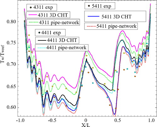
Figure 3 shows the comparison of the temperature distributions at the mid span between the experimental results [40], pipe-network calculations, and 3-D conjugate heat transfer calculations. The test conditions include No. 4311, No. 4411, and No. 5411. It is found that the results of the pipe-network calculations and 3-D conjugate heat transfer calculations are well matching with the experimental results. The calculation results of the pipe-network under No. 3411 conditions show higher accuracy than the 3-D conjugate heat transfer calculations. In summary, many pipe-network calculations and 3-D conjugate heat transfer calculations can be done.

Figure 3. Pipe-network and CFD validation.

2.5. Data reduction

The heat transfer coefficient is defined as: (34) $$\mathrm{h}=\frac{q}{T_{\mathrm{wall}}-T_{\mathrm{in}}}$$(34) where q is the wall heat flux, $T_{\mathrm{wall}}$ is the temperature in the blade surface, $T_{\mathrm{in}}$ is the average static temperature of the inlet.

The dimensionless total pressure $P_t^{\mathrm{*}}$ is defined as: (35) $$P_t^{\mathrm{*}}=\frac{P_t}{P_{\mathrm{tin}}}$$(35) where $P_{\mathrm{tin}}$ is the mass flow average total pressure in the stationary reference frame.

The dimensionless total temperature $T_t^{\mathrm{*}}$ is defined as: (36) $$T_t^{\mathrm{*}}=\frac{T_t}{T_{\mathrm{tin}}}$$(36) where $T_{\mathrm{tin}}$ is the mass flow average total temperature in the stationary reference frame.

The dimensionless mass flow rate $m^{\mathrm{*}}$ is defined as: (37) $$m^{\mathrm{*}}=\frac{m}{m_{\mathrm{de}}}$$(37) where $m_{\mathrm{de}}$ is the mass flow at the inlet of the mainstream.

2.6. Geometry and the boundaries

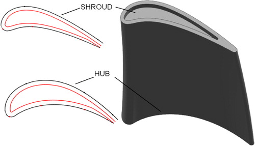
A first stage rotor blade is used to validate the pipe-network. The geometry and boundary conditions come from the aerodynamic design results. The geometries for the different sections are shown in Figure 4a. The design speed of the blade is 17,500 rev/min. The number of blades is 53. The high pressure rotor has a tip-clearance of near 0.5% of the blade span. According to the requirement, the dimensionless mass flow rate of the cooling air is less than 0.0407. For a single blade, the dimensionless maximum temperature of the blade surface is less than 0.8384.

Figure 4. Blade profile and boundary conditions.

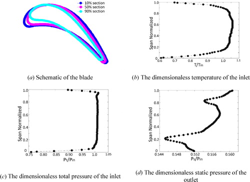
The inlet dimensionless total pressure and dimensionless total temperature are shown in Figures 4b, c. The inlet temperature is far above the permissible temperature of the material. The maximum temperature for the inlet appears at the 65% of the span. Five percent turbulence intensity is applied to the inlet according to the prior study. The outlet dimensionless static pressure is shown in Figure 4d. A constant temperature (1,000 K) is applied on the blade surface to obtain the wall heat flux. The dimensionless total temperature of the cooling air is set to 0.3886. To obtain the pressure distribution and heat flux near the wall, CFD calculations are performed in the mainstream of the blade without internal cooling.

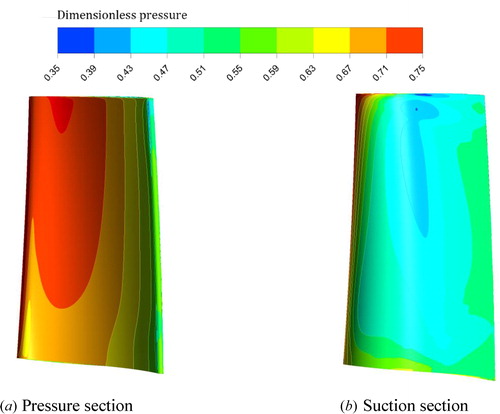
After the simulations, the heat transfer coefficient is shown in Figures 5a, b. It is found that the highest heat transfer coefficient occurs at the leading edge because of the stagnation. For the pressure section, a higher heat transfer coefficient occurs near the blade root and tip. The trailing edge shows higher heat transfer coefficient on the suction side. This might be attributed to the laminar-turbulent boundary layer transition. The highest heat transfer coefficient of the suction side appears at the top of the blade because of the leakage flow. Figure 6 shows the pressure distribution at the blade surface. The pressure distribution can affect the flow rate of the cooing air directly.

Figure 5. The heat transfer coefficient on the blade surface.

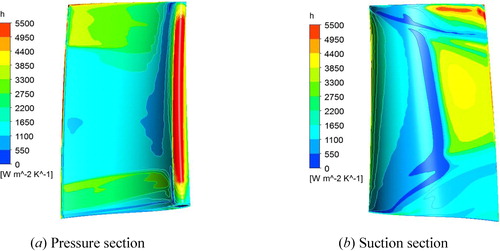
Figure 6. The dimensionless pressure distribution on the blade surface.

3. Scheme design results and discussion

The working environment for the first stage rotor blade is severe. Thus, it is important to design the cooling structure to make the temperature on the blade surface to be lower than the permissible temperature. In the cooling structure design, the thickness of the blade is important. The blade thickness is directly related to the flow passage area and structural strength. The thickness of the blade wall is shown in Figure 7. The thickest areas appear at the leading edge because the film hole will be inserted in this region. At the trailing edge of the pressure section, the thickness is small because the cutback trailing edge will be used. At the root of the blade, the thickness is normally largest while it is small in the tip blade section.

Figure 7. The thickness of the blade wall.

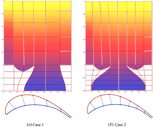
After the thickness design, the blade is divided into several elements. The geometry of the cooling structure will be generated in each element. Two different element designs are shown in Figure 8. In Case 1, the blade is divided into 6 columns and 9 rows. The Case 2 is divided into 8 columns and 10 rows. The flow passage area of each passage is controlled by the red line. The red lines represent the partition walls of the blade. The angle and location of the partition walls decide the flow passage area. The heat transfer and friction factor are linked with the flow passage area directly. It is not enough to calculate the mass flow rate and heat transfer because the flow direction is not defined. In the next step, the attributes for each block are defined. The attributes include the flow direction, the location and size of the film holes, impingement hole, and purge holes.

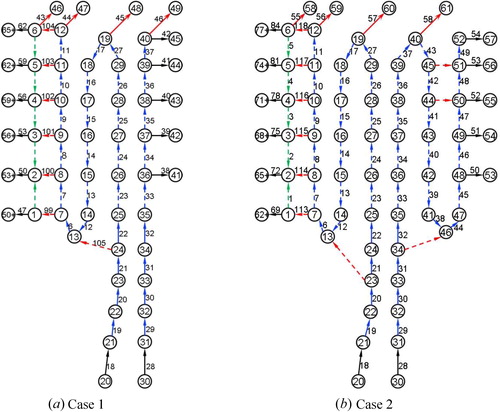
Figure 8. The blocks for different cases.

Figure 9 shows the two different cases according to the different blocks. Concerning Case 1, there are two inlets for the cooling air. The first cooling air inlet is the passage 4 (shown in Figure 8). The cooling air flows through passage 4, passage 3, passage 2, successively. Then, the cooling air impinges onto the passage 1 by the impingement holes which are located between the passage 1 and passage 2. According to the design, 10 impingement holes are located between the passage 1 and passage 2. Usually, the orientation of the impingement holes is normal to the leading edge. The diameter of the impingement hole is 2 mm. Finally, the cooling air leaves the blade through the film hole passage 1. The leading edge is equipped with three rows of staggered cylindrical holes. Each row has 18 0.6 mm cooling holes. The film holes are spread over 90% in the span wise direction. The cooling air of passage 5 will leave the blade from the 90-deg turned trailing edge. Apart from the trailing edge and film hole, part of the cooling air will leave the blade from the tip purge holes. There are four purge holes in the blade tip to protect this region. The diameter of the purge hole is 0.5 mm. Ribs are used in passage 2, passage 3, and passage 4 to enhance the heat transfer coefficient. The height, rib to rib pitch and attack angle of the ribs is 0.2 mm, 10 mm, and 60°, respectively. In passage 1, there are no rib and pin-fin to enhance the heat transfer. At the trailing edge, four rows of pin-fins are used in passage 6. The diameter of the pin-fins is 1.2 mm; each row is equipped with 16 pin-fins. The Case 2 also has two cooling air inlets, but the flow cross section for the different passages is quite different for different blocks. The cooling air which flows into the first cooling air inlet will also flow through passage 4, passage 3, passage 2, respectively. Then, the cooling air impinges into passage 1. Finally, the cooling air leaves the blade by the film holes which are located at passage 1. The flow condition is similar to that in Case 1. The cooling air which flows into passage 5 will flow through passage 5 and passage 6. Finally, the cooling air leaves the blade though the trailing edge. To avoid backflow of the mainstream, a cooling air channel is added at the top blade between passage 6 and passage 7. Ribs are used in passage 2, passage 3, passage 4, passage 5, and passage 6. The arrangements of the pin-fins, film holes, purge holes, and ribs are similar to Case 1.

Figure 9. The flow pipe-network for different cases.

The block which defines the arrangement can be used in the pipe-network computations. The 1-D results calculated from the pipe-network model show that the total amount of cooling air mass is similar for both two cases (Table 2). However, the cooling air in the second cooling air inlet of Case 1 is larger than for Case 2 which might be related to less passages and lower flow resistance of Case 1 compared with the Case 2. Accordingly, the temperature of Case 2 is too high to be acceptable. Temperature distributions in the blade surface are obtained from the pipe-network, as shown in Figure 10. For Case 1, high temperature occurs in the lower-center of the leading edge and the blade tip of the trailing edge. It also found that the suction section has lower temperature. For Case 2, the highest temperature region is observed at the middle pressure surface of the trailing edge. The reason is that the cooling air flow rate is too small to cool the trailing edge.

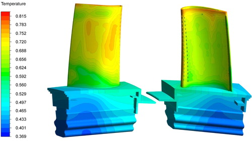
Figure 10. Temperature distributions of the blade surface for different case.

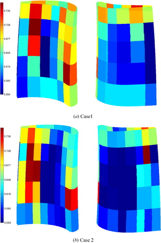
Table 2. The one-dimensional (1-D) results.

	$m_1^{\mathrm{*}}$	$m_2^{\mathrm{*}}$	$m_t^{\mathrm{*}}$	$T_{\mathrm{ave}}^{\mathrm{*}}$	$T_{\max }^{\mathrm{*}}$
Case 1	0.0152	0.0207	0.0359	0.6329	0.7810
Case 2	0.0208	0.0152	0.0360	0.6648	0.9190

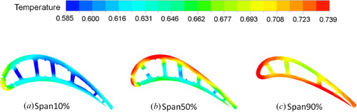
After the pipe-network calculations, the mesh is already generated for the solid domain to calculate the heat conduction. Table 3 shows the 1-D results according to the 3-D heat conduction calculations. The average temperature and the maximum temperature are similar to the pipe-network results. The largest error between the pipe-network and heat conduction simulations is less than 9.3%. The temperature distributions of the blade surfaces are obtained from the 3-D conduction calculation, as shown in Figure 11. It is obvious that the temperature distribution is similar to the pip-network one. A higher temperature region can be observed at the 30–50% spanwise of the blade leading edge, and it is obvious that this high temperature region of Case 1 is larger than that of Case 2. At the middle chord portion of the blade, the temperature distributions of Case 2 are lower than Case 1. Concerning the trailing edge, higher temperature occurs in Case 2, as the cooling air flow is too small to cool the blade. Figure 12 shows the temperature at 10%, 50%, and 90% section, respectively. The high temperature regions at the blade leading and trailing edges also occur and lower temperature distributions can be also observed in Case 2.

Figure 11. Temperature distributions for different cases according to the heat conduction calculations.

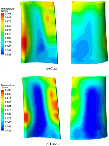
Figure 12. Temperature distributions of different sections according to the heat conduction calculations.

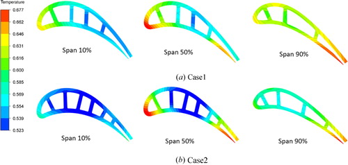
Table 3. The 1-D temperature according to heat conductive.

	$T_{\mathrm{ave}}^{\mathrm{*}}$	$T_{\max }^{\mathrm{*}}$
Case 1	0.601	0.715
Case 2	0.636	0.908

Table 4. Grid independence test for the conjugate calculations.

Mesh number (million)	10	15	23	28	35	40
Average temperature	0.6940	0.6952	0.6738	0.6988	0.6909	0.6903
M2	0.0228	0.0230	0.0226	0.0232	0.0228	0.0228

4. Detailed design results and discussion

According to the pipe-network and the 3-D heat conduction calculation results, the Case 1 shows better performance with limited cooling air flow. Thus, the Case 1 is chosen as the scheme cooling structure. After the scheme design, the geometry is imported into the NX (architectural design software). The pin fins, film holes, and ribs are added in NX. As shown in Figure 13, three rows of film holes, four rows of pin-fins, ribs, and four purge holes are arranged at the blade leading edge, inner tunnels, trailing edge, and blade tip, respectively.

Figure 13. The schematics of the 3-D geometry.

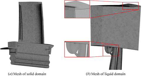
The numerical domain is discretized with an unstructured mesh which is generated by the ICEM (mesh generation software). The prism layer is used to predict the flow and heat transfer in the boundary layers. To balance the prediction accuracy and save computational resources, grid independence tests for the numerical simulations have been carried out (shown in Table 4). It is found that the temperature and mass flow rate are almost constant as the mesh number increases from 35 million to 40 million, and the mesh number 35 million schemes is employed for the numerical simulations.

Figure 14 shows the unstructured grid with prism layers near the fluid wall. The SST turbulence model with g-Req transition model is employed in the 3-D conjugate heat transfer calculations.

Figure 14. Grid of the aero-thermal conjugate calculations.

According to the 3-D conjugate heat transfer calculations, the mass flow rate of the first cooling inlet and second cooling inlet are 0.0161, 0.0228, respectively. The results of the pipe-network are consistent with the 3-D conjugate heat transfer calculations. The maximum error is about 10.86% for the mass flow. The temperature distributions of different sections from the conjugate heat transfer calculations are presented in Figure 15. It is found that a high temperature region occurs on the top of the blade leading edge and pressure section side. For the blade middle part, the temperature of the suction side is higher, which can be related to the flow transition.

Figure 15. Temperature distributions for different sections according to the conjugate heat transfer calculations.

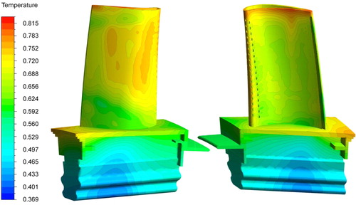
Figure 16 shows the temperature contours of the blade surface. The maximum dimensionless temperature is up to 0.8647 at the blade tip for the pressure section, which is higher than the material permitted temperature. This can be attributed to the leakage flow at the tip clearance which weakens the effect of the purge holes. The temperature requirement cannot be met relying on the internal cooling technology. Hence, a minor revision of the cooling structure is required.

Figure 16. Temperature distributions on the blade surface according to the conjugate heat transfer calculations.

To decrease the high temperature at the blade tip, two film holes are added on the pressure section of the blade tip (shown in Figure 17). The diameter of the film holes is 0.6 mm, and the angle is about 60°.

Figure 17. The 3-D geometry after adjustment.

As shown in Figure 18, the maximum dimensionless temperature is about 0.813, which is lower than the design requirement. The maximum temperature occurs at the leading edge because of the highest heat load. The decreased temperature near the tip of the pressure side can be related to the film cooling. Correspondingly, the leakage flow rate also decreases because of the film holes. The mass flow rate in the first cooling inlet is 0.0168, the mass flow rate in the secondary inlet is 0.0231. There are lower than the requirements.

Figure 18. Temperature distributions on the blade surface after adjustment.

5. Conclusions

In this study, a multilevel cooling structure design system with high robustness, calculation speed, and accuracy for a gas turbine blade was introduced. It is divided into an overall design and detailed design. With this design platform, a complex cooling structure of the first stage rotor blade was designed. The main conclusions from this study are summarized as follows.

1. In this turbine blade cooling structure system, the pipe-network calculations, 3-D heat conduction calculations, and 3-D conjugate heat transfer calculations are combined uniquely, depending on their respective advantages. This process can avoid the blindness with ample and fast scheme design and analysis at the early stage, and then more accurate results and minor revisions will be achieved in the detailed design.

2. Two typical cooling structures were compared and analyzed. The results show that Case 1 has better performance in terms of the average and maximum temperature of the blade outside surface. The temperature deviation between the pipe-network and heat conduction is less than 9.3%.

3. According to the Case 1 pipe-network and the 3-D heat conduction calculations results, a detailed design was completed. The maximum dimensionless temperature of the blade surface is about 0.813 which is lower than required. The mass flow rates for the two cooling inlets are 0.0168 and 0.0231, respectively. These are well below the requirement.

Nomenclature
A	=	heat transfer area, m2
Cf	=	cylinder diameter, mm
Cp	=	specific heat, J/(kg·K)
CFD	=	computational fluid dynamics
h	=	heat transfer coefficient, W/(m2·K)
h*	=	total enthalpy, J
k	=	turbulent kinetic energy, m2/s2
L	=	pipe range, m
mde	=	inlet mass flow, kg/s
p	=	Pressure, Pa
qij	=	mass flow of node
Q	=	heat energy, J
T	=	Temperature, K
Tc	=	static temperature, K
$\overline{T}$	=	total (or stagnation) temperature, K
Twall	=	wall temperature, K
Ua	=	equivalent heat transfer coefficient, W/ (m2·K)
V	=	Velocity, m/s
Greek symbols	=
β	=	yaw angle, °
γ	=	specific heat ratio
δ	=	solid thickness, m
λ	=	thermal conductivity, W/(m·K)
μ	=	dynamic viscosity, kg/(m·s)
μt	=	turbulent viscosity, kg/(m·s)
ρ	=	density of air, kg/m3
Ω	=	rotation speed, rad/s
ω	=	specific dissipation rate
Subscripts	=
in	=	inlet
t	=	total

Additional information

Funding

The authors acknowledge the financial support provided by Natural Science Foundation of China (No. 51706051), China Postdoctoral Science Foundation funded project (No. 2017M620116), Heilongjiang Postdoctoral Fund (No. LBH-Z17066), the General and Special Program of the Postdoctoral Science Foundation of China (No. 2018T110296) and the Fundamental Research Funds for the Central Universities (Grant No. HIT.NSRIF.2019061).

References

- R. S. Bunker, “A review of shaped hole turbine film-cooling technology,” J. Heat Transf., vol. 127, no. 4, pp. 441–453, Apr. 2005. DOI: 10.1115/1.1860562.
- D. G. Bogard and K. A. Thole, “Gas turbine film cooling,” J. Propul. Power, vol. 22, no. 2, pp. 249–269, 2006. DOI: 10.2514/1.18034.
- N. Hay and D. Lampard, “Discharge coefficient of turbine cooling holes: A review,” J. Turbomach., vol. 120, no. 2, pp. 314–319, 1998. DOI: 10.1115/1.2841408.
- J. C. Han, S. Dutta, and S. Ekkad, Gas Turbine Heat Transfer and Cooling Technology. Boca Raton, FL, USA: Taylor & Francis Group, 2012.
- G. J. Korotky and M. E. Taslim, “Rib heat transfer coefficient measurements in a rib-roughened square passage,” Proceedings of the ASME 1996 International Gas Turbine and Aeroengine Congress and Exhibition. Volume 4: Heat Transfer; Electric Power; Industrial and Cogeneration, Birmingham, UK, Jun. 1996. DOI: 10.1115/96-GT-356.
- J. C. Han, Y. M. Zhang, and C. P. Lee, “Augmented heat transfer in square channels with parallel, crossed, and V-shaped angled ribs,” J. Heat Transf., vol. 113, no. 3, pp. 590–596, 1991. DOI: 10.1115/1.2910606.
- Y. Li, H. Deng, G. Xu, and S. Tian, “Heat transfer and pressure drop in a rotating two-pass square channel with different ribs at high rotation numbers,” Proceedings of the ASME Turbo Expo 2015: Turbine Technical Conference and Exposition, ASME Paper GT2015-44019, Montreal, Quebec, Canada, Jun. 2015. DOI: 10.1115/GT2015-44019.
- J. Armstrong and D. Winstanley, “A review of staggered array pin fin heat transfer for turbine cooling applications,” J. Turbomach., vol. 110, no. 1, pp. 94–103, Jan. 1988. DOI: 10.1115/1.3262173.
- D. E. Metzger, C. S. Fan, and S. W. Haley, “Effects of pin shape and array orientation on heat transfer and pressure loss in pin fin arrays,” J. Eng. Gas Turbines Power, vol. 106, no. 1, pp. 252–257, Jan. 1984. DOI: 10.1115/1.3239545.
- L. M. Wright, E. Lee, and J. C. Han, “Effect of rotation on heat transfer in rectangular channels with pin-fins,” J. Thermophys. Heat Transf., vol. 18, no. 2, pp. 263–272, Apr. 2004. DOI: 10.2514/1.4723.
- P. Li and K. Y. Kim, “Multiobjective optimization of staggered elliptical pin-Fin arrays,” Numer. Heat Transf. A: Appl., vol. 53, no. 4, pp. 418–431, 2008. DOI: 10.1080/10407780701632759.
- L. Luo, Y. F. Zhang, C. L. Wang, S. T. Wang, and B. Sundén, “On the heat transfer characteristics of a Lamilloy cooling structure with curvatures with different pin fins configurations,” Int. J. Numer. Methods Heat Fluid Flow, 2020.
- L. Luo, C. L. Wang, L. Wang, B. Sundén, and S. T. Wang, “Heat transfer and friction factor performance in a pin fin wedge duct with different dimple arrangements,” Numer. Heat Transf. A: Appl., vol. 69, no. 2, pp. 209–226, Nov. 2016. DOI: 10.1080/10407782.2015.1052301.
- L. Luo et al., “Surface temperature reduction by using dimples/protrusions in a realistic turbine blade trailing edge,” Numer. Heat Transf. A: Appl., vol. 74, no. 5, pp. 1265–1283, 2018. DOI: 10.1080/10407782.2018.1515333.
- M. E. Taslim and A. Nongsaeng, “Experimental and numerical cross-over jet impingement in an airfoil trailing-edge cooling channel,” J. Turbomach., vol. 133, no. 4, Oct. 2011. DOI: 10.1115/1.4002984.
- P. Martini, A. Schulz, and S. Wittig, “Experimental and numerical investigation of trailing edge film cooling by circular coolant wall jets ejected from a slot with internal rib arrays,” J. Turbomach., vol. 126, no. 2, pp. 229–236, Apr. 2004. DOI: 10.1115/1.1645531.
- J. Wang, J. Liu, L. Wang, B. Sundén, and S. Wang, “Conjugated heat transfer investigation with racetrack-shaped jet hole and double swirling chamber in rotating jet impingement,” Numer. Heat Transf. A: Appl., vol. 73, no. 11, pp. 768–787, 2018. DOI: 10.1080/10407782.2018.1454753.
- K. Singh, R. Das, and B. Kundu, “Approximate analytical method for porous stepped fins with temperature-dependent heat transfer parameters,” J. Thermophys. Heat Transf., vol. 30, no. 3, pp. 661–672, May 2016. DOI: 10.2514/1.T4831.
- R. Das and B. Kundu, “Prediction of heat generation in a porous fin from surface temperature,” J. Thermophys. Heat Transf., vol. 31, no. 4, pp. 781–790, Feb. 2017. DOI: 10.2514/1.T5098.
- W. P. Damerow, J. C. Murtaugh, and F. Burgraf, “Experimental and analytical investigation of the coolant flow characteristics in cooled turbine airfoils,” NASA Technical Paper, NASA-CR-120883, 1972.
- P. L. Meitner, “Computer code for predicting coolant flow and heat transfer in turbomachinery,” NASA Technical Paper 2985, AVSCOM Technical Paper 89-C-008, 1990.
- C. Carcasci and B. Facchini, “A numerical procedure to design internal cooling of gas turbine stator blades,” Rev. Gen. Therm., vol. 35, no. 412, pp. 257–268, 1996. DOI: 10.1016/S0035-3159(96)80018-3.
- G. H. Kumar, R. J. Richard, and P. L. Meitner, “A generalized one dimensional computer code for turbomachinery cooling passage flow calculations,” presented at the 25th Joint Propulsion Conference, AIAA: Monterey, California, USA, Jul. 1989. DOI: 10.2514/6.1989-2574.
- A. Majumdar, J. W. Bailey, P. Schallhorn, and T. Steadman, “A generalized fluid system simulation program to model flow distribution in fluid networks,” presented at the 33rd Joint Propulsion Conference and Exhibit, Sverdrup Technology Report No. 331-201-97-005, AIAA: Cleveland, Ohio, USA, Jul. 1997. DOI: 10.2514/6.1997-3225.
- K. J. Kutz and T. M. Speer, “Simulation of the secondary air system of aero engines,” Proceedings of the ASME 1992 International Gas Turbine and Aeroengine Congress and Exposition. Volume 1: Turbomachinery, ASME: Cologne, Germany, Jun. 1992. DOI: 10.1115/92-GT-068.
- S. S. Talya, A. Chattopadhyay, and J. N. Rajadas, “An integrated multidisciplinary design optimization procedure for cooled gas turbine blades,” presented at the 41st Structures, Structural Dynamics, and Materials Conference and Exhibit, AIAA Paper 2000-1664, Apr. 2000. DOI: 10.2514/6.2000-1664.
- S. S. Talya, A. Chattopadhyay, and J. N. Rajadas, “Multidisciplinary design optimization procedure for improved design of a cooled gas turbine blade,” Eng. Optimiz., vol. 34, no. 2, pp. 175–194, 2002. DOI: 10.1080/03052150210917.
- N. Jelisavcic et al., “Design optimization of networks of cooling passages,” ASME 2005 International Mechanical Engineering Congress and Exposition. Heat Transfer, Part B, Orlando, Florida, USA, Nov. 2005, pp. 399–410. DOI: 10.1115/IMECE2005-79175.
- T. J. Martin and G. S. Dulikravich, “Analysis and multidisciplinary optimization of internal coolant networks in turbine blades,” J. Propul. Power, vol. 18, no. 4, pp. 896–906, 2002. DOI: 10.2514/2.6015.
- K. H. Yu, Z. F. Yue, and J. Wang, “Parametric modeling and multidisciplinary design optimization of 3-d internally cooled turbine blades,” presented at the 7th AIAA Aviation Technology, Integration and Operations Conference, Sep. 2007. AIAA Paper 2007-7719. DOI: 10.2514/6.2007-7719.
- V. K. Kostege, V. A. Halturin, and V. G. Sundurin, Simulation of Multidisciplinary Problems for the Thermostress State of Cooled High Temperature Turbines. AGARD Lecture Series TCP 02/LS198: Math. Models Gas Turbine Engines Their Components, London, UK, 1994.
- H. F. Jen and J. B. Sobanik, “Cooling air flow characteristics in gas turbine components,” J. Eng. Gas Turbine Power, vol. 104, no. 2, pp. 275–280, 1982. DOI: 10.1115/1.3227276.
- G. N. Kumar, R. J. Roelky, and P. L. Meiner, “A generalized one dimensional computer code for turbomachinery cooling passage flow calculations,” presented at the 25th Joint Propulsion Conference, AIAA Paper 89-2574, Reston, VA, USA, Jul. 1989. DOI: 10.2514/6.1989-2574.
- H. K. Versteeg and W. Malalasekera, An Introduction to Computational Fluid Dynamics: The Finite Volume Method. Glasgow, UK: Pearson Education, 2007.
- L. Luo, B. Sundén, and S. T. Wang, “Optimization of the blade profile and cooling structure in a gas turbine stage considering both aerodynamics and heat transfer,” Heat Transf. Res., vol. 46, no. 7, pp. 599–629, 2015. DOI: 10.1615/HeatTransRes.2015012370.
- L. Luo, C. Wang, L. Wang, B. Sundén, and S. T. Wang, “Endwall heat transfer and aerodynamic performance of bowed outlet guide vanes (OGVs) with on- and off-design conditions,” Numer. Heat Transf. A: Appl., vol. 69, no. 4, pp. 352–368, Nov. 2016. DOI: 10.1080/10407782.2015.1081021.
- L. Luo, C. Wang, L. Wang, B. Sundén, and S. T. Wang, “Computational investigation of dimple effects on heat transfer and friction factor in a Lamilloy cooling structure,” J Enhanc. Heat Transf., vol. 22, no. 2, pp. 147–175, 2015. DOI: 10.1615/JEnhHeatTransf.2015013956.
- W.-T. Su, M. Binama, Y. Li, and Y. Zhao, “Study on the method of reducing the pressure fluctuation of hydraulic turbine by optimizing the draft tube pressure distribution,” Renew. Energy, vol. 162, pp. 550–560, Jul. 2020. DOI: 10.1016/j.renene.2020.08.057.
- F. R. Menter, “Two-equation eddy-viscosity turbulence models for engineering applications,” AIAA J., vol. 32, no. 8, pp. 1598–1605, 1994. DOI: 10.2514/3.12149.
- L. D. Hylton, M. S. Milhec, E. R. Turner, D. A. Nealy, and R. E. York, “Analytical and experimental evaluation of the heat transfer distribution over the surface of turbine vanes,” NASA-CR-168015, Cleveland, OH, USA, May 1983.