Generalized UNIFAES derivatives applied to the correlations of the transport equations for fluctuating kinetic energy, helicity and enstrophy in an oscillated laminar flow

Abstract

The original UNIFAES, as any exponential-type scheme, applies to the combined advective and diffusive terms of the viscous fluid transport equations. This work generalizes the scheme by making explicit the first and second derivatives of its interpolating curve, so that it can be applied, alongside classic central differencing schemes, to the statistical correlations of the transport equations of fluctuating kinetic energy, helicity and enstrophy. Tests are performed in a perturbed laminar incompressible Couette flow, obtained with a three-dimensional primitive variables solver using the original UNIFAES, the semi-staggered mesh, the Poisson equation for pressure and the forth order Runge-Kutta time-wise integration. Both the asymptotic tendencies of the correlations at low Reynolds number and the numerical stability of the solver for any Reynolds number are demonstrated with modest meshes.

Keywords:

• Enstrophy
• fluctuating kinetic energy
• generalized UNIFAES
• helicity

Introduction

An important theme on numerical fluid dynamics during the second half of past century, in Finite Difference (FD), Finite Volume (FV), and Finite Elements (FE) methods, was the search for discretization schemes for the advective and diffusive transport equations, represented below for a general transported variable $\mathrm{\Phi }$ on an incompressible velocity field ${\mathcal{U}}_i$: (1) $$\frac{\partial \mathrm{\Phi }}{\partial t}+\frac{\partial {\mathcal{U}}_i\mathrm{\Phi }}{\partial x_i}-\nu \frac{{\partial }^2\mathrm{\Phi }}{\partial x_i\partial x_i}=S$$(1)

Here, $\nu$ is the diffusivity of the transported variable and $S$ is a possible source term. Summation over the three coordinate directions is assumed for each repeated index in a term. The advective term can be written in divergence form $\partial {\mathcal{U}}_i\mathrm{\Phi }/\partial x_i,$ as above, or in equivalent advective form ${\mathcal{U}}_i\partial \mathrm{\Phi }/\partial x_i$.

Research for new discretization methods was motivated by the limitations of the classic schemes for the advective term: the second order schemes Central Differencing in FD and FV, as well as Galerkin in FE, are unstable as the advective term dominates over the diffusive term, whist first order Upwind schemes in FD and FV and Petrov-Galerkin in FE are inaccurate. Within the FV approach, two kinds of schemes emerged and remained in use: 1- schemes which use upwind polynomial interpolations to discretize the advective term, maintaining Central Differencing for the diffusive terms, particularly the Second Order Upwind [1] and QUICK [2], and 2- schemes which use exponential interpolations to discretize the combined advective and diffusive terms, particularly the simple Exponential scheme [3] and UNIFAES [4].

UNIFAES has been applied to linear test cases [4–6], to natural and mixed convection in porous media [5–7], and to incompressible Navier-Stokes equations in primitive variables [8–13], including three dimensional flows [14, 15]. Comparative studies in most of these works have shown UNIFAES to be stable and to present superior accuracy than other second order schemes as the Peclet, Rayleigh or Reynolds numbers increase. The most comprehensive comparative study employed seven FV schemes [11–13] to solve the backward facing step flow with $50\times 30$ meshes and multiples up to $250\times 150.$ Recouring to the most refined mesh, Central Differencing Scheme (CDS) could converge up to Reynolds number 600; QUICK, up to Re = 1,000; and the First Order Upwind, up to Re = 1,200. No convergence was obtained with LOADS. Only three schemes were stable with moderate meshes up to Re = 1,200, which is the experimental limit of physical stability: the simple Exponential, the Second Order Upwind (SOU) and UNIFAES.

The accuracy of the schemes was compared via the root mean square of the errors of the velocity field upon the nodes of the $50\times 30$ mesh; reference values were obtained by Richardson extrapolation on these nodes using the more refined meshes. For the lower Reynolds numbers, all second order schemes present close results; UNIFAES is slightly worse than CDS and QUICK and slightly better than SOU and Exponential. For Re = 400, UNIFAES is the most accurate, closely followed by CDS and QUICK on the most refined meshes, then by SOU and Exponential. The distance of UNIFAES to the other schemes increases with the Reynolds number: for Re = 400, the accuracy of UNIFAES at the most refined mesh is superior to that of the SOU by factor 2.5 and to the Exponential scheme by factor 3.3; for Re = 800, these factors increase to 3.4 and 24, respectively. Furthermore, UNIFAES maintains second order dominated solutions at the higher Reynolds number even at moderate meshes, whereas SOU and Exponential are only asymptotically second order.

Such performance makes UNIFAES the best choice, among the schemes considered, for a FV solver of Navier-Stokes equations for direct numerical modeling of turbulence. Yet, at initial steps, construction of the solver and of the algorithm for post processing the relevant statistics motivated the numerical developments here reported.

These statistics concern the terms of the transport equations of fluctuating kinetic energy, helicity and enstrophy, Equations (43)(43) $$\frac{\partial U_j\overline{u_i{u}_i}/2}{\partial x_j}-\nu \frac{{\partial }^2{\overline{u_{i}u}}_i/2}{\partial x_j\partial x_j}=-\overline{u_i{u}_j}{S}_{ij}\mathrm{ }–\frac{\partial \overline{u_{j}p}}{\partial x_j}-\frac{\partial \overline{u_j{u}_i{u}_i}/2}{\partial x_j}\mathrm{ }-\nu \overline{\frac{\partial u_i}{\partial x_j}\frac{\partial u_i}{\partial x_j}}$$(43) to (46)(46) $$\frac{\partial U_j\overline{w_i{w}_i/2}}{\partial x_j}-\upsilon \frac{{\partial }^2\overline{{w_{i}w}_i}/2}{\partial x_j\partial x_j}=\overline{w_i{s}_{ij}}{W}_j+\overline{w_i{w}_j}{S}_{ij}-\overline{w_i{u}_j}\frac{\partial W_i}{\partial x_j}-\frac{\partial \overline{u_j{w}_i{w}_i/2}}{\partial x_j}\text{-}\mathrm{ }\overline{w_i{w}_j{s}_{ij}}\mathrm{ }-\upsilon \overline{\frac{\partial w_i}{\partial x_j}\frac{\partial w_i}{\partial x_j}}$$(46) . The numerous correlations on these equations involve first and second derivatives of mean and fluctuating variables, which can be evaluated by accurate central differencing schemes since these post processing calculations pose no question of stability. However, it would be elegant using schemes which are coherent with that of the solver, expectedly avoiding further errors upon the solver convergence errors. Furthermore, since the interpolating curve of UNIFAES is accurate for the composed advective and diffusive terms, it is possibly accurate for general derivativatives of transported variables.

However, as already observed, UNIFAES directly computes the combined advective and diffusive terms of the transport equation. Determining the first and second derivatives of the interpolating curve is required neither for the algebraic derivation of the scheme nor for solving Navier-Stokes and simple transport equations; these derivatives would naturally be needed when dealing with complex transport equations, such as this case. The first and second derivatives of the interpolating curve of UNIFAES are made explicit in the next section, generalizing the scheme to any term concerning transported variables.

The interpolating curve of exponential-type schemes is dependent on local instantaneous velocity, and so are its derivatives. Therefore, although the first and second differentials are linear operators, UNIFAES approximation to velocity or vorticity derivatives are non-linear operators, dependent on local instantaneous velocity. This paradox was not noticed with the UNIFAES restrict to the combined advective and diffusive terms because advection is a non-linear term. A linear approximation to UNIFAES derivatives is defined by using the local mean velocity field as the unique referential at each node. Both linear and non-linear forms are tested.

The present choice of transport equations follows a consideration raised by Prof. João Fernando Ata de Oliveira Pantoja (private communication, 1982), in a critique to the $K-\epsilon$ turbulence model. A description of turbulence as a random phenomenon should consider the relevant statistical moments: the first moment, which is the mean velocity; the second moment or variance, well represented by kinetic energy $K={\overline{u_{i}u}}_i/2;$ the third moment, skewness or asymmetry, which the $K-\epsilon$ models lack; and the fourth moment, kurtosis, represented by the energy dissipation rate $(\epsilon )$ in these models. Here, this recommendation is followed by using three scalar products of fluctuating velocity and vorticity. Kinetic energy is maintained; helicity, the scalar product of velocity by vorticity, $\overline{{u_{i}w}_i},$ which can be positive, nil or negative, is taken as representative of skewness; and enstrophy, $\overline{{w_{i}w}_i}/2,$ known early as “squared vorticity” [16], represents kurtosis.

The concept of helicity was formulated around 1960, with fruitful applications in magneto hydrodynamics and meteorology. Recalling Moreau’s theorem for inviscid barotropic flows under conservative body forces, which states the conservation of the total helicity within a closed surface that moves with the fluid without penetration of vorticity, Moffatt and Tsinober [17] declare this conservation property to give helicity “a status comparable to energy in the dynamics of ideal fluids”, and wonder about a “possible relation between helicity and vortex breakdown”. Authors of more recent texts in physics fluid mechanics literature report numerical simulations that do relate helicity oscillations to the turbulence cascade [18–20, to name a few]. However, to the present author’s knowledge, helicity is not yet used in engineering turbulence models.

The physical mechanism for turbulent energy cascade is vortex stretching, i.e. vortex tubes being elongated in a varying velocity field, causing the vortex tube to become thinner, with increased rotation to maintain the angular momentum. Therefore, turbulent stretching involves simultaneous collinear acceleration of velocity and vorticity; thus, is related to fluctuations of the scalar product velocity-vorticity, i.e. fluctuating helicity.

Due to being at its initial stages, this work is restricted to mono-processing computer, whose limitations in memory and velocity prevent realistic turbulence measurements and impose a short numerical domain. Using laminar flow cases is necessary for verifying the asymptotic tendencies of the solver and the statistics processor, because turbulent flows introduce sampling errors [21, 22]. The short numerical domain puts strong limitations to representativity of the physical results. For those reasons, this work must be appreciated solely in terms of numerical developments concerning the generalized UNIFAES and the convergence of the correlations of the transport equations.

Unbalances or residuals of the transport equations are the most relevant error indexes regarding the correlations. Convergence of solutions is analyzed by mesh refinement, using the Generalized UNIFAES derivatives, the Second Order Central Differencing and the Fourth Order Central Differencing comparatively. Independent accuracy testing for each discretization scheme is provided by comparing alternative algebraic forms for some terms.

Generalized UNIFAES scheme

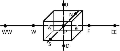
For simplicity, this work is restricted to regularly spaced Cartesian meshes, although UNIFAES admits irregularly spaced meshes without loss of second order convergence, provided adequate refinement strategy is used [6, 7]. The traditional FV geographical compass notation is adopted for the nodes around central node P, as indicated in Figure (1)(1) $$\frac{\partial \mathrm{\Phi }}{\partial t}+\frac{\partial {\mathcal{U}}_i\mathrm{\Phi }}{\partial x_i}-\nu \frac{{\partial }^2\mathrm{\Phi }}{\partial x_i\partial x_i}=S$$(1) .

UNIFAES belongs to a class of schemes developed in FD, FV and FE approaches, whose interpolating curve is obtained as exact solutions of the one-dimensional linear equation: (2) $$\mathcal{U}\frac{d\mathrm{\Phi }}{dx}-\nu \frac{d^2\mathrm{\Phi }}{d{x}^2}=K$$(2)

Equation(2) $$\mathcal{U}\frac{d\mathrm{\Phi }}{dx}-\nu \frac{d^2\mathrm{\Phi }}{d{x}^2}=K$$(2) (2(2) $$\mathcal{U}\frac{d\mathrm{\Phi }}{dx}-\nu \frac{d^2\mathrm{\Phi }}{d{x}^2}=K$$(2) )(2) $$\mathcal{U}\frac{d\mathrm{\Phi }}{dx}-\nu \frac{d^2\mathrm{\Phi }}{d{x}^2}=K$$(2) approximates the transport equation (1)(1) $$\frac{\partial \mathrm{\Phi }}{\partial t}+\frac{\partial {\mathcal{U}}_i\mathrm{\Phi }}{\partial x_i}-\nu \frac{{\partial }^2\mathrm{\Phi }}{\partial x_i\partial x_i}=S$$(1) by assuming the velocity component $\mathcal{U}\mathcal{ }$ in direction $x$ to be locally constant, as well as the term $K,$ which represents the other terms of the equation (1)(1) $$\frac{\partial \mathrm{\Phi }}{\partial t}+\frac{\partial {\mathcal{U}}_i\mathrm{\Phi }}{\partial x_i}-\nu \frac{{\partial }^2\mathrm{\Phi }}{\partial x_i\partial x_i}=S$$(1) , namely cross flow transport, source and transient terms. Thus, this class of schemes could be described as “locally analytic schemes”, an expression adopted for a specific member of the class; here these schemes are called Exponential-type schemes since the function appears when solving the generating equation (2)(2) $$\mathcal{U}\frac{d\mathrm{\Phi }}{dx}-\nu \frac{d^2\mathrm{\Phi }}{d{x}^2}=K$$(2) to obtain the interpolation curve (3)(3) $$\mathrm{\Phi }=C_1+C_2\hspace{0.17em}\exp \hspace{0.17em}\left(\frac{\mathcal{U}.x}{\nu }\right)+\frac{K}{\mathcal{U}}x$$(3) , and in the subsequent algebra: (3) $$\mathrm{\Phi }=C_1+C_2\hspace{0.17em}\exp \hspace{0.17em}\left(\frac{\mathcal{U}.x}{\nu }\right)+\frac{K}{\mathcal{U}}x$$(3)

UNIFAES is the acronym for Unified Finite Approaches Exponential-type Scheme; it is a FV exponential-type scheme completed by recourse to the FD exponential-type scheme due to Allen and Southwell [23]. This scheme, historically the first, is presented initially, followed by general FV exponential-type schemes, leading immediately to the restrict form of UNIFAES; finally, the generalization to first and second derivatives is presented.

Allen and Southwell FD scheme

In Allen and Southwell scheme, the interpolating curve (3)(3) $$\mathrm{\Phi }=C_1+C_2\hspace{0.17em}\exp \hspace{0.17em}\left(\frac{\mathcal{U}.x}{\nu }\right)+\frac{K}{\mathcal{U}}x$$(3) is used to compute the combined advective and diffusive net flux in advective form at node P, ${\mathcal{U}}_P{\left(\partial \mathrm{\Phi }/\partial x\right)}_P-\nu {\left({\partial }^2\mathrm{\Phi }/\partial x^2\right)}_P,$ which is precisely $K_P,$ according to generating equation (2)(2) $$\mathcal{U}\frac{d\mathrm{\Phi }}{dx}-\nu \frac{d^2\mathrm{\Phi }}{d{x}^2}=K$$(2) . The interpolating curve (3)(3) $$\mathrm{\Phi }=C_1+C_2\hspace{0.17em}\exp \hspace{0.17em}\left(\frac{\mathcal{U}.x}{\nu }\right)+\frac{K}{\mathcal{U}}x$$(3) , with unknowns $C_1,$ $C_2$ and $K_P/{\mathcal{U}}_P,$ is fit to the nodes W, P and E (Figure 1), forming a system that can be solved for $K_P$ in terms of cell Peclet number $p_P={\mathcal{U}}_P\Delta x/\upsilon .$ It results in: (4) $$K_P=\left({\mathrm{\Phi }}_P-{\mathrm{\Phi }}_E\right)\frac{\pi \left(p_P\right)}{\Delta x^2}+\left({\mathrm{\Phi }}_P-{\mathrm{\Phi }}_W\right)\frac{\pi \left({-p}_P\right)}{\Delta x^2}$$(4) (5) $$\pi \left(p_P\right)=\frac{p_P}{\exp \left(p_P\right)-1}$$(5)

Figure 1. Control volume and coordinate notation in Finite Volume method.

FV exponential-type schemes

The FV approach proceeds by integrating the divergence form transport equation on the control volume of Figure (1)(1) $$\frac{\partial \mathrm{\Phi }}{\partial t}+\frac{\partial {\mathcal{U}}_i\mathrm{\Phi }}{\partial x_i}-\nu \frac{{\partial }^2\mathrm{\Phi }}{\partial x_i\partial x_i}=S$$(1) , using the divergence theorem. The FV analogue of the net flux $\partial J_1/\partial x_1$ is: $$\frac{\partial J_1}{\partial x_1}\cong \frac{J_e-J_w}{\Delta x_1}=\frac{1}{\Delta x_1\Delta x_2\Delta x_3}{\int }_{{x3}_d}^{{x3}_u}{\int }_{{x2}_s}^{x{2}_n}{\int }_{{x1}_w}^{{x1}_e}\left(\frac{\partial \mathcal{U}\mathrm{\Phi }}{\partial x_1}-\upsilon \frac{{\partial }^2\mathrm{\Phi }}{\partial {x_1}^2}\right)d{x}_{1}d{x}_{2}d{x}_3\cong$$ (6) $$\cong \frac{1}{\Delta x_1}\left[{\mathcal{U}}_e{\mathrm{\Phi }}_{\mathrm{e}}-\upsilon {\frac{\partial \mathrm{\Phi }}{\partial x_1}}_e-{\mathcal{U}}_w{\mathrm{\Phi }}_{\mathrm{w}}+\upsilon {\frac{\partial \mathrm{\Phi }}{\partial x_1}}_w\right]$$(6)

Division by cell volume is used above to restore the physical dimension of the original equation.

The FV Exponential-type schemes employ the interpolating curve (3)(3) $$\mathrm{\Phi }=C_1+C_2\hspace{0.17em}\exp \hspace{0.17em}\left(\frac{\mathcal{U}.x}{\nu }\right)+\frac{K}{\mathcal{U}}x$$(3) to determine the flux through cell face e, for instance, using reference properties at such face. Fitting curve (3)(3) $$\mathrm{\Phi }=C_1+C_2\hspace{0.17em}\exp \hspace{0.17em}\left(\frac{\mathcal{U}.x}{\nu }\right)+\frac{K}{\mathcal{U}}x$$(3) to the nodes P and E, with origin at node P, leads to: (7) $$C_2=\frac{{\mathrm{\Phi }}_{\mathrm{E}}-{\mathrm{\Phi }}_{\mathrm{P}}-\frac{K_e}{u_e}\Delta x}{\exp \left(\frac{{\mathcal{U}}_{\mathrm{e}}\Delta x}{\nu }\right)-1}$$(7) (8) $$C_1={{\mathrm{\Phi }}_{\mathrm{P}}-C}_2$$(8)

Deriving $\mathrm{\Phi }(x)$ from Equation (3)(3) $$\mathrm{\Phi }=C_1+C_2\hspace{0.17em}\exp \hspace{0.17em}\left(\frac{\mathcal{U}.x}{\nu }\right)+\frac{K}{\mathcal{U}}x$$(3) : (9) $$\frac{d\mathrm{\Phi }}{dx}=C_2\frac{\mathcal{U}}{\nu }\exp \hspace{0.17em}\left(\frac{\mathcal{U}.x}{\nu }\right)+\frac{K}{\mathcal{U}}$$(9)

Profile (3)(3) $$\mathrm{\Phi }=C_1+C_2\hspace{0.17em}\exp \hspace{0.17em}\left(\frac{\mathcal{U}.x}{\nu }\right)+\frac{K}{\mathcal{U}}x$$(3) and its derivative (9)(9) $$\frac{d\mathrm{\Phi }}{dx}=C_2\frac{\mathcal{U}}{\nu }\exp \hspace{0.17em}\left(\frac{\mathcal{U}.x}{\nu }\right)+\frac{K}{\mathcal{U}}$$(9) are then employed to compute the combined advective and diffusive flux, expressed at cell face e in terms of the cell face Peclet number $p_e={\mathcal{U}}_e\Delta x_1/\nu$ as: (10) $$J_e={\mathcal{U}}_e{\mathrm{\Phi }}_{\mathrm{e}}-\nu {\frac{\partial \mathrm{\Phi }}{\partial x}}_e={\mathrm{ }{\mathcal{U}}_{e}C}_1+K\left(x_e-\frac{\nu }{{\mathcal{U}}_e}\right)$$(10)

Notice the canceling of terms $C_2\hspace{0.17em}\exp \hspace{0.17em}\left(\mathcal{U}.x/\nu \right)$ in the combined flux $J_e.$ Substituting ${ C}_1$ from Equations (7)(7) $$C_2=\frac{{\mathrm{\Phi }}_{\mathrm{E}}-{\mathrm{\Phi }}_{\mathrm{P}}-\frac{K_e}{u_e}\Delta x}{\exp \left(\frac{{\mathcal{U}}_{\mathrm{e}}\Delta x}{\nu }\right)-1}$$(7) and (8)(8) $$C_1={{\mathrm{\Phi }}_{\mathrm{P}}-C}_2$$(8) into (10)(10) $$J_e={\mathcal{U}}_e{\mathrm{\Phi }}_{\mathrm{e}}-\nu {\frac{\partial \mathrm{\Phi }}{\partial x}}_e={\mathrm{ }{\mathcal{U}}_{e}C}_1+K\left(x_e-\frac{\nu }{{\mathcal{U}}_e}\right)$$(10) leads to: (11) $$J_e=\left({\mathrm{\Phi }}_P-{\mathrm{\Phi }}_E\right)\nu \frac{\pi \left(p_e\right)}{\Delta x_1}+K_e\left[\frac{\pi \left(p_e\right)-1}{p_e}+\frac{1}{2}\right]+{\mathcal{U}}_e{\mathrm{\Phi }}_P$$(11)

Function $\pi \left(p_e\right)$ is computed according to Equation (5)(5) $$\pi \left(p_P\right)=\frac{p_P}{\exp \left(p_P\right)-1}$$(5) . Proceeding analogously for the west side and substituting into (5)(5) $$\pi \left(p_P\right)=\frac{p_P}{\exp \left(p_P\right)-1}$$(5) , the combined advective-diffusive net flux through east and west faces is: (12) $$\frac{J_e-J_w}{\Delta x_1}\cong \frac{1}{\Delta x_1}\left[\nu \frac{\pi \left(p_e\right)}{\Delta x_1}\left({\mathrm{\Phi }}_P-{\mathrm{\Phi }}_E\right)+\nu \frac{\pi \left(p_w\right)}{\Delta x_1}\left({\mathrm{\Phi }}_P-{\mathrm{\Phi }}_W\right)+\mathrm{\Psi }+\left({\mathcal{U}}_e-{\mathcal{U}}_w\right){\mathrm{\Phi }}_P\right]$$(12) (13) $$\mathrm{\Psi }=K_e\mathrm{\chi }\left(p_e\right)-K_w\mathrm{\chi }\left(p_w\right)$$(13) (14) $$\chi \left(p_{e/w}\right)=\frac{\pi \left(p_{e/w}\right)-1}{p_{e/w}}+\frac{1}{2}$$(14)

Term $\left({\mathcal{U}}_e-{\mathcal{U}}_w\right){\Phi }_P/\Delta x_1$ of Equation (12)(12) $$\frac{J_e-J_w}{\Delta x_1}\cong \frac{1}{\Delta x_1}\left[\nu \frac{\pi \left(p_e\right)}{\Delta x_1}\left({\mathrm{\Phi }}_P-{\mathrm{\Phi }}_E\right)+\nu \frac{\pi \left(p_w\right)}{\Delta x_1}\left({\mathrm{\Phi }}_P-{\mathrm{\Phi }}_W\right)+\mathrm{\Psi }+\left({\mathcal{U}}_e-{\mathcal{U}}_w\right){\mathrm{\Phi }}_P\right]$$(12) and its analogues for the other directions vanish due to continuity.

Exponential-type schemes differ according to the treatment of the source terms $K.$ Losing the realism of the interpolation, $K$ is neglected in the simple FV Exponential scheme [3]. Like Allen and Southwell’s, the FV Exponential shows great stability but poor accuracy, resembling the First Order Upwind scheme as the Peclet number increases.

The FV exponential-type schemes which consider the source terms $K$ show much improved accuracy, when stable. The Locally Analytic Differencing Scheme, LOADS [24, 25], estimates $K$ by computing all remaining terms of the complete equation (1)(1) $$\frac{\partial \mathrm{\Phi }}{\partial t}+\frac{\partial {\mathcal{U}}_i\mathrm{\Phi }}{\partial x_i}-\nu \frac{{\partial }^2\mathrm{\Phi }}{\partial x_i\partial x_i}=S$$(1) not considered in (2)(2) $$\mathcal{U}\frac{d\mathrm{\Phi }}{dx}-\nu \frac{d^2\mathrm{\Phi }}{d{x}^2}=K$$(2) , such as cross flow, source terms etc. The Flux-Spline scheme [26–28] iteratively obtains the values of $K$ in the whole field so that the interpolating curves achieve flux continuity. Both approaches turn the flux in a certain direction dependent on information from other directions, in very complex fashions.

Restrict UNIFAES scheme

UNIFAES determines $K$ for Equation(13) $$\mathrm{\Psi }=K_e\mathrm{\chi }\left(p_e\right)-K_w\mathrm{\chi }\left(p_w\right)$$(13) (13(13) $$\mathrm{\Psi }=K_e\mathrm{\chi }\left(p_e\right)-K_w\mathrm{\chi }\left(p_w\right)$$(13) )(13) $$\mathrm{\Psi }=K_e\mathrm{\chi }\left(p_e\right)-K_w\mathrm{\chi }\left(p_w\right)$$(13) by recourse to the Allen and Southwell FD scheme, Equations(4) $$K_P=\left({\mathrm{\Phi }}_P-{\mathrm{\Phi }}_E\right)\frac{\pi \left(p_P\right)}{\Delta x^2}+\left({\mathrm{\Phi }}_P-{\mathrm{\Phi }}_W\right)\frac{\pi \left({-p}_P\right)}{\Delta x^2}$$(4) (4(4) $$K_P=\left({\mathrm{\Phi }}_P-{\mathrm{\Phi }}_E\right)\frac{\pi \left(p_P\right)}{\Delta x^2}+\left({\mathrm{\Phi }}_P-{\mathrm{\Phi }}_W\right)\frac{\pi \left({-p}_P\right)}{\Delta x^2}$$(4) )(4) $$K_P=\left({\mathrm{\Phi }}_P-{\mathrm{\Phi }}_E\right)\frac{\pi \left(p_P\right)}{\Delta x^2}+\left({\mathrm{\Phi }}_P-{\mathrm{\Phi }}_W\right)\frac{\pi \left({-p}_P\right)}{\Delta x^2}$$(4) and (5)(5) $$\pi \left(p_P\right)=\frac{p_P}{\exp \left(p_P\right)-1}$$(5) . The source term $K_e,$ for instance, is generally interpolated from Allen and Southwell estimates of $K_P$ and $K_E;$ if node E is located at a wall, $K_e$ is obtained by extrapolation from $K_P$ and $K_W.$ Since $K_E$ requires the values of ${\Phi }_P, {\Phi }_E$ and ${\Phi }_{EE},$ and $K_W$ requires those of ${\Phi }_P, { \Phi }_W$ and ${\Phi }_{WW},$ the cell stencil generally involves five nodes in each direction. Thus, although the generating equation source term $K$ may represent cross flow, transient, and other terms, when the generating Equation (2)(2) $$\mathcal{U}\frac{d\mathrm{\Phi }}{dx}-\nu \frac{d^2\mathrm{\Phi }}{d{x}^2}=K$$(2) is compared with the full transport Equation (1)(1) $$\frac{\partial \mathrm{\Phi }}{\partial t}+\frac{\partial {\mathcal{U}}_i\mathrm{\Phi }}{\partial x_i}-\nu \frac{{\partial }^2\mathrm{\Phi }}{\partial x_i\partial x_i}=S$$(1) , computation of terms $K$ by Allen and Southwell’s approach turns the UNIFAES representation of the net flux in a specific direction dependent only on data in such direction.

Generalized UNIFAES scheme

The FV analogues of the first and second derivatives in direction $x_1,$ for instance, are obtained by integration on the cell volume by using the divergence theorem. Thus, FV schemes are representative of mean derivatives within the control volume rather than of derivatives at the central node: (15) $$\frac{1}{{\Delta \mathrm{x}}_1}{\int }_{{x1}_w}^{{x1}_e}\frac{\partial \mathrm{\Phi }}{\partial x_1}d{\mathrm{x}}_1=\mathrm{ }\frac{{\mathrm{\Phi }}_{\mathrm{e}}-{\mathrm{\Phi }}_{\mathrm{w}}}{{\Delta \mathrm{x}}_1}\mathrm{ }$$(15) (16) $$\frac{1}{{\Delta \mathrm{x}}_1}{\int }_{{x1}_w}^{{x1}_e}\frac{{\partial }^2\mathrm{\Phi }}{\partial {x_1}^2}d{x}_1=\left({\frac{\partial \mathrm{\Phi }}{\partial x_1}}_e-{\frac{\partial \mathrm{\Phi }}{\partial x_1}}_w\right)\frac{1}{{\Delta \mathrm{x}}_1}$$(16)

The UNIFAES first derivative is produced as follows. From the interpolating curve (3)(3) $$\mathrm{\Phi }=C_1+C_2\hspace{0.17em}\exp \hspace{0.17em}\left(\frac{\mathcal{U}.x}{\nu }\right)+\frac{K}{\mathcal{U}}x$$(3) , by using constants (7)(7) $$C_2=\frac{{\mathrm{\Phi }}_{\mathrm{E}}-{\mathrm{\Phi }}_{\mathrm{P}}-\frac{K_e}{u_e}\Delta x}{\exp \left(\frac{{\mathcal{U}}_{\mathrm{e}}\Delta x}{\nu }\right)-1}$$(7) and (8), one obtains for the cell face e: (17) $${\text{ Φ}}_{\mathrm{e}}={\mathrm{\Phi }}_{\mathrm{P}}+\frac{{\mathrm{\Phi }}_{\mathrm{E}}-{\mathrm{\Phi }}_{\mathrm{P}}}{\exp \left(p_{\mathrm{e}}/2\right)+1}+\frac{K_e}{\upsilon }\frac{\exp \left(p_{\mathrm{e}}/2\right)-1}{2p_{\mathrm{e}}\left(\exp \left(p_{\mathrm{e}}/2\right)+1\right)}$$(17)

Proceeding analogously for the west side and substituting in (15)(15) $$\frac{1}{{\Delta \mathrm{x}}_1}{\int }_{{x1}_w}^{{x1}_e}\frac{\partial \mathrm{\Phi }}{\partial x_1}d{\mathrm{x}}_1=\mathrm{ }\frac{{\mathrm{\Phi }}_{\mathrm{e}}-{\mathrm{\Phi }}_{\mathrm{w}}}{{\Delta \mathrm{x}}_1}\mathrm{ }$$(15) , one obtains UNIFAES first derivative: (18) $$\frac{{\mathrm{\Phi }}_{\mathrm{e}}-{\mathrm{\Phi }}_{\mathrm{w}}}{{\Delta \mathrm{x}}_1}=\frac{\left({\mathrm{\Phi }}_{\mathrm{E}}-{\mathrm{\Phi }}_{\mathrm{P}}\right)\mathrm{\Theta }\left(p_e\right)\text{-}\mathrm{ }\left({\mathrm{\Phi }}_{\mathrm{W}}-{\mathrm{\Phi }}_{\mathrm{P}}\right)\mathrm{\Theta }\left({-p}_w\right)}{{\Delta \mathrm{x}}_1}+\frac{K_e}{\upsilon }\Delta x.\mathrm{\Omega }\left(p_e\right)-\frac{K_w}{\upsilon }\Delta x.\mathrm{\Omega }\left(-p_w\right)$$(18) (19) $$\mathrm{\Theta }\left(p\right)=\frac{1}{\exp \left(p/2\right)+1}$$(19) (20) $$\mathrm{\Omega }\left(p\right)=\frac{\exp \left(p/2\right)-1}{2p\left(\exp \left(p/2\right)+1\right)}=\frac{\mathrm{\Theta }\left(p\right)}{4\pi \left(p/2\right)}$$(20)

The advective term can be reproduced in divergence form as $\left({\mathcal{U}}_e{\mathrm{\Phi }}_{\mathrm{e}}-{{\mathcal{U}}_w\mathrm{\Phi }}_{\mathrm{w}}\right)/{\Delta \mathrm{x}}_1,$ employing Equation (17)(17) $${\text{ Φ}}_{\mathrm{e}}={\mathrm{\Phi }}_{\mathrm{P}}+\frac{{\mathrm{\Phi }}_{\mathrm{E}}-{\mathrm{\Phi }}_{\mathrm{P}}}{\exp \left(p_{\mathrm{e}}/2\right)+1}+\frac{K_e}{\upsilon }\frac{\exp \left(p_{\mathrm{e}}/2\right)-1}{2p_{\mathrm{e}}\left(\exp \left(p_{\mathrm{e}}/2\right)+1\right)}$$(17) and its analogue for ${\mathrm{\Phi }}_{\mathrm{w}},$ and canceling $\left({\mathcal{U}}_e-{\mathcal{U}}_w\right){\Phi }_P/\Delta x_1$ alongside its analogues for other directions due to continuity. Also, emphasizing the generality of the definition above, the advective term can be computed in advective form ${\mathcal{U}}_P\left({\mathrm{\Phi }}_{\mathrm{e}}-{\mathrm{\Phi }}_{\mathrm{w}}\right)/{\Delta \mathrm{x}}_1,$ employing Equation (18)(18) $$\frac{{\mathrm{\Phi }}_{\mathrm{e}}-{\mathrm{\Phi }}_{\mathrm{w}}}{{\Delta \mathrm{x}}_1}=\frac{\left({\mathrm{\Phi }}_{\mathrm{E}}-{\mathrm{\Phi }}_{\mathrm{P}}\right)\mathrm{\Theta }\left(p_e\right)\text{-}\mathrm{ }\left({\mathrm{\Phi }}_{\mathrm{W}}-{\mathrm{\Phi }}_{\mathrm{P}}\right)\mathrm{\Theta }\left({-p}_w\right)}{{\Delta \mathrm{x}}_1}+\frac{K_e}{\upsilon }\Delta x.\mathrm{\Omega }\left(p_e\right)-\frac{K_w}{\upsilon }\Delta x.\mathrm{\Omega }\left(-p_w\right)$$(18) , despite the divergence form of UNIFAES.

Using Equation (9)(9) $$\frac{d\mathrm{\Phi }}{dx}=C_2\frac{\mathcal{U}}{\nu }\exp \hspace{0.17em}\left(\frac{\mathcal{U}.x}{\nu }\right)+\frac{K}{\mathcal{U}}$$(9) with constants (7)(7) $$C_2=\frac{{\mathrm{\Phi }}_{\mathrm{E}}-{\mathrm{\Phi }}_{\mathrm{P}}-\frac{K_e}{u_e}\Delta x}{\exp \left(\frac{{\mathcal{U}}_{\mathrm{e}}\Delta x}{\nu }\right)-1}$$(7) and (8), one obtains for the cell face e: (21) $${\frac{\partial \mathrm{\Phi }}{\partial \mathrm{x}}}_{\mathrm{e}}=\frac{{\mathrm{\Phi }}_{\mathrm{E}}-{\mathrm{\Phi }}_{\mathrm{P}}+\frac{K_e}{u_e}\Delta x}{\exp \left(p_e\right)-1}.\frac{p_e}{\Delta x}.\exp \left(\frac{p_e}{2}\right)+\frac{K_e}{u_e}$$(21)

By proceeding analogously for face w and substituting into (16)(16) $$\frac{1}{{\Delta \mathrm{x}}_1}{\int }_{{x1}_w}^{{x1}_e}\frac{{\partial }^2\mathrm{\Phi }}{\partial {x_1}^2}d{x}_1=\left({\frac{\partial \mathrm{\Phi }}{\partial x_1}}_e-{\frac{\partial \mathrm{\Phi }}{\partial x_1}}_w\right)\frac{1}{{\Delta \mathrm{x}}_1}$$(16) one obtains UNIFAES second derivative: (22) $$\left({\frac{\partial \mathrm{\Phi }}{\partial \mathrm{x}}}_{\mathrm{e}}-{\frac{\partial \mathrm{\Phi }}{\partial \mathrm{x}}}_{\mathrm{w}}\right)\frac{1}{\Delta \mathrm{x}}=\frac{{\mathrm{\Phi }}_{\mathrm{E}}-{\mathrm{\Phi }}_{\mathrm{P}}}{{\Delta \mathrm{x}}^2}\lambda \left(p_e\right)+\frac{{\mathrm{\Phi }}_{\mathrm{W}}-{\mathrm{\Phi }}_{\mathrm{P}}}{{\Delta \mathrm{x}}^2}\lambda \left(-p_w\right)+\frac{K_e}{\upsilon }.\mathrm{{\rm Y}}\left(p_e\right)+\frac{K_w}{\upsilon }.\mathrm{{\rm Y}}\left({-p}_w\right)$$(22) (23) $$\lambda \left(p\right)=\frac{p.\exp \left(\frac{p}{2}\right)}{\exp \left(p\right)-1}=\mathrm{\pi }\left(p\right)\hspace{0.17em}\exp \hspace{0.17em}\left(\frac{p}{2}\right)$$(23) (24) $$\mathrm{{\rm Y}}\left(p\right)=\frac{1\text{-}\mathrm{\pi }\left(p\right)\hspace{0.17em}\exp \hspace{0.17em}\left(\frac{p}{2}\right)}{p}$$(24)

Notice the appearance of exponentials of half cell Peclet numbers, which did not appear in the expression of the combined advective and diffusive flux due to canceling an exponential term. All functions with exponentials in Equations (5)(5) $$\pi \left(p_P\right)=\frac{p_P}{\exp \left(p_P\right)-1}$$(5) , (14)(14) $$\chi \left(p_{e/w}\right)=\frac{\pi \left(p_{e/w}\right)-1}{p_{e/w}}+\frac{1}{2}$$(14) , (19)(19) $$\mathrm{\Theta }\left(p\right)=\frac{1}{\exp \left(p/2\right)+1}$$(19) , (20)(20) $$\mathrm{\Omega }\left(p\right)=\frac{\exp \left(p/2\right)-1}{2p\left(\exp \left(p/2\right)+1\right)}=\frac{\mathrm{\Theta }\left(p\right)}{4\pi \left(p/2\right)}$$(20) , (23)(23) $$\lambda \left(p\right)=\frac{p.\exp \left(\frac{p}{2}\right)}{\exp \left(p\right)-1}=\mathrm{\pi }\left(p\right)\hspace{0.17em}\exp \hspace{0.17em}\left(\frac{p}{2}\right)$$(23) and (24)(24) $$\mathrm{{\rm Y}}\left(p\right)=\frac{1\text{-}\mathrm{\pi }\left(p\right)\hspace{0.17em}\exp \hspace{0.17em}\left(\frac{p}{2}\right)}{p}$$(24) require trivial asymptotic approximations for cell Peclet numbers exceeding the computational limits for the arguments of exponentials. Functions $\pi ,\mathrm{ }\chi ,$ and $\mathrm{{\rm Y}}$ also require asymptotic approximations in a neighborhood of the origin, where they are formally singular.

Depending on local instantaneous velocities, the generalized UNIFAES are non-linear difference operators representing linear differential operators. As one of its consequences, the mean of a velocity derivative using instantaneous velocities is not the mean derivative, differently from usual scheme.

The UNIFAES approximation to derivative of velocity ${U_i+u}_i$ in the direction j, computed by analogy with variable $\mathrm{\Phi }$ in Equation (18)(18) $$\frac{{\mathrm{\Phi }}_{\mathrm{e}}-{\mathrm{\Phi }}_{\mathrm{w}}}{{\Delta \mathrm{x}}_1}=\frac{\left({\mathrm{\Phi }}_{\mathrm{E}}-{\mathrm{\Phi }}_{\mathrm{P}}\right)\mathrm{\Theta }\left(p_e\right)\text{-}\mathrm{ }\left({\mathrm{\Phi }}_{\mathrm{W}}-{\mathrm{\Phi }}_{\mathrm{P}}\right)\mathrm{\Theta }\left({-p}_w\right)}{{\Delta \mathrm{x}}_1}+\frac{K_e}{\upsilon }\Delta x.\mathrm{\Omega }\left(p_e\right)-\frac{K_w}{\upsilon }\Delta x.\mathrm{\Omega }\left(-p_w\right)$$(18) , is expressed below by a tilt upon the differential symbol, and the reference velocity used in the cell Peclet number is indicated as subscript of the derivation. To follow with rigor the scheme used in the Navier-Stokes solver, determining the UNIFAES derivative of the fluctuating component requires computing derivatives of instantaneous velocities at instantaneous conditions and computing derivatives of mean velocities at mean conditions, as follows: (25) $$\widetilde{\frac{\partial u_i}{\partial x_j}}={\tilde{\frac{\partial \left({U_i+u}_i\right)}{\partial x_j}}}_{{U_j+u}_j}\text{-}\mathrm{ }{\widetilde{\frac{\partial U_i}{\partial x_j}}}_{{\mathrm{ }U}_j}$$(25)

No summation on $j-$ direction is implied here. This procedure differs from applying UNIFAES derivation directly to the fluctuating velocity components, as expressed in the left member of Equation (26)(26) $${\mathrm{ }\widetilde{\frac{\partial u_i}{\partial x_j}}}_{{{\mathrm{ }U}_j+u}_j}=\mathrm{ }{\tilde{\frac{\partial \left({U_i+u}_i\right)}{\partial x_j}}}_{{U_j+u}_j}\text{-}\mathrm{ }{\widetilde{\frac{\partial U_i}{\partial x_j}}}_{{{\mathrm{ }U}_j+u}_j}$$(26) , which would be equivalent to the right member: (26) $${\mathrm{ }\widetilde{\frac{\partial u_i}{\partial x_j}}}_{{{\mathrm{ }U}_j+u}_j}=\mathrm{ }{\tilde{\frac{\partial \left({U_i+u}_i\right)}{\partial x_j}}}_{{U_j+u}_j}\text{-}\mathrm{ }{\widetilde{\frac{\partial U_i}{\partial x_j}}}_{{{\mathrm{ }U}_j+u}_j}$$(26)

The last term shows that this procedure implicitly considers mean velocity derivatives outside mean conditions.

A linear approximation of UNIFAES differences can be defined in cases such as this, with known steady mean conditions, by using only the local mean velocity in the cell Peclet number, irrespective of the instantaneous velocity, as expressed in both members of Equation (27)(27) $${\mathrm{ }\widetilde{\frac{\partial u_i}{\partial x_j}}}_{{\mathrm{ }U}_j}=\mathrm{ }{\tilde{\frac{\partial \left({U_i+u}_i\right)}{\partial x_j}}}_{U_j}\text{-}\mathrm{ }{\widetilde{\frac{\partial U_i}{\partial x_j}}}_{{\mathrm{ }U}_j}$$(27) . (27) $${\mathrm{ }\widetilde{\frac{\partial u_i}{\partial x_j}}}_{{\mathrm{ }U}_j}=\mathrm{ }{\tilde{\frac{\partial \left({U_i+u}_i\right)}{\partial x_j}}}_{U_j}\text{-}\mathrm{ }{\widetilde{\frac{\partial U_i}{\partial x_j}}}_{{\mathrm{ }U}_j}$$(27)

Other numerical procedures

Navier-Stokes solver

The solver applies to the incompressible continuity Equation (28)(28) $$\frac{\partial {\mathcal{U}}_j}{\partial x_j}=0$$(28) and Navier-Stokes Equation (29)(29) $$\mathrm{ }\frac{\partial {\mathcal{U}}_i}{\partial t}+\frac{\partial {\mathcal{U}}_i{\mathcal{U}}_j}{\partial x_j}-\nu \frac{{\partial }^2{\mathcal{U}}_i}{\partial x_j\partial x_j}=-\frac{\partial \mathcal{P}}{\partial x_i}$$(29) , put in term of the instantaneous velocity and pressure fields ${\mathcal{U}}_i$ and $\mathcal{P}:$ (28) $$\frac{\partial {\mathcal{U}}_j}{\partial x_j}=0$$(28) (29) $$\mathrm{ }\frac{\partial {\mathcal{U}}_i}{\partial t}+\frac{\partial {\mathcal{U}}_i{\mathcal{U}}_j}{\partial x_j}-\nu \frac{{\partial }^2{\mathcal{U}}_i}{\partial x_j\partial x_j}=-\frac{\partial \mathcal{P}}{\partial x_i}$$(29)

For the semi-staggered mesh, the pressure derivative at velocity node $(i,j,k)$ is obtained by Equation (30)(30) $$\frac{\partial \mathcal{P}}{\partial x_i}\cong \frac{{\mathcal{P}}_{i+1/2,\mathrm{ }j,\mathrm{ }k}-{\mathcal{P}}_{i-1/2,\mathrm{ }j,k}}{\Delta x}$$(30) , using the mean pressures ${\mathcal{P}}_{i\pm 1/2,j,k}$ on the cell faces normal to direction $i,$ Equation (31)(31) $${\mathcal{ }\mathcal{P}}_{i\pm 1/2,j,k}=\frac{1}{4}\left({\mathcal{P}}_{i\pm 1/2,\mathrm{ }j-1/2,\mathrm{ }k-1/2}+{\mathcal{P}}_{i\pm 1/2,\mathrm{ }j+1/2,\mathrm{ }k-1/2}+{\mathcal{P}}_{i\pm 1/2,\mathrm{ }j-1/2,\mathrm{ }k+1/2}+{\mathcal{P}}_{i\pm 1/2,\mathrm{ }j+1/2,\mathrm{ }k+1/2}\right)\mathrm{ }$$(31) . (30) $$\frac{\partial \mathcal{P}}{\partial x_i}\cong \frac{{\mathcal{P}}_{i+1/2,\mathrm{ }j,\mathrm{ }k}-{\mathcal{P}}_{i-1/2,\mathrm{ }j,k}}{\Delta x}$$(30) (31) $${\mathcal{ }\mathcal{P}}_{i\pm 1/2,j,k}=\frac{1}{4}\left({\mathcal{P}}_{i\pm 1/2,\mathrm{ }j-1/2,\mathrm{ }k-1/2}+{\mathcal{P}}_{i\pm 1/2,\mathrm{ }j+1/2,\mathrm{ }k-1/2}+{\mathcal{P}}_{i\pm 1/2,\mathrm{ }j-1/2,\mathrm{ }k+1/2}+{\mathcal{P}}_{i\pm 1/2,\mathrm{ }j+1/2,\mathrm{ }k+1/2}\right)\mathrm{ }$$(31)

Momentum equations are integrated explicitly, after solving the pressure Poisson Equation(32) $$\frac{{\partial }^2\mathcal{P}}{\partial x_i\partial x_i}=\frac{\partial }{{\partial x}_i}\left[-\frac{\partial \left({\mathcal{U}}_i{\mathcal{U}}_j\right)}{\partial x_j}+\frac{1}{Re}\frac{{\partial }^2{\mathcal{U}}_i}{\partial x_j\partial x_j}\right]-\frac{\partial }{\partial t}\frac{\partial {\mathcal{U}}_i}{\partial x_i}$$(32) (32(32) $$\frac{{\partial }^2\mathcal{P}}{\partial x_i\partial x_i}=\frac{\partial }{{\partial x}_i}\left[-\frac{\partial \left({\mathcal{U}}_i{\mathcal{U}}_j\right)}{\partial x_j}+\frac{1}{Re}\frac{{\partial }^2{\mathcal{U}}_i}{\partial x_j\partial x_j}\right]-\frac{\partial }{\partial t}\frac{\partial {\mathcal{U}}_i}{\partial x_i}$$(32) )(32) $$\frac{{\partial }^2\mathcal{P}}{\partial x_i\partial x_i}=\frac{\partial }{{\partial x}_i}\left[-\frac{\partial \left({\mathcal{U}}_i{\mathcal{U}}_j\right)}{\partial x_j}+\frac{1}{Re}\frac{{\partial }^2{\mathcal{U}}_i}{\partial x_j\partial x_j}\right]-\frac{\partial }{\partial t}\frac{\partial {\mathcal{U}}_i}{\partial x_i}$$(32) to impose the continuity constraint. (32) $$\frac{{\partial }^2\mathcal{P}}{\partial x_i\partial x_i}=\frac{\partial }{{\partial x}_i}\left[-\frac{\partial \left({\mathcal{U}}_i{\mathcal{U}}_j\right)}{\partial x_j}+\frac{1}{Re}\frac{{\partial }^2{\mathcal{U}}_i}{\partial x_j\partial x_j}\right]-\frac{\partial }{\partial t}\frac{\partial {\mathcal{U}}_i}{\partial x_i}$$(32)

The last term, transient of dilation, is theoretically nil, but dilation does appear due to the incomplete iterative process and round-off errors in the pressure equation; the transient of dilation is computed by considering the existing dilation at the beginning of iteration and imposing nil dilation at its end.

The semi-staggered mesh structure [29, 30] locates pressure at the center of the mass control volume, as usual in FV, and collocates the velocity components at the vertexes of the volume. This mesh showed the best accuracy in a comparative study [8, 9, 31] with other three mesh structures: cell-center collocated, vertex collocated and staggered. It is entirely regular at solid boundaries; even boundaries inclined to the coordinate axis provided the cell aspect ratio is adequately chosen, as explored to investigate flows in gradual expansions [10, 15].

Previously referred steady-state flows were solved by explicit Euler type integration preceded by solving the pressure equation at each iteration; in this transient problem such procedure is repeated four times per iteration following the fourth order Runge-Kutta integration. Using the momentum interpolation procedure, analogous to Rhie and Chow’s [32] for collocated meshes, the pressure equation assumes the classic central differencing form, and is solved line-by-line in alternating directions, ten times per sub-iteration of the Runge-Kutta integration. Negligible differences were found between the original and momentum interpolated forms of the pressure equation in a two-dimensional test [15].

Central differencing schemes and pressure interpolations for post processing

In parallel to Generalized UNIFAES, derivatives are also computed by Second Order Central Differencing (CD 2^nd) and Fourth Order Central Differencing (CD 4^th). Adopting a simplified one-dimensional FD index notation, the first and second differences with CD 2^nd are: (33) $${\frac{\partial u}{\partial x}}_i\cong \frac{u_{i+1}-u_{i-1}}{2\Delta x}$$(33) (34) $${\frac{{\partial }^{2}u}{\partial x^2}}_i\cong \frac{u_{i+1}-{2u}_i+u_{i-1}}{2\Delta x}$$(34)

The respective CD4^th derivatives are: (35) $${\frac{\partial u}{\partial x}}_i\cong \frac{-u_{i+2}+8u_{i+1}-8u_{i-1}+u_{i-2}}{12\Delta x}$$(35) (36) $${\frac{{\partial }^{2}u}{\partial x^2}}_i\cong \frac{-u_{i+2}+16u_{i+1}-{30u}_i+16u_{i-1}-u_{i-2}}{12{\Delta x}^2}$$(36)

The second order and fourth order divergence form advection are presented in Equations (37)(37) $${\frac{\partial uv}{\partial x}}_i\cong \frac{u_{i+1/2}{v}_{i+1/2}-u_{i-1/2}{v}_{i-1/2}}{\Delta x}$$(37) and (38)(38) $${\frac{\partial uv}{\partial x}}_i\cong \frac{-u_{i+2}{v}_{i+2}\mathrm{ }+\mathrm{ }8u_{i+1}{v}_{i+1}\mathrm{ }\text{-}\mathrm{ }8u_{i-1}{v}_{i-1}\mathrm{ }+{\mathrm{ }u}_{i-2}{v}_{i-2}}{12\Delta x}$$(38) respectively: (37) $${\frac{\partial uv}{\partial x}}_i\cong \frac{u_{i+1/2}{v}_{i+1/2}-u_{i-1/2}{v}_{i-1/2}}{\Delta x}$$(37) (38) $${\frac{\partial uv}{\partial x}}_i\cong \frac{-u_{i+2}{v}_{i+2}\mathrm{ }+\mathrm{ }8u_{i+1}{v}_{i+1}\mathrm{ }\text{-}\mathrm{ }8u_{i-1}{v}_{i-1}\mathrm{ }+{\mathrm{ }u}_{i-2}{v}_{i-2}}{12\Delta x}$$(38)

Second order pressure derivatives are identical to those employed in the Navier-Stokes solver. An analogous procedure is adopted for UNIFAES interpolations of the pressure terms in divergence form, using velocity interpolations at cell boundaries analogous to ${\mathrm{\Phi }}_{\mathrm{e}}$ in Equation (17)(17) $${\text{ Φ}}_{\mathrm{e}}={\mathrm{\Phi }}_{\mathrm{P}}+\frac{{\mathrm{\Phi }}_{\mathrm{E}}-{\mathrm{\Phi }}_{\mathrm{P}}}{\exp \left(p_{\mathrm{e}}/2\right)+1}+\frac{K_e}{\upsilon }\frac{\exp \left(p_{\mathrm{e}}/2\right)-1}{2p_{\mathrm{e}}\left(\exp \left(p_{\mathrm{e}}/2\right)+1\right)}$$(17) $.$

Fourth order interpolations of pressure to the velocity positions on the semi-staggered mesh use successive applications of the centered cubic interpolation (39)(39) $${\mathcal{ }\mathcal{P}}_i\cong \frac{-{\mathcal{P}}_{i+3/2}\mathrm{ }+\mathrm{ }9{\mathcal{P}}_{i+1/2}\mathrm{ }+\mathrm{ }9{\mathcal{P}}_{i-1/2}\mathrm{ }-{\mathcal{ }\mathcal{P}}_{i-3/2}}{16}$$(39) on the various directions: (39) $${\mathcal{ }\mathcal{P}}_i\cong \frac{-{\mathcal{P}}_{i+3/2}\mathrm{ }+\mathrm{ }9{\mathcal{P}}_{i+1/2}\mathrm{ }+\mathrm{ }9{\mathcal{P}}_{i-1/2}\mathrm{ }-{\mathcal{ }\mathcal{P}}_{i-3/2}}{16}$$(39)

The same interpolating polynomial also determines the fourth order velocity derivative: (40) $${\frac{\partial \mathcal{P}}{\partial x}}_i\cong \frac{-{\mathcal{P}}_{i+3/2}\mathrm{ }+\mathrm{ }27{\mathcal{P}}_{i+1/2}\mathrm{ }-27{\mathcal{P}}_{i-1/2}\mathrm{ }+\mathrm{ }{\mathcal{P}}_{i-3/2}}{24\Delta x}$$(40)

By alternating directions, the above referred procedure finds six possible routes, producing six values of pressure at the velocity nodes and two values of pressure derivatives in each direction at these nodes. The values adopted are the means of such alternatives.

Fluctuating correlations in a Couette flow

Transport equations for turbulence modeling

Assuming steady mean incompressible flows, the variables of the continuity Equation (28)(28) $$\frac{\partial {\mathcal{U}}_j}{\partial x_j}=0$$(28) and Navier-Stokes Equations (29)(29) $$\mathrm{ }\frac{\partial {\mathcal{U}}_i}{\partial t}+\frac{\partial {\mathcal{U}}_i{\mathcal{U}}_j}{\partial x_j}-\nu \frac{{\partial }^2{\mathcal{U}}_i}{\partial x_j\partial x_j}=-\frac{\partial \mathcal{P}}{\partial x_i}$$(29) are split between mean and fluctuating parts, represented, respectively, by capital and small letters, ${\mathcal{U}}_i=U_i+u_i$ and $\mathcal{P}=P+p,$ yielding, after the mean operation: (41) $$\frac{\partial U_i}{\partial x_j}=0$$(41) (42) $$\frac{\partial U_i{U}_j}{\partial x_j}+\frac{\partial \stackrel{\leftharpoonup }{u_i{u}_j}}{\partial x_j}-\nu \frac{{\partial }^2{U}_i}{\partial x_j\partial x_j}=-\frac{\partial P}{\partial x_i}$$(42)

The divergence of the Reynolds stress $\stackrel{\leftharpoonup }{u_i{u}_j}$ synthesizes the influence of the fluctuations on the mean flow, and is the central object of all Reynolds Averaged Navier-Stokes (RANS) turbulence models. Except for simple algebraic models for some shear layer flows [16], engineering turbulence models rely on transport equations either for characteristic properties related to the stress, such as turbulent kinetic energy and energy dissipation rate [33], or directly for the Reynolds Stress [34–37].

The transport equation for turbulent kinetic energy ${\overline{u_{i}u}}_i/2$ can be written in the form [16, 38]: (43) $$\frac{\partial U_j\overline{u_i{u}_i}/2}{\partial x_j}-\nu \frac{{\partial }^2{\overline{u_{i}u}}_i/2}{\partial x_j\partial x_j}=-\overline{u_i{u}_j}{S}_{ij}\mathrm{ }–\frac{\partial \overline{u_{j}p}}{\partial x_j}-\frac{\partial \overline{u_j{u}_i{u}_i}/2}{\partial x_j}\mathrm{ }-\nu \overline{\frac{\partial u_i}{\partial x_j}\frac{\partial u_i}{\partial x_j}}$$(43)

The first term on the right side represents the production of turbulent kinetic energy by extracting energy from the mean flow. It was obtained initially in the form $\overline{u_i{u}_j}\partial U_i/\partial x_j;$ the mean velocity gradient tensor $\partial U_i/\partial x_j$ is split in its symmetric part, the shear rate $S_{ij}=0.5 \left({\partial U}_i/{\partial x}_j+{\partial U}_j/{\partial x}_i\right),$ and its skew symmetric part, the rotation rate $R_{ij}=0.5 \left({\partial U}_i/{\partial x}_j-{\partial U}_j/{\partial x}_i\right),$ which vanishes after multiplication by the symmetric Reynolds tensor $\overline{u_i{u}_j}.$

The viscous term of the momentum Equation (29)(29) $$\mathrm{ }\frac{\partial {\mathcal{U}}_i}{\partial t}+\frac{\partial {\mathcal{U}}_i{\mathcal{U}}_j}{\partial x_j}-\nu \frac{{\partial }^2{\mathcal{U}}_i}{\partial x_j\partial x_j}=-\frac{\partial \mathcal{P}}{\partial x_i}$$(29) , $\nu {\partial }^2{\mathcal{U}}_i/\partial x_j\partial x_j,$ can be written in terms of shear as $2\nu \partial {\mathcal{S}}_{ij}/\partial x_j,$ by using the continuity condition. The related form of the energy equation is: (44) $$\frac{\partial U_j\overline{u_i{u}_i/2}}{\partial x_j}-2\nu \frac{\partial \overline{u_i{s}_{ij}}}{\partial x_j}\mathrm{ }=-\overline{u_i{u}_j}{S}_{ij}\mathrm{ }-\frac{\partial \overline{u_{j}p}}{\partial x_j}-\frac{\partial \overline{{u_{j}u}_i{u}_i/2}}{\partial x_j}-2\nu \mathrm{ }\overline{s_{ij}{s}_{ij}}$$(44)

The viscous term on the left of Equation (44)(44) $$\frac{\partial U_j\overline{u_i{u}_i/2}}{\partial x_j}-2\nu \frac{\partial \overline{u_i{s}_{ij}}}{\partial x_j}\mathrm{ }=-\overline{u_i{u}_j}{S}_{ij}\mathrm{ }-\frac{\partial \overline{u_{j}p}}{\partial x_j}-\frac{\partial \overline{{u_{j}u}_i{u}_i/2}}{\partial x_j}-2\nu \mathrm{ }\overline{s_{ij}{s}_{ij}}$$(44) represents viscous work and the one on the right, viscous dissipation. The viscous term on the left of Equation (43)(43) $$\frac{\partial U_j\overline{u_i{u}_i}/2}{\partial x_j}-\nu \frac{{\partial }^2{\overline{u_{i}u}}_i/2}{\partial x_j\partial x_j}=-\overline{u_i{u}_j}{S}_{ij}\mathrm{ }–\frac{\partial \overline{u_{j}p}}{\partial x_j}-\frac{\partial \overline{u_j{u}_i{u}_i}/2}{\partial x_j}\mathrm{ }-\nu \overline{\frac{\partial u_i}{\partial x_j}\frac{\partial u_i}{\partial x_j}}$$(43) is interpreted as viscous diffusion, and the one on the right coincides with dissipation only in case of homogeneous turbulence [34].

The transport equation for helicity is: (45) $$\frac{\partial \overline{u_i{w}_i}{U}_j}{\partial x_j}-\nu \frac{{\partial }^2\overline{{u_{i}w}_i}}{\partial x_j\partial x_j}={\overline{\frac{\partial u_i{u}_j}{\partial x_j}}W}_i-\overline{u_i{u}_j}\frac{\partial W_i}{\partial x_j}-\overline{w_i\frac{\partial p}{\partial x_i}}+\overline{u_i{w}_j{s}_{ij}}-\frac{\partial \overline{u_i{w}_i{u}_j}}{\partial x_j}-2\nu \overline{\frac{\partial u_i}{\partial x_j}\frac{\partial w_i}{\partial x_j}}$$(45)

The first two terms on the right member of Equation (45)(45) $$\frac{\partial \overline{u_i{w}_i}{U}_j}{\partial x_j}-\nu \frac{{\partial }^2\overline{{u_{i}w}_i}}{\partial x_j\partial x_j}={\overline{\frac{\partial u_i{u}_j}{\partial x_j}}W}_i-\overline{u_i{u}_j}\frac{\partial W_i}{\partial x_j}-\overline{w_i\frac{\partial p}{\partial x_i}}+\overline{u_i{w}_j{s}_{ij}}-\frac{\partial \overline{u_i{w}_i{u}_j}}{\partial x_j}-2\nu \overline{\frac{\partial u_i}{\partial x_j}\frac{\partial w_i}{\partial x_j}}$$(45) express production by interaction between turbulent field and mean field, represented by mean vorticity and its gradient, whilst the production term of the kinetic energy Equations (43)(43) $$\frac{\partial U_j\overline{u_i{u}_i}/2}{\partial x_j}-\nu \frac{{\partial }^2{\overline{u_{i}u}}_i/2}{\partial x_j\partial x_j}=-\overline{u_i{u}_j}{S}_{ij}\mathrm{ }–\frac{\partial \overline{u_{j}p}}{\partial x_j}-\frac{\partial \overline{u_j{u}_i{u}_i}/2}{\partial x_j}\mathrm{ }-\nu \overline{\frac{\partial u_i}{\partial x_j}\frac{\partial u_i}{\partial x_j}}$$(43) or (44)(44) $$\frac{\partial U_j\overline{u_i{u}_i/2}}{\partial x_j}-2\nu \frac{\partial \overline{u_i{s}_{ij}}}{\partial x_j}\mathrm{ }=-\overline{u_i{u}_j}{S}_{ij}\mathrm{ }-\frac{\partial \overline{u_{j}p}}{\partial x_j}-\frac{\partial \overline{{u_{j}u}_i{u}_i/2}}{\partial x_j}-2\nu \mathrm{ }\overline{s_{ij}{s}_{ij}}$$(44) is related to the mean shear. Therefore, the kinetic energy and the helicity equations complement each other by including both components of the mean velocity gradient tensor, shear and rotation. The fluctuating parameters of the production terms of both kinetic energy and helicity are related to the Reynolds tensor.

The transport equation for enstrophy is: (46) $$\frac{\partial U_j\overline{w_i{w}_i/2}}{\partial x_j}-\upsilon \frac{{\partial }^2\overline{{w_{i}w}_i}/2}{\partial x_j\partial x_j}=\overline{w_i{s}_{ij}}{W}_j+\overline{w_i{w}_j}{S}_{ij}-\overline{w_i{u}_j}\frac{\partial W_i}{\partial x_j}-\frac{\partial \overline{u_j{w}_i{w}_i/2}}{\partial x_j}\text{-}\mathrm{ }\overline{w_i{w}_j{s}_{ij}}\mathrm{ }-\upsilon \overline{\frac{\partial w_i}{\partial x_j}\frac{\partial w_i}{\partial x_j}}$$(46)

After presenting this equation, Tennekes and Lumley [13] demonstrate by dimensional analysis the dominance of the three last terms, related to interactions between fluctuations only, over the terms with mean variables. This makes the modeling of such equation very difficult.

The transport Equations (43)(43) $$\frac{\partial U_j\overline{u_i{u}_i}/2}{\partial x_j}-\nu \frac{{\partial }^2{\overline{u_{i}u}}_i/2}{\partial x_j\partial x_j}=-\overline{u_i{u}_j}{S}_{ij}\mathrm{ }–\frac{\partial \overline{u_{j}p}}{\partial x_j}-\frac{\partial \overline{u_j{u}_i{u}_i}/2}{\partial x_j}\mathrm{ }-\nu \overline{\frac{\partial u_i}{\partial x_j}\frac{\partial u_i}{\partial x_j}}$$(43) to (46)(46) $$\frac{\partial U_j\overline{w_i{w}_i/2}}{\partial x_j}-\upsilon \frac{{\partial }^2\overline{{w_{i}w}_i}/2}{\partial x_j\partial x_j}=\overline{w_i{s}_{ij}}{W}_j+\overline{w_i{w}_j}{S}_{ij}-\overline{w_i{u}_j}\frac{\partial W_i}{\partial x_j}-\frac{\partial \overline{u_j{w}_i{w}_i/2}}{\partial x_j}\text{-}\mathrm{ }\overline{w_i{w}_j{s}_{ij}}\mathrm{ }-\upsilon \overline{\frac{\partial w_i}{\partial x_j}\frac{\partial w_i}{\partial x_j}}$$(46) are derived exactly from continuity and Navier-Stokes Equations (28)(28) $$\frac{\partial {\mathcal{U}}_j}{\partial x_j}=0$$(28) and (29)(29) $$\mathrm{ }\frac{\partial {\mathcal{U}}_i}{\partial t}+\frac{\partial {\mathcal{U}}_i{\mathcal{U}}_j}{\partial x_j}-\nu \frac{{\partial }^2{\mathcal{U}}_i}{\partial x_j\partial x_j}=-\frac{\partial \mathcal{P}}{\partial x_i}$$(29) , so their residuals are expected to vanish with refinement. On the other hand, precision may deteriorate as the order of the derivatives and the complexity of the correlations increase.

Flow geometry

Figure 2 sketches a Couette flow with impermeable and adherent upper and lower walls and periodic conditions in span-wise direction. The hight of the slot and the velocity of the upper wall are referential for normalizing the problem. Entrance and initial conditions are: (47) $$U_i=U_1\left(x_2\right){\mathit{e}}_1=x_2{\mathit{e}}_1,$$(47) where ${\mathit{e}}_{\mathit{i}}$ represents the versor in the direction i.

Figure 2. Domain composed by perturbed field, measurements region and hyper-viscous field.

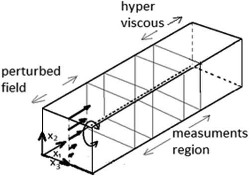
The domain has $4\times 1\times 1$ dimensions. In the first part, $0<x_1\le 1,$ an artificial oscillatory field $f$ induces periodic rotation around line ${(x}_1, x_2)=(0.5,0.5),$ symmetric regarding plane $x_3=0.5:$ (48) $$f=M.\exp \left\{-\left[\frac{{\left(x_1-x_1^O\right)}^2}{{{\sigma }_1}^2}+\frac{{\left(x_2-x_2^O\right)}^2}{{{\sigma }_2}^2}+\frac{{\left(x_3-x_3^O\right)}^2}{{{\sigma }_3}^2}\right]\right\}\left[-\left(x_2-x_2^O\right){\mathit{e}}_1+\left(x_1-x_1^O\right){\mathit{e}}_2\right].\sin \left(2\pi \mu t\right)$$(48) where ${\mathrm{ }x}_i^O=\left(0.5,\mathrm{ }0.5,\mathrm{ }0.5\right),$ $M=2,$ ${\mathrm{ }\sigma }_1={\sigma }_2=0.2,$ ${\sigma }_3=0.4,\mathrm{ }$ and $\mu =0.5.$

Statistics are stored on 18 nodes regularly disposed on two planes, $x_1=1.5$ and $x_1=2.5.$ Attention is focused particularly on node 4, at ${ x}_i=(1.5, 0.5, 0.25).$

In the last part of domain, $3\le x_1<4,$ artificial hyper viscosity reduces the Reynolds number to 10 to enforce a steady flow compatible with homogeneous Newman conditions at outlet.

As already observed, the short domain length is justified in strictly numerical perspective. The measurement planes are close to the perturbed entrance zone and the hyper-viscous outlet zone, where the flow is possibly affected by these artificial zones via pressure. Nevertheless, the measurement interval obeys strictly Navier-Stokes and continuity equations, and possible effects of the artificial zones will not void the numerical testing as such, considering the artificial zones as conditions of this particular problem.

Waiting for the settlement of an almost periodic flow, measurements were taken at each iteration during time range $20\le t\le 30,$ covering five oscillating periods. Negligible differences were noticed in a test in which both waiting time and measurement time were doubled.

Results

Table 1 provides an overall picture of the fluctuating variables for Reynolds number 300, showing eighteen regularly spaced nodes in planes $x_1$= 1.5 and $x_1$= 2.5, as computed with the $240\times 60\times 60$ mesh. Since vorticity is obtained by numerical differentiation, the values of helicity and enstrophy depend on the discretization adopted. Differences between the schemes are small, in few cases reaching the order of 1%. Differences between non-linear and linear UNIFAES discretizations are below 0.01% and cannot be noticed with four significant digits. In almost all cases, the results obtained with UNIFAES are intermediate between the second order central differencing and the forth order central differencing, and is closer to the latter.

Table 1. Characteristic fluctuation parameters in 18 regularly spaced points for Re = 300.

Position		$x_1$ = 1.5			$x_1$ = 2.5
		$x_3$= 0.25	$x_3$ = 0.5	$x_3$= 0.75	$x_3$= 0.25	$x_3$ = 0.5	$x_3$ = 0.75
$x_2$ = .75	Node	7	8	9	16	17	18
	Kin.En.(10^-4)	1.851	2.792	1.851	0.694	0.530	0.694
	Helicity	(10^-3)	(10^-12)	(10^-3)	(10^-3)	(10^-12)	(10^-3)
	CD 2^nd	−1.564	7.309	1.564	−1.098	1.842	1.098
	CD 4^th	−1.561	7.345	1.561	−1.101	1.845	1.101
	Uni NL	−1.562	7.345	1.562	−1.100	1.845	1.100
	Uni L	−1.562	7.345	1.562	−1.100	1.845	1.100
	Enstrophy	(10^-3)	(10^-3)	(10^-3)	(10^-3)	(10^-3)	(10^-3)
	CD 2^nd	7.140	4.620	7.140	8.286	3.157	8.286
	CD 4^th	7.152	4.656	7.152	8.313	3.160	8.313
	Uni NL	7.152	4.651	7.152	8.308	3.161	8.308
	Uni L	7.152	4.651	7.152	8.308	3.161	8.308
$x_2$ =.50	Node	4	5	6	13	14	15
	Kin.En.(10^-4)	5.819	6.298	5.819	0.926	0.587	0.926
	Helicity	(10^-2)	(10^-10)	(10^-2)	(10^-3)	(10^-11)	(10^-3)
	CD 2^nd	−1.221	1.253	1.221	−2.057	5.208	2.057
	CD 4^th	−1.226	1.258	1.226	−2.069	5.232	2.069
	Uni NL	−1.225	1.257	1.225	−2.066	5.227	2.066
	Uni L	−1.225	1.257	1.225	−2.066	5.227	2.066
	Enstrophy	(10^-2)	(10^-2)	(10^-2)	(10^-2)	(10^-2)	(10^-2)
	CD 2^nd	8.633	6.254	8.633	1.256	1.515	1.256
	CD 4^th	8.712	6.305	8.712	1.272	1.524	1.272
	Uni NL	8.695	6.298	8.695	1.268	1.523	1.268
	Uni L	8.695	6.298	8.695	1.268	1.523	1.268
$x_2$ = .25	Node	1	2	3	10	11	12
	Kin.En.(10^-5)	7.303	7.443	7.303	0.289	0.324	0.289
	Helicity	(10^-4)	(10^-11)	(10^-4)	(10^-5)	(10^-12)	(10^-5)
	CD 2^nd	−4.033	1.304	4.033	2.162	−2.607	−2.162
	CD 4^th	−3.984	1.300	3.984	2.199	−2.634	−2.199
	Uni NL	−3.997	1.301	3.997	2.189	−2.628	−2.190
	Uni L	−3.997	1.301	3.997	2.190	−2.628	−2.190
	Enstrophy	(10^-3)	(10^-4)	(10^-3)	(10^-4)	(10^-6)	(10^-4)
	CD 2^nd	3.068	7.259	3.068	1.117	5.649	1.117
	CD 4^th	3.086	7.260	3.086	1.125	5.611	1.125
	Uni NL	3.081	7.261	3.081	1.123	5.620	1.123
	Uni L	3.081	7.261	3.081	1.123	5.620	1.123

Following the symmetry of the initial perturbation, equal values of kinetic energy and enstrophy are observed in planes $x_3$= 0.25 and $x_3$= 0.75, whereas the values of helicity are opposite at those planes and practically nil at central plane $x_3$ = 0.5. Most fluctuating variables decay from measurement planes $x_1$= 1.5 to $x_1$= 2.5, except enstrophy which increases at level $x_2$= 0.75. The sign of helicity inverts between the two measuring planes at level ${ x}_2$= 0.25. Kinetic energy is maximum at symmetry line $x_3$ = 0.5 in measurement plane $x_{1 }$= 1.5, but is minimum at this symmetry line on the upper levels ($x_2$= 0.5 and $x_{2 }$= 0.75) of plane $x_1$= 2.5.

Table 2 shows similar data for Reynolds number 9,600. Differences between schemes are higher, particularly those concerning enstrophy, which reach 34% at node 11; differences in enstrophy between non-linear and linear UNIFAES discretizations reach 13% in node 17. Again, the results of the linear UNIFAES discretizations are usually intermediate between those of CD 2^nd and CD 4^th, and closer to CD 4^th, but the non-linear UNIFAES discretization is often outside this range, and closer to CD 4^th.

Table 2. Characteristic fluctuation parameters in 18 regularly spaced points for Re = 9,600.

Position		$x_1$ = 1.5			$x_1$ = 2.5
		$x_3$= 0.25	$x_3$ = 0.5	$x_3$= 0.75	$x_3$= 0.25	$x_3$ = 0.5	$x_3$ = 0.75
$x_2$ = .75	Node	7	8	9	16	17	18
	Kin.En.(10^-4)	2.788	5.147	2.788	1.922	2.608	1.922
	Helicity	(10^-4)	(10^-9)	(10^-4)	(10^-4)	(10^-9)	(10^-4)
	CD 2^nd	−9.369	3.340	9.369	7.109	−2.053	−7.109
	CD 4^th	−9.195	3.455	9.195	7.773	−3.024	−7.772
	Uni NL	−9.160	3.516	9.160	7.594	−4.258	−7.593
	Uni L	−9.245	3.442	9.245	7.551	−3.206	−7.550
	Enstrophy	(10^-2)	(10^-2)	(10^-2)	(10^-2)	(10^-2)	(10^-2)
	CD 2^nd	2.025	3.353	2.025	3.481	3.466	3.481
	CD 4^th	2.063	3.496	2.063	3.564	4.222	3.564
	Uni NL	2.071	3.583	2.071	3.548	4.929	3.548
	Uni L	2.054	3.476	2.054	3.541	4.274	3.541
$x_2$ =.50	Node	4	5	6	13	14	15
	Kin.En.(10^-4)	2.337	1.999	2.337	1.204	0.425	1.204
	Helicity	(10^-2)	(10^-8)	(10^-2)	(10^-2)	(10^-8)	(10^-2)
	CD 2^nd	−6.068	3.076	6.068	−3.336	2.119	3.336
	CD 4^th	−6.097	3.080	6.097	−3.458	2.172	3.458
	Uni NL	−6.104	3.059	6.104	−3.429	2.190	3.429
	Uni L	−6.094	3.080	6.094	−3.431	2.194	3.431
	Enstrophy	(10^-1)	(10^-1)	(10^-1)	(10^-1)	(10^-1)	(10^-1)
	CD 2^nd	5.226	2.764	5.226	7.804	0.354	7.804
	CD 4^th	5.314	2.822	5.314	8.452	0.418	8.452
	Uni NL	5.342	2.837	5.342	8.391	0.415	8.391
	Uni L	5.303	2.813	5.303	8.314	0.396	8.314
$x_2$ = .25	Node	1	2	3	10	11	12
	Kin.En.(10^-5)	1.722	1.747	1.722	0.546	0.801	0.546
	Helicity	(10^-3)	(10^-9)	(10^-3)	(10^-3)	(10^-9)	(10^-3)
	CD 2^nd	3.271	3.741	−3.271	0.910	−5.007	−0.910
	CD 4^th	4.089	−4.338	−4.089	1.049	−5.961	−1.049
	Uni NL	4.112	−4.250	−4.112	1.024	−6.045	−1.024
	Uni L	4.010	−4.222	−4.010	1.007	−6.144	−1.007
	Enstrophy	(10^-2)	(10^-2)	(10^-2)	(10^-2)	(10^-2)	(10^-2)
	CD 2^nd	4.919	4.098	4.919	0.778	1.130	0.778
	CD 4^th	5.793	4.852	5.793	1.000	1.366	1.000
	Uni NL	5.743	5.333	5.743	0.931	1.681	0.931
	Uni L	5.505	5.105	5.505	0.903	1.713	0.903

Kinetic energy is reduced from all nodes of measurement plane $x_{1 }$= 1.5 to the corresponding nodes at $x_1$= 2.5. But enstrophy increases between these planes at level $x_2$= 0.75. At level $x_2$= 0.5, enstrophy is lower in the symmetry plane $x_3=0.5$ than in planes $x_3=0.25$ and $x_3=0.75,$ and such characteristic is amplified downwind. Helicity changes its sign at the upper level $x_{2 }= 0.75.$

As seen in both low and high Reynolds numbers, the fluctuating scalars of the two measurement planes show structural differences; the stream wise development follows no similarity rule.

Next, the terms of the transport equations are considered for the low Reynolds number case, referring to node 4. Results with the non-linear generalized UNIFAES are not shown, due to its small differences with the linear form in low Reynolds numbers. It is worth reporting that attempts to use nonlinear derivative analogous to Equation(25) $$\widetilde{\frac{\partial u_i}{\partial x_j}}={\tilde{\frac{\partial \left({U_i+u}_i\right)}{\partial x_j}}}_{{U_j+u}_j}\text{-}\mathrm{ }{\widetilde{\frac{\partial U_i}{\partial x_j}}}_{{\mathrm{ }U}_j}$$(25) (25(25) $$\widetilde{\frac{\partial u_i}{\partial x_j}}={\tilde{\frac{\partial \left({U_i+u}_i\right)}{\partial x_j}}}_{{U_j+u}_j}\text{-}\mathrm{ }{\widetilde{\frac{\partial U_i}{\partial x_j}}}_{{\mathrm{ }U}_j}$$(25) )(25) $$\widetilde{\frac{\partial u_i}{\partial x_j}}={\tilde{\frac{\partial \left({U_i+u}_i\right)}{\partial x_j}}}_{{U_j+u}_j}\text{-}\mathrm{ }{\widetilde{\frac{\partial U_i}{\partial x_j}}}_{{\mathrm{ }U}_j}$$(25) for scalars such as kinetic energy or helicity produced unacceptable results, whereas the left sides of Equation(26) $${\mathrm{ }\widetilde{\frac{\partial u_i}{\partial x_j}}}_{{{\mathrm{ }U}_j+u}_j}=\mathrm{ }{\tilde{\frac{\partial \left({U_i+u}_i\right)}{\partial x_j}}}_{{U_j+u}_j}\text{-}\mathrm{ }{\widetilde{\frac{\partial U_i}{\partial x_j}}}_{{{\mathrm{ }U}_j+u}_j}$$(26) (26(26) $${\mathrm{ }\widetilde{\frac{\partial u_i}{\partial x_j}}}_{{{\mathrm{ }U}_j+u}_j}=\mathrm{ }{\tilde{\frac{\partial \left({U_i+u}_i\right)}{\partial x_j}}}_{{U_j+u}_j}\text{-}\mathrm{ }{\widetilde{\frac{\partial U_i}{\partial x_j}}}_{{{\mathrm{ }U}_j+u}_j}$$(26) )(26) $${\mathrm{ }\widetilde{\frac{\partial u_i}{\partial x_j}}}_{{{\mathrm{ }U}_j+u}_j}=\mathrm{ }{\tilde{\frac{\partial \left({U_i+u}_i\right)}{\partial x_j}}}_{{U_j+u}_j}\text{-}\mathrm{ }{\widetilde{\frac{\partial U_i}{\partial x_j}}}_{{{\mathrm{ }U}_j+u}_j}$$(26) and of Equation(27) $${\mathrm{ }\widetilde{\frac{\partial u_i}{\partial x_j}}}_{{\mathrm{ }U}_j}=\mathrm{ }{\tilde{\frac{\partial \left({U_i+u}_i\right)}{\partial x_j}}}_{U_j}\text{-}\mathrm{ }{\widetilde{\frac{\partial U_i}{\partial x_j}}}_{{\mathrm{ }U}_j}$$(27) (27(27) $${\mathrm{ }\widetilde{\frac{\partial u_i}{\partial x_j}}}_{{\mathrm{ }U}_j}=\mathrm{ }{\tilde{\frac{\partial \left({U_i+u}_i\right)}{\partial x_j}}}_{U_j}\text{-}\mathrm{ }{\widetilde{\frac{\partial U_i}{\partial x_j}}}_{{\mathrm{ }U}_j}$$(27) )(27) $${\mathrm{ }\widetilde{\frac{\partial u_i}{\partial x_j}}}_{{\mathrm{ }U}_j}=\mathrm{ }{\tilde{\frac{\partial \left({U_i+u}_i\right)}{\partial x_j}}}_{U_j}\text{-}\mathrm{ }{\widetilde{\frac{\partial U_i}{\partial x_j}}}_{{\mathrm{ }U}_j}$$(27) provided reasonable results. Accordingly, the non-linear derivative analogous to Equation(25) $$\widetilde{\frac{\partial u_i}{\partial x_j}}={\tilde{\frac{\partial \left({U_i+u}_i\right)}{\partial x_j}}}_{{U_j+u}_j}\text{-}\mathrm{ }{\widetilde{\frac{\partial U_i}{\partial x_j}}}_{{\mathrm{ }U}_j}$$(25) (25(25) $$\widetilde{\frac{\partial u_i}{\partial x_j}}={\tilde{\frac{\partial \left({U_i+u}_i\right)}{\partial x_j}}}_{{U_j+u}_j}\text{-}\mathrm{ }{\widetilde{\frac{\partial U_i}{\partial x_j}}}_{{\mathrm{ }U}_j}$$(25) )(25) $$\widetilde{\frac{\partial u_i}{\partial x_j}}={\tilde{\frac{\partial \left({U_i+u}_i\right)}{\partial x_j}}}_{{U_j+u}_j}\text{-}\mathrm{ }{\widetilde{\frac{\partial U_i}{\partial x_j}}}_{{\mathrm{ }U}_j}$$(25) can neither be applied to the Reynolds tensor nor to the velocity-vorticity tensor since it cannot be applied to their traces. Applying the non-linear derivative to vorticity as a vector showed no particular issue; furthermore, although vorticity is also represented by the rotation tensor, it has nil trace, thus the previous argument against using Equation(25) $$\widetilde{\frac{\partial u_i}{\partial x_j}}={\tilde{\frac{\partial \left({U_i+u}_i\right)}{\partial x_j}}}_{{U_j+u}_j}\text{-}\mathrm{ }{\widetilde{\frac{\partial U_i}{\partial x_j}}}_{{\mathrm{ }U}_j}$$(25) (25(25) $$\widetilde{\frac{\partial u_i}{\partial x_j}}={\tilde{\frac{\partial \left({U_i+u}_i\right)}{\partial x_j}}}_{{U_j+u}_j}\text{-}\mathrm{ }{\widetilde{\frac{\partial U_i}{\partial x_j}}}_{{\mathrm{ }U}_j}$$(25) )(25) $$\widetilde{\frac{\partial u_i}{\partial x_j}}={\tilde{\frac{\partial \left({U_i+u}_i\right)}{\partial x_j}}}_{{U_j+u}_j}\text{-}\mathrm{ }{\widetilde{\frac{\partial U_i}{\partial x_j}}}_{{\mathrm{ }U}_j}$$(25) for tensors is not directly applied. One aspect of the nonlinear UNIFAES scheme remains in the following results: the divergence form of the turbulent transport terms (Td) of the scalars with UNIFAES is obtained as the difference between the divergence forms of the mean advective term by using the instantaneous velocity and the mean velocity.

Table 3 shows the various terms of the kinetic energy Equations(43) $$\frac{\partial U_j\overline{u_i{u}_i}/2}{\partial x_j}-\nu \frac{{\partial }^2{\overline{u_{i}u}}_i/2}{\partial x_j\partial x_j}=-\overline{u_i{u}_j}{S}_{ij}\mathrm{ }–\frac{\partial \overline{u_{j}p}}{\partial x_j}-\frac{\partial \overline{u_j{u}_i{u}_i}/2}{\partial x_j}\mathrm{ }-\nu \overline{\frac{\partial u_i}{\partial x_j}\frac{\partial u_i}{\partial x_j}}$$(43) (43(43) $$\frac{\partial U_j\overline{u_i{u}_i}/2}{\partial x_j}-\nu \frac{{\partial }^2{\overline{u_{i}u}}_i/2}{\partial x_j\partial x_j}=-\overline{u_i{u}_j}{S}_{ij}\mathrm{ }–\frac{\partial \overline{u_{j}p}}{\partial x_j}-\frac{\partial \overline{u_j{u}_i{u}_i}/2}{\partial x_j}\mathrm{ }-\nu \overline{\frac{\partial u_i}{\partial x_j}\frac{\partial u_i}{\partial x_j}}$$(43) )(43) $$\frac{\partial U_j\overline{u_i{u}_i}/2}{\partial x_j}-\nu \frac{{\partial }^2{\overline{u_{i}u}}_i/2}{\partial x_j\partial x_j}=-\overline{u_i{u}_j}{S}_{ij}\mathrm{ }–\frac{\partial \overline{u_{j}p}}{\partial x_j}-\frac{\partial \overline{u_j{u}_i{u}_i}/2}{\partial x_j}\mathrm{ }-\nu \overline{\frac{\partial u_i}{\partial x_j}\frac{\partial u_i}{\partial x_j}}$$(43) and (44)(44) $$\frac{\partial U_j\overline{u_i{u}_i/2}}{\partial x_j}-2\nu \frac{\partial \overline{u_i{s}_{ij}}}{\partial x_j}\mathrm{ }=-\overline{u_i{u}_j}{S}_{ij}\mathrm{ }-\frac{\partial \overline{u_{j}p}}{\partial x_j}-\frac{\partial \overline{{u_{j}u}_i{u}_i/2}}{\partial x_j}-2\nu \mathrm{ }\overline{s_{ij}{s}_{ij}}$$(44) . The advective term can be expressed in advective form Aa $=U_j\partial \overline{\left(u_i{u}_i/2\right)}/\partial x_j$ or divergence form Ad $=\partial \left(U_j\overline{u_i{u}_i/2}\right)/\partial x_j,$ which also applies to the turbulent transport and the pressure terms: Ta $=\overline{u_j\partial \left(u_i{u}_i/2\right)/\partial x_j},$ Td $=\partial \overline{\left({u_{j}u}_i{u}_i/2\right)}/\partial x_j,$ Pa $=\mathrm{ }\overline{u_j\partial p/\partial x_j},$ Pd = $\partial \overline{u_{j}p}/\partial x_j$. There is a single production term, P $=\overline{u_i{u}_j}{S}_{ij}.$

Table 3. Statistics of the kinetic energy transport equations for Re = 300 at node 4 with distinct algebraic forms, numerical schemes, and levels of refinement.

Term (or $\ne$)	$160\times 40\times 40$				$240\times 60\times 60$
	CD 2^nd ord.	CD 4^th ord.	Uni L	Spread-ing	CD 2^nd ord.	CD 4^th ord.	Uni L	Spread-ing
Aa (10^-4)	−4.365	−4.364	−4.364	0.0%	−4.328	−4.327	−4.327	0.0%
Ad (10^-4)	−4.366	−4.365	−4.364	0.0%	−4.328	−4.327	−4.327	0.0%
Aa$\ne$Ad	0.0%	0.0%	0.0%		0.0%	0.0%	0.0%
Ta (10^-6)	3.490	3.632	3.613	3.9%	3.482	3.544	3.525	1.7%
Td (10^-6)	3.397	3.592	3.613	6.0%	3.443	3.533	3.525	2.3%
Ta$\ne$Td	2.7%	1.1%	0.0%		1.1%	0.3%	0.0%
Pa (10^-4)	−3.588	−3.596	−3.588	0.2%	−3.470	−3.473	−3.470	0.1%
Pd (10^-4)	−3.467	−3.559	−3.525	2.6%	−3.418	−3.458	−3.443	1.2%
Pa$\ne$Pd	3.4%	1.0%	1.8%		1.5%	0.4%	0.8%
Df (10^-4)	−1.138	−1.148	−1.138	0.9%	−1.107	−1.111	−1.107	0.4%
Du (10^-4)	3.568	3.647	3.633	2.2%	3.486	3.521	3.513	1.0%
Vu (10^-4)	−4.761	−4.796	−4.779	0.7%	−4.617	−4.632	−4.625	0.3%
Vu$\ne$Df-Du	1.2%	0.0%	0.2%		0.5%	0.0%	0.1%
Ws (10^-4)	−3.239	−3.352	−3.325	3.4%	−3.265	−3.316	−3.303	1.5%
Ds (10^-4)	1.251	1.287	1.280	2.8%	1.218	1.233	1.230	1.2%
Vs (10^-4)	−4.639	−4.785	−4.752	3.1%	−4.564	−4.629	−4.613	1.4%
Vs$\ne$Ts-Ds	3.2%	3.1%	3.1%		1.8%	1.7%	1.7%
Vs$\ne$Vu	2.6%	0.2%	0.6%		1.1%	0.1%	0.3%
P (10^-4)	3.381	3.385	3.384	0.1%	3.264	3.266	3.265	0.1%
Resid. Equation(43) $$\frac{\partial U_j\overline{u_i{u}_i}/2}{\partial x_j}-\nu \frac{{\partial }^2{\overline{u_{i}u}}_i/2}{\partial x_j\partial x_j}=-\overline{u_i{u}_j}{S}_{ij}\mathrm{ }–\frac{\partial \overline{u_{j}p}}{\partial x_j}-\frac{\partial \overline{u_j{u}_i{u}_i}/2}{\partial x_j}\mathrm{ }-\nu \overline{\frac{\partial u_i}{\partial x_j}\frac{\partial u_i}{\partial x_j}}$$(43) (43(43) $$\frac{\partial U_j\overline{u_i{u}_i}/2}{\partial x_j}-\nu \frac{{\partial }^2{\overline{u_{i}u}}_i/2}{\partial x_j\partial x_j}=-\overline{u_i{u}_j}{S}_{ij}\mathrm{ }–\frac{\partial \overline{u_{j}p}}{\partial x_j}-\frac{\partial \overline{u_j{u}_i{u}_i}/2}{\partial x_j}\mathrm{ }-\nu \overline{\frac{\partial u_i}{\partial x_j}\frac{\partial u_i}{\partial x_j}}$$(43) )(43) $$\frac{\partial U_j\overline{u_i{u}_i}/2}{\partial x_j}-\nu \frac{{\partial }^2{\overline{u_{i}u}}_i/2}{\partial x_j\partial x_j}=-\overline{u_i{u}_j}{S}_{ij}\mathrm{ }–\frac{\partial \overline{u_{j}p}}{\partial x_j}-\frac{\partial \overline{u_j{u}_i{u}_i}/2}{\partial x_j}\mathrm{ }-\nu \overline{\frac{\partial u_i}{\partial x_j}\frac{\partial u_i}{\partial x_j}}$$(43) (10^-5)	1.680 3.8%	2.558 5.9%	2.375 5.4%		0.945 2.2%	1.326 3.1%	1.235 2.9%
Resid. Equation(44) $$\frac{\partial U_j\overline{u_i{u}_i/2}}{\partial x_j}-2\nu \frac{\partial \overline{u_i{s}_{ij}}}{\partial x_j}\mathrm{ }=-\overline{u_i{u}_j}{S}_{ij}\mathrm{ }-\frac{\partial \overline{u_{j}p}}{\partial x_j}-\frac{\partial \overline{{u_{j}u}_i{u}_i/2}}{\partial x_j}-2\nu \mathrm{ }\overline{s_{ij}{s}_{ij}}$$(44) (44(44) $$\frac{\partial U_j\overline{u_i{u}_i/2}}{\partial x_j}-2\nu \frac{\partial \overline{u_i{s}_{ij}}}{\partial x_j}\mathrm{ }=-\overline{u_i{u}_j}{S}_{ij}\mathrm{ }-\frac{\partial \overline{u_{j}p}}{\partial x_j}-\frac{\partial \overline{{u_{j}u}_i{u}_i/2}}{\partial x_j}-2\nu \mathrm{ }\overline{s_{ij}{s}_{ij}}$$(44) )(44) $$\frac{\partial U_j\overline{u_i{u}_i/2}}{\partial x_j}-2\nu \frac{\partial \overline{u_i{s}_{ij}}}{\partial x_j}\mathrm{ }=-\overline{u_i{u}_j}{S}_{ij}\mathrm{ }-\frac{\partial \overline{u_{j}p}}{\partial x_j}-\frac{\partial \overline{{u_{j}u}_i{u}_i/2}}{\partial x_j}-2\nu \mathrm{ }\overline{s_{ij}{s}_{ij}}$$(44) (10^-5)	-0.478 1.1%	0.991 2.3%	0.722 1.7%		-0.162 0.4%	0.497 1.1%	0.366 0.8%

The two forms of the kinetic energy equation differ regarding the viscous term, each one related to one member of equality Vu = Vs, where Vu $=\upsilon \overline{u_i{\partial }^2{u}_i/\partial x_j\partial x_j}$ and Vs $=2\upsilon \overline{u_i\partial s_{ij}/\partial x_j}$. The viscous term of the first form, Equation(43) $$\frac{\partial U_j\overline{u_i{u}_i}/2}{\partial x_j}-\nu \frac{{\partial }^2{\overline{u_{i}u}}_i/2}{\partial x_j\partial x_j}=-\overline{u_i{u}_j}{S}_{ij}\mathrm{ }–\frac{\partial \overline{u_{j}p}}{\partial x_j}-\frac{\partial \overline{u_j{u}_i{u}_i}/2}{\partial x_j}\mathrm{ }-\nu \overline{\frac{\partial u_i}{\partial x_j}\frac{\partial u_i}{\partial x_j}}$$(43) (43(43) $$\frac{\partial U_j\overline{u_i{u}_i}/2}{\partial x_j}-\nu \frac{{\partial }^2{\overline{u_{i}u}}_i/2}{\partial x_j\partial x_j}=-\overline{u_i{u}_j}{S}_{ij}\mathrm{ }–\frac{\partial \overline{u_{j}p}}{\partial x_j}-\frac{\partial \overline{u_j{u}_i{u}_i}/2}{\partial x_j}\mathrm{ }-\nu \overline{\frac{\partial u_i}{\partial x_j}\frac{\partial u_i}{\partial x_j}}$$(43) )(43) $$\frac{\partial U_j\overline{u_i{u}_i}/2}{\partial x_j}-\nu \frac{{\partial }^2{\overline{u_{i}u}}_i/2}{\partial x_j\partial x_j}=-\overline{u_i{u}_j}{S}_{ij}\mathrm{ }–\frac{\partial \overline{u_{j}p}}{\partial x_j}-\frac{\partial \overline{u_j{u}_i{u}_i}/2}{\partial x_j}\mathrm{ }-\nu \overline{\frac{\partial u_i}{\partial x_j}\frac{\partial u_i}{\partial x_j}}$$(43) , is decomposed according to Vu = Df $-$ Du, where Df $=\upsilon {\partial }^2\overline{{u_{i}u}_i/2 }/\partial x_j\partial x_j$ and Du $=\upsilon \overline{\left(\partial u_i/\partial x_j\right)\left(\partial u_i/\partial x_j\right)}.$ The one of the second form, Equation(44) $$\frac{\partial U_j\overline{u_i{u}_i/2}}{\partial x_j}-2\nu \frac{\partial \overline{u_i{s}_{ij}}}{\partial x_j}\mathrm{ }=-\overline{u_i{u}_j}{S}_{ij}\mathrm{ }-\frac{\partial \overline{u_{j}p}}{\partial x_j}-\frac{\partial \overline{{u_{j}u}_i{u}_i/2}}{\partial x_j}-2\nu \mathrm{ }\overline{s_{ij}{s}_{ij}}$$(44) (44(44) $$\frac{\partial U_j\overline{u_i{u}_i/2}}{\partial x_j}-2\nu \frac{\partial \overline{u_i{s}_{ij}}}{\partial x_j}\mathrm{ }=-\overline{u_i{u}_j}{S}_{ij}\mathrm{ }-\frac{\partial \overline{u_{j}p}}{\partial x_j}-\frac{\partial \overline{{u_{j}u}_i{u}_i/2}}{\partial x_j}-2\nu \mathrm{ }\overline{s_{ij}{s}_{ij}}$$(44) )(44) $$\frac{\partial U_j\overline{u_i{u}_i/2}}{\partial x_j}-2\nu \frac{\partial \overline{u_i{s}_{ij}}}{\partial x_j}\mathrm{ }=-\overline{u_i{u}_j}{S}_{ij}\mathrm{ }-\frac{\partial \overline{u_{j}p}}{\partial x_j}-\frac{\partial \overline{{u_{j}u}_i{u}_i/2}}{\partial x_j}-2\nu \mathrm{ }\overline{s_{ij}{s}_{ij}}$$(44) , is decomposed according to Vs = Ws $-$ Ds, where Ws $=\upsilon \partial \overline{u_i{s}_{ij}}/\partial x_j$ and Ds $=\upsilon \overline{s_{ij}{s}_{ij}}.$

Differences between algebraic forms and the spreading of results according to the schemes are expressed, in italic, as percentage of the term with higher module in each relation.

The $160\times 40\times 40$ and $240\times 60\times 60$ meshes show close results, with differences generally within 3%. All schemes show remarkable proximity in both advective and divergence forms of the mean advective term. Most often, the differences between distinct algebraic forms and the spreading of results according to the schemes reduce from the $160\times 40\times 40$ to the $240\times 60\times 60$ meshes in a proportion close to 9:4, as expected for quadratic behavior. Differences between distinct algebraic forms of CD 4^th are often expressively smaller than corresponding differences for other schemes, reflecting its superior order. Again, results with linear generalized UNIFAES are usually closer to CD 4^th than to CD 2^nd.

The two last lines show the residuals of the Equations(43) $$\frac{\partial U_j\overline{u_i{u}_i}/2}{\partial x_j}-\nu \frac{{\partial }^2{\overline{u_{i}u}}_i/2}{\partial x_j\partial x_j}=-\overline{u_i{u}_j}{S}_{ij}\mathrm{ }–\frac{\partial \overline{u_{j}p}}{\partial x_j}-\frac{\partial \overline{u_j{u}_i{u}_i}/2}{\partial x_j}\mathrm{ }-\nu \overline{\frac{\partial u_i}{\partial x_j}\frac{\partial u_i}{\partial x_j}}$$(43) (43(43) $$\frac{\partial U_j\overline{u_i{u}_i}/2}{\partial x_j}-\nu \frac{{\partial }^2{\overline{u_{i}u}}_i/2}{\partial x_j\partial x_j}=-\overline{u_i{u}_j}{S}_{ij}\mathrm{ }–\frac{\partial \overline{u_{j}p}}{\partial x_j}-\frac{\partial \overline{u_j{u}_i{u}_i}/2}{\partial x_j}\mathrm{ }-\nu \overline{\frac{\partial u_i}{\partial x_j}\frac{\partial u_i}{\partial x_j}}$$(43) )(43) $$\frac{\partial U_j\overline{u_i{u}_i}/2}{\partial x_j}-\nu \frac{{\partial }^2{\overline{u_{i}u}}_i/2}{\partial x_j\partial x_j}=-\overline{u_i{u}_j}{S}_{ij}\mathrm{ }–\frac{\partial \overline{u_{j}p}}{\partial x_j}-\frac{\partial \overline{u_j{u}_i{u}_i}/2}{\partial x_j}\mathrm{ }-\nu \overline{\frac{\partial u_i}{\partial x_j}\frac{\partial u_i}{\partial x_j}}$$(43) and (44)(44) $$\frac{\partial U_j\overline{u_i{u}_i/2}}{\partial x_j}-2\nu \frac{\partial \overline{u_i{s}_{ij}}}{\partial x_j}\mathrm{ }=-\overline{u_i{u}_j}{S}_{ij}\mathrm{ }-\frac{\partial \overline{u_{j}p}}{\partial x_j}-\frac{\partial \overline{{u_{j}u}_i{u}_i/2}}{\partial x_j}-2\nu \mathrm{ }\overline{s_{ij}{s}_{ij}}$$(44) using the divergence forms of mean and turbulent advective terms, for coherence with the Navier-Stokes solver, and the advective form of the pressure equation, which directly emerges in deriving the equation. The residuals are also expressed as percentage of the greatest term of the equation in modulus, which is mean advection. Paradoxically, the smallest residuals are those of CD 2^nd, which showed the highest differences between distinct algebraic forms, and the greatest residuals are those of CD 4^th, with the smallest differences between algebraic forms. The residuals of Equation(44) $$\frac{\partial U_j\overline{u_i{u}_i/2}}{\partial x_j}-2\nu \frac{\partial \overline{u_i{s}_{ij}}}{\partial x_j}\mathrm{ }=-\overline{u_i{u}_j}{S}_{ij}\mathrm{ }-\frac{\partial \overline{u_{j}p}}{\partial x_j}-\frac{\partial \overline{{u_{j}u}_i{u}_i/2}}{\partial x_j}-2\nu \mathrm{ }\overline{s_{ij}{s}_{ij}}$$(44) (44(44) $$\frac{\partial U_j\overline{u_i{u}_i/2}}{\partial x_j}-2\nu \frac{\partial \overline{u_i{s}_{ij}}}{\partial x_j}\mathrm{ }=-\overline{u_i{u}_j}{S}_{ij}\mathrm{ }-\frac{\partial \overline{u_{j}p}}{\partial x_j}-\frac{\partial \overline{{u_{j}u}_i{u}_i/2}}{\partial x_j}-2\nu \mathrm{ }\overline{s_{ij}{s}_{ij}}$$(44) )(44) $$\frac{\partial U_j\overline{u_i{u}_i/2}}{\partial x_j}-2\nu \frac{\partial \overline{u_i{s}_{ij}}}{\partial x_j}\mathrm{ }=-\overline{u_i{u}_j}{S}_{ij}\mathrm{ }-\frac{\partial \overline{u_{j}p}}{\partial x_j}-\frac{\partial \overline{{u_{j}u}_i{u}_i/2}}{\partial x_j}-2\nu \mathrm{ }\overline{s_{ij}{s}_{ij}}$$(44) behave roughly in second order, but those of Equation(43) $$\frac{\partial U_j\overline{u_i{u}_i}/2}{\partial x_j}-\nu \frac{{\partial }^2{\overline{u_{i}u}}_i/2}{\partial x_j\partial x_j}=-\overline{u_i{u}_j}{S}_{ij}\mathrm{ }–\frac{\partial \overline{u_{j}p}}{\partial x_j}-\frac{\partial \overline{u_j{u}_i{u}_i}/2}{\partial x_j}\mathrm{ }-\nu \overline{\frac{\partial u_i}{\partial x_j}\frac{\partial u_i}{\partial x_j}}$$(43) (43(43) $$\frac{\partial U_j\overline{u_i{u}_i}/2}{\partial x_j}-\nu \frac{{\partial }^2{\overline{u_{i}u}}_i/2}{\partial x_j\partial x_j}=-\overline{u_i{u}_j}{S}_{ij}\mathrm{ }–\frac{\partial \overline{u_{j}p}}{\partial x_j}-\frac{\partial \overline{u_j{u}_i{u}_i}/2}{\partial x_j}\mathrm{ }-\nu \overline{\frac{\partial u_i}{\partial x_j}\frac{\partial u_i}{\partial x_j}}$$(43) )(43) $$\frac{\partial U_j\overline{u_i{u}_i}/2}{\partial x_j}-\nu \frac{{\partial }^2{\overline{u_{i}u}}_i/2}{\partial x_j\partial x_j}=-\overline{u_i{u}_j}{S}_{ij}\mathrm{ }–\frac{\partial \overline{u_{j}p}}{\partial x_j}-\frac{\partial \overline{u_j{u}_i{u}_i}/2}{\partial x_j}\mathrm{ }-\nu \overline{\frac{\partial u_i}{\partial x_j}\frac{\partial u_i}{\partial x_j}}$$(43) do not.

Table 4 shows the terms of the helicity equation. Advection terms admit advective and divergence forms: Aa = $U_j\partial \overline{u_i{w}_i}/\partial x_j,$ Ad = $\partial \left(U_j\overline{u_i{w}_i}\right)/\partial x_j,$ Ta $=\overline{u_j\partial \left(u_i{w}_i\right)/\partial x_j}$ and Td =$\partial \overline{u_i{w}_i{u}_j}/\partial x_j.$ This also holds for the pressure term, since vorticity is also solenoidal: Pa =$\overline{w_j\partial p/\partial x_j}$ and Pd =$\overline{\partial \left(p{w}_j\right)/\partial x_j}.$ Two production terms by interaction between mean and fluctuating velocity fields exist: P1 =${\partial \left(u_i{u}_j\right)/\partial x_{j}W}_i$ and P2 $=\overline{u_i{u}_j}\partial W_i/\partial x_j.$ The strictly fluctuating production term admits distinct algebraic forms, including Pt1 $=\overline{u_i{w}_j{s}_{ij}},$ Pt2 = $\overline{w_j\partial \left(u_i{u}_i/2\right)/\partial x_j},$ and Pt3 = $\partial \left(\overline{{w_{j}u}_i{u}_i}/2\right)/\partial x_j.$ For the viscous terms, the helicity transport equation required the equality V = Df $-$ Ds, where V $=\upsilon \left(\overline{u_i{\partial }^2{w}_i/\partial x_j\partial x_j}+\overline{w_i{\partial }^2{u}_i/\partial x_j\partial x_j}\right),$ Df $=\upsilon {\partial }^2\overline{{u_{i}w}_i}/\partial x_j\partial x_j,$ and Ds $=\upsilon \overline{\left(\partial u_i/\partial x_j\right)\left(\partial w_i/\partial x_j\right)}.$

Table 4. Statistics of the transport equation for helicity for Re = 300 at node 4 with distinct algebraic forms, numerical schemes, and levels of refinement.

Term (or $\ne$)	$160\times 40\times 40$				$240\times 60\times 60$
	CD 2^ndord.	CD 4^th ord.	Uni L	Spread-ing	CD 2^nd ord.	CD 4^th ord.	Uni L	Spread-ing
Aa (10^-3)	7.510	7.548	7.549	0.5%	7.473	7.490	7.489	0.2%
Ad (10^-3)	7.511	7.549	7.549	0.5%	7.474	7.491	7.489	0.2%
Aa$\ne$Ad	0.0%	0.0%	0.0%		0.0%	0.0%	0.0%
Ta (10^-5)	−4.203	−4.759	−4.633	11.7%	−4.642	−4.904	−4.842	5.3%
Td (10^-5)	−4.326	−4.797	−4.744	9.8%	−4.696	−4.921	−4.861	4.6%
Ta$\ne$Td	2.8%	0.8%	2.3%		1.1%	0.3%	0.4%
Pa (10^-3)	7.160	7.273	7.229	1.6%	7.038	7.088	7.069	0.7%
Pd (10^-3)	7.132	7.272	7.227	1.9%	7.026	7.088	7.065	0.9%
Pa$\ne$Pd	0.5%	0.0%	0.0%		0.2%	0.0%	0.1%
Df (10^-3)	4.761	4.841	4.804	1.7%	4.633	4.668	4.648	0.7%
Du (10^-3)	−7.941	−8.175	−8.110	2.9%	−7.759	−7.861	−7.829	1.3%
V (10^-3)	12.757	13.022	12.914	2.0%	12.415	12.529	12.482	0.9%
V$\ne$Df-Du	0.4%	0.0%	0.0%		0.2%	0.0%	0.0%
P1 (10^-3)	2.004	2.046	2.035	2.1%	1.968	1.986	1.981	0.9%
P2 (10^-4)	−3.614	−3.718	−3.692	2.8%	−3.552	−3.598	−3.586	1.3%
Pt1 (10^-6)	−7.175	−8.862	−8.111	19.0%	−9.016	−9.798	−9.522	8.0%
Pt2 (10^-6)	−7.011	−8.918	−8.651	21.4%	−8.956	−9.810	−9.647	8.7%
Pt3 (10^-6)	−7.387	−8.887	−8.828	16.9%	−9.115	−9.803	−9.726	7.0%
$\ne$Pt123	5.1%	0.6%	8.1%		1.7%	0.1%	2.1%
Resid. Eq.(45)(45) $$\frac{\partial \overline{u_i{w}_i}{U}_j}{\partial x_j}-\nu \frac{{\partial }^2\overline{{u_{i}w}_i}}{\partial x_j\partial x_j}={\overline{\frac{\partial u_i{u}_j}{\partial x_j}}W}_i-\overline{u_i{u}_j}\frac{\partial W_i}{\partial x_j}-\overline{w_i\frac{\partial p}{\partial x_i}}+\overline{u_i{w}_j{s}_{ij}}-\frac{\partial \overline{u_i{w}_i{u}_j}}{\partial x_j}-2\nu \overline{\frac{\partial u_i}{\partial x_j}\frac{\partial w_i}{\partial x_j}}$$(45) (10^-4)	-4.324 5.4%	-6.515 8.0%	-5.779 7.1%		-2.406 3.1%	-3.350 4.3%	-2.987 3.8%

Table 5 refers to enstrophy equation. Mean and turbulent advection terms have advective and divergence forms: Aa =$\mathrm{ }\partial \left(U_j\overline{w_i{w}_i/2}\right)/\partial x_j,$ Ad =$\mathrm{ }{U}_j\partial \overline{w_i{w}_i/2}/\partial x_j,$ Ta =$\overline{{\mathrm{ }u}_j\partial \left(w_i{w}_i/2\right)/\partial x_j}$ and Td =$\mathrm{ }\partial \overline{u_j{w}_i{w}_i/2}/\partial x_j.$ The viscous terms of the enstrophy equation result from identity V = Df $\text{-}$ Ds, where V $=\mathrm{ }\upsilon \overline{w_i{\partial }^2{w}_i/\partial x_j\partial x_j},$ Df $=\upsilon {\partial }^2\left(\overline{{w_{i}w}_i}/2\right)/\partial x_j\partial x_j$ and Ds $=\upsilon \overline{\left(\partial w_i/\partial x_j\right)\left(\partial w_i/\partial x_j\right)}.$ There are three terms of production by interaction between mean and fluctuating field, P1 $=\overline{w_i{u}_j}\partial W_i/\partial x_j,$ P2 $=\overline{w_i{w}_j}{S}_{ij}$ and P3 $=\overline{w_i{s}_{ij}}{W}_j,$ and one production term due to the fluctuation field only, Pt = $\overline{w_i{w}_j{s}_{ij}}.$

Table 5. Statistics of the transport equation for enstrophy for Re = 300 at node 4 with distinct algebraic forms, numerical schemes, and levels of refinement.

Term (or $\ne )$	$160\times 40\times 40$				$240\times 60\times 60$
	CD 2^nd ord.	CD 4^th ord.	Uni L	Spread-ing	CD 2^nd ord.	CD 4^th ord.	Uni L	Spread-ing
Aa (10^-2)	−7.181	−7.296	−7.280	1.6%	−7.141	−7.191	−7.181	0.7%
Ad (10^-2)	−7.182	−7.297	−7.280	1.6%	−7.141	−7.191	−7.181	0.7%
Aa$\ne$Ad	0.0%	0.0%	0.0%		0.0%	0.0%	0.0%
Ta (10^-4)	3.745	5.062	4.703	26.0%	4.629	5.245	5.085	11.7%
Td (10^-4)	4.178	5.199	4.866	19.6%	4.814	5.291	5.125	9.0%
Ta$\ne$Td	10.4%	2.6%	3.3%		3.8%	0.9%	0.8%
Df (10^-2)	−3.598	−3.741	−3.676	3.8%	−3.523	−3.584	−3.553	1.7%
Du (10^-2)	6.024	6.418	6.334	6.1%	5.962	6.134	6.095	2.8%
V (10^-2)	−9.769	−10.166	−10.030	3.9%	−9.549	−9.720	−9.660	1.8%
V$\ne$Df-Du	1.5%	0.1%	0.2%		0.7%	0.0%	0.1%
P1 (10^-3)	4.020	4.214	4.165	4.6%	3.969	4.054	4.032	2.1%
P2 (10^-2)	3.140	3.195	3.185	1.7%	3.072	3.096	3.091	0.8%
P3 (10^-3)	−3.667	−3.826	−3.775	4.2%	−3.600	−3.670	−3.650	1.9%
Pt (10^-4)	−1.757	−1.707	−1.761	3.1%	−1.490	−1.463	−1.480	1.8%
Resid. Equation(46) $$\frac{\partial U_j\overline{w_i{w}_i/2}}{\partial x_j}-\upsilon \frac{{\partial }^2\overline{{w_{i}w}_i}/2}{\partial x_j\partial x_j}=\overline{w_i{s}_{ij}}{W}_j+\overline{w_i{w}_j}{S}_{ij}-\overline{w_i{u}_j}\frac{\partial W_i}{\partial x_j}-\frac{\partial \overline{u_j{w}_i{w}_i/2}}{\partial x_j}\text{-}\mathrm{ }\overline{w_i{w}_j{s}_{ij}}\mathrm{ }-\upsilon \overline{\frac{\partial w_i}{\partial x_j}\frac{\partial w_i}{\partial x_j}}$$(46) (46(46) $$\frac{\partial U_j\overline{w_i{w}_i/2}}{\partial x_j}-\upsilon \frac{{\partial }^2\overline{{w_{i}w}_i}/2}{\partial x_j\partial x_j}=\overline{w_i{s}_{ij}}{W}_j+\overline{w_i{w}_j}{S}_{ij}-\overline{w_i{u}_j}\frac{\partial W_i}{\partial x_j}-\frac{\partial \overline{u_j{w}_i{w}_i/2}}{\partial x_j}\text{-}\mathrm{ }\overline{w_i{w}_j{s}_{ij}}\mathrm{ }-\upsilon \overline{\frac{\partial w_i}{\partial x_j}\frac{\partial w_i}{\partial x_j}}$$(46) )(46) $$\frac{\partial U_j\overline{w_i{w}_i/2}}{\partial x_j}-\upsilon \frac{{\partial }^2\overline{{w_{i}w}_i}/2}{\partial x_j\partial x_j}=\overline{w_i{s}_{ij}}{W}_j+\overline{w_i{w}_j}{S}_{ij}-\overline{w_i{u}_j}\frac{\partial W_i}{\partial x_j}-\frac{\partial \overline{u_j{w}_i{w}_i/2}}{\partial x_j}\text{-}\mathrm{ }\overline{w_i{w}_j{s}_{ij}}\mathrm{ }-\upsilon \overline{\frac{\partial w_i}{\partial x_j}\frac{\partial w_i}{\partial x_j}}$$(46) (10^-3)	0.887 1.2%	5.049 6.9%	3.688 5.1%		0.605 0.8%	2.414 3.4%	1.802 2.5%

For both helicity and enstrophy equations, as well as for the kinetic energy equations, the differences between algebraic forms and between the schemes reduce from the $160\times 40\times 40$ mesh to the $240\times 60\times 60$ mesh in ratios generally close to 9:4, as expected for quadratic behavior. Also, differences between distinct algebraic forms of these terms by using CD 4^th are the smallest among the schemes, respective differences with CD 2^nd are the greatest, and with UNIFAES are intermediate.

The reference term for the helicity equation residuals is dissipation and for the enstrophy equation is advection. Again, these residuals appear not to reduce in quadratic fashion and, again, the smaller residuals correspond to CD 2^nd, which presented the greatest differences between algebraic forms. This apparent contradiction observed in node 4 is not general: CD 2^nd produced the smallest residuals in most nodes, but not all: in node 2, UNIFAES showed the smallest residuals; in many other nodes the scheme with the smallest residuals depended on the equation considered. Anyway, the quickest convergence of CD 2^nd in most nodes must not be attributed the scheme alone, because convergence also depends on the Navier Stokes solver. An extreme example is the advective term of the kinetic energy equations on node 4, to which all schemes practically coincided in the finite meshes, so that all variations of this term with refinement are attributable to the solver.

Interpreting the UNIFAES generalized discretizations, constructed upon the same interpolating curve of the Navier-Stokes solver, as reference for the solver convergence errors, the departure of CD 2^nd from the solver compensated in great part the solver convergence error, whereas the small departure of CD 4^th added to the solver error, for node 4 and many others. For node 2, in which UNIFAES presented the smallest residuals, the errors of both Central Differencing schemes added to the solver error.

Table 6 provides a detailed analysis of the residuals of node 4, registering their values at three refinement levels, $160\times 40\times 40,\mathrm{ }192\times 48\times 48,$ and $240\times 60\times 60,$ and three types of Richardson extrapolations: the first type assumes second order dominance and uses $160\times 40\times 40$ and $240\times 60\times 60$ meshes, the others employ the three meshes to fit two dominating terms, either first and second orders or second and third orders. The left column registers the unit of the data and a reference expressing the order of magnitude of the greatest term of the equation in modulus at the most refined mesh.

Table 6. Residuals of transport equations at finite meshes and extrapolations, Re = 300, node 4.

Transport Equations	Schemes	Meshes			Extrapolations
		160 $\times$ 40$\mathrm{ }\times$ 40	192$\mathrm{ }\times$ 48 $\times$ 48	240$\mathrm{ }\times$ 60$\mathrm{ }\times$ 60	2nd	1st & 2nd	2nd & 3rd
Kin. Energy Equation(43) $$\frac{\partial U_j\overline{u_i{u}_i}/2}{\partial x_j}-\nu \frac{{\partial }^2{\overline{u_{i}u}}_i/2}{\partial x_j\partial x_j}=-\overline{u_i{u}_j}{S}_{ij}\mathrm{ }–\frac{\partial \overline{u_{j}p}}{\partial x_j}-\frac{\partial \overline{u_j{u}_i{u}_i}/2}{\partial x_j}\mathrm{ }-\nu \overline{\frac{\partial u_i}{\partial x_j}\frac{\partial u_i}{\partial x_j}}$$(43) (43(43) $$\frac{\partial U_j\overline{u_i{u}_i}/2}{\partial x_j}-\nu \frac{{\partial }^2{\overline{u_{i}u}}_i/2}{\partial x_j\partial x_j}=-\overline{u_i{u}_j}{S}_{ij}\mathrm{ }–\frac{\partial \overline{u_{j}p}}{\partial x_j}-\frac{\partial \overline{u_j{u}_i{u}_i}/2}{\partial x_j}\mathrm{ }-\nu \overline{\frac{\partial u_i}{\partial x_j}\frac{\partial u_i}{\partial x_j}}$$(43) )(43) $$\frac{\partial U_j\overline{u_i{u}_i}/2}{\partial x_j}-\nu \frac{{\partial }^2{\overline{u_{i}u}}_i/2}{\partial x_j\partial x_j}=-\overline{u_i{u}_j}{S}_{ij}\mathrm{ }–\frac{\partial \overline{u_{j}p}}{\partial x_j}-\frac{\partial \overline{u_j{u}_i{u}_i}/2}{\partial x_j}\mathrm{ }-\nu \overline{\frac{\partial u_i}{\partial x_j}\frac{\partial u_i}{\partial x_j}}$$(43) Unit : 10^-5, Ref. : 4.4 × 10^-4	CD 2^nd	1.680	1.425	0.945	0.357	−0.777	0.195
	CD 4^th	2.558	2.023	1.326	0.341	−1.320	0.185
	Unif. L	2.375	1.890	1.235	0.323	−1.234	0.169
Kin. Energy Eq.(44)(44) $$\frac{\partial U_j\overline{u_i{u}_i/2}}{\partial x_j}-2\nu \frac{\partial \overline{u_i{s}_{ij}}}{\partial x_j}\mathrm{ }=-\overline{u_i{u}_j}{S}_{ij}\mathrm{ }-\frac{\partial \overline{u_{j}p}}{\partial x_j}-\frac{\partial \overline{{u_{j}u}_i{u}_i/2}}{\partial x_j}-2\nu \mathrm{ }\overline{s_{ij}{s}_{ij}}$$(44) Unit : 10^-5, Ref. : 4.4 × 10^-4	CD 2^nd	−0.478	−0.158	−0.162	0.091	0.106	−0.068
	CD 4^th	0.991	0.861	0.497	0.101	−0.754	−0.053
	Unif. L	0.722	0.667	0.366	0.082	−0.620	−0.071
Helicity Equation(45) $$\frac{\partial \overline{u_i{w}_i}{U}_j}{\partial x_j}-\nu \frac{{\partial }^2\overline{{u_{i}w}_i}}{\partial x_j\partial x_j}={\overline{\frac{\partial u_i{u}_j}{\partial x_j}}W}_i-\overline{u_i{u}_j}\frac{\partial W_i}{\partial x_j}-\overline{w_i\frac{\partial p}{\partial x_i}}+\overline{u_i{w}_j{s}_{ij}}-\frac{\partial \overline{u_i{w}_i{u}_j}}{\partial x_j}-2\nu \overline{\frac{\partial u_i}{\partial x_j}\frac{\partial w_i}{\partial x_j}}$$(45) (45(45) $$\frac{\partial \overline{u_i{w}_i}{U}_j}{\partial x_j}-\nu \frac{{\partial }^2\overline{{u_{i}w}_i}}{\partial x_j\partial x_j}={\overline{\frac{\partial u_i{u}_j}{\partial x_j}}W}_i-\overline{u_i{u}_j}\frac{\partial W_i}{\partial x_j}-\overline{w_i\frac{\partial p}{\partial x_i}}+\overline{u_i{w}_j{s}_{ij}}-\frac{\partial \overline{u_i{w}_i{u}_j}}{\partial x_j}-2\nu \overline{\frac{\partial u_i}{\partial x_j}\frac{\partial w_i}{\partial x_j}}$$(45) )(45) $$\frac{\partial \overline{u_i{w}_i}{U}_j}{\partial x_j}-\nu \frac{{\partial }^2\overline{{u_{i}w}_i}}{\partial x_j\partial x_j}={\overline{\frac{\partial u_i{u}_j}{\partial x_j}}W}_i-\overline{u_i{u}_j}\frac{\partial W_i}{\partial x_j}-\overline{w_i\frac{\partial p}{\partial x_i}}+\overline{u_i{w}_j{s}_{ij}}-\frac{\partial \overline{u_i{w}_i{u}_j}}{\partial x_j}-2\nu \overline{\frac{\partial u_i}{\partial x_j}\frac{\partial w_i}{\partial x_j}}$$(45) Unit : 10^-4, Ref. : 7.5 × 10^-3	CD 2^nd	−4.324	−3.624	−2.406	−0.872	2.009	−0.487
	CD 4^th	−6.515	−5.115	−3.350	−0.818	3.388	−0.448
	Unif. L	−5.779	−4.606	−2.987	−0.753	3.098	−0.359
Enstrophy Equation(46) $$\frac{\partial U_j\overline{w_i{w}_i/2}}{\partial x_j}-\upsilon \frac{{\partial }^2\overline{{w_{i}w}_i}/2}{\partial x_j\partial x_j}=\overline{w_i{s}_{ij}}{W}_j+\overline{w_i{w}_j}{S}_{ij}-\overline{w_i{u}_j}\frac{\partial W_i}{\partial x_j}-\frac{\partial \overline{u_j{w}_i{w}_i/2}}{\partial x_j}\text{-}\mathrm{ }\overline{w_i{w}_j{s}_{ij}}\mathrm{ }-\upsilon \overline{\frac{\partial w_i}{\partial x_j}\frac{\partial w_i}{\partial x_j}}$$(46) (46(46) $$\frac{\partial U_j\overline{w_i{w}_i/2}}{\partial x_j}-\upsilon \frac{{\partial }^2\overline{{w_{i}w}_i}/2}{\partial x_j\partial x_j}=\overline{w_i{s}_{ij}}{W}_j+\overline{w_i{w}_j}{S}_{ij}-\overline{w_i{u}_j}\frac{\partial W_i}{\partial x_j}-\frac{\partial \overline{u_j{w}_i{w}_i/2}}{\partial x_j}\text{-}\mathrm{ }\overline{w_i{w}_j{s}_{ij}}\mathrm{ }-\upsilon \overline{\frac{\partial w_i}{\partial x_j}\frac{\partial w_i}{\partial x_j}}$$(46) )(46) $$\frac{\partial U_j\overline{w_i{w}_i/2}}{\partial x_j}-\upsilon \frac{{\partial }^2\overline{{w_{i}w}_i}/2}{\partial x_j\partial x_j}=\overline{w_i{s}_{ij}}{W}_j+\overline{w_i{w}_j}{S}_{ij}-\overline{w_i{u}_j}\frac{\partial W_i}{\partial x_j}-\frac{\partial \overline{u_j{w}_i{w}_i/2}}{\partial x_j}\text{-}\mathrm{ }\overline{w_i{w}_j{s}_{ij}}\mathrm{ }-\upsilon \overline{\frac{\partial w_i}{\partial x_j}\frac{\partial w_i}{\partial x_j}}$$(46) Unit : 10^-3, Ref. : 7.2 × 10^-2	CD 2^nd	0.887	0.999	0.605	0.380	−0.525	0.090
	CD 4^th	5.049	3.845	2.414	0.307	−3.109	0.040
	Unif. L	3.688	2.920	1.802	0.294	−2.361	0.001

Considering the various schemes, the maximum unbalances at the most refined mesh correspond to 3.5% of the reference for Equation(43) $$\frac{\partial U_j\overline{u_i{u}_i}/2}{\partial x_j}-\nu \frac{{\partial }^2{\overline{u_{i}u}}_i/2}{\partial x_j\partial x_j}=-\overline{u_i{u}_j}{S}_{ij}\mathrm{ }–\frac{\partial \overline{u_{j}p}}{\partial x_j}-\frac{\partial \overline{u_j{u}_i{u}_i}/2}{\partial x_j}\mathrm{ }-\nu \overline{\frac{\partial u_i}{\partial x_j}\frac{\partial u_i}{\partial x_j}}$$(43) (43(43) $$\frac{\partial U_j\overline{u_i{u}_i}/2}{\partial x_j}-\nu \frac{{\partial }^2{\overline{u_{i}u}}_i/2}{\partial x_j\partial x_j}=-\overline{u_i{u}_j}{S}_{ij}\mathrm{ }–\frac{\partial \overline{u_{j}p}}{\partial x_j}-\frac{\partial \overline{u_j{u}_i{u}_i}/2}{\partial x_j}\mathrm{ }-\nu \overline{\frac{\partial u_i}{\partial x_j}\frac{\partial u_i}{\partial x_j}}$$(43) )(43) $$\frac{\partial U_j\overline{u_i{u}_i}/2}{\partial x_j}-\nu \frac{{\partial }^2{\overline{u_{i}u}}_i/2}{\partial x_j\partial x_j}=-\overline{u_i{u}_j}{S}_{ij}\mathrm{ }–\frac{\partial \overline{u_{j}p}}{\partial x_j}-\frac{\partial \overline{u_j{u}_i{u}_i}/2}{\partial x_j}\mathrm{ }-\nu \overline{\frac{\partial u_i}{\partial x_j}\frac{\partial u_i}{\partial x_j}}$$(43) , 1.1% for Equation(44) $$\frac{\partial U_j\overline{u_i{u}_i/2}}{\partial x_j}-2\nu \frac{\partial \overline{u_i{s}_{ij}}}{\partial x_j}\mathrm{ }=-\overline{u_i{u}_j}{S}_{ij}\mathrm{ }-\frac{\partial \overline{u_{j}p}}{\partial x_j}-\frac{\partial \overline{{u_{j}u}_i{u}_i/2}}{\partial x_j}-2\nu \mathrm{ }\overline{s_{ij}{s}_{ij}}$$(44) (44(44) $$\frac{\partial U_j\overline{u_i{u}_i/2}}{\partial x_j}-2\nu \frac{\partial \overline{u_i{s}_{ij}}}{\partial x_j}\mathrm{ }=-\overline{u_i{u}_j}{S}_{ij}\mathrm{ }-\frac{\partial \overline{u_{j}p}}{\partial x_j}-\frac{\partial \overline{{u_{j}u}_i{u}_i/2}}{\partial x_j}-2\nu \mathrm{ }\overline{s_{ij}{s}_{ij}}$$(44) )(44) $$\frac{\partial U_j\overline{u_i{u}_i/2}}{\partial x_j}-2\nu \frac{\partial \overline{u_i{s}_{ij}}}{\partial x_j}\mathrm{ }=-\overline{u_i{u}_j}{S}_{ij}\mathrm{ }-\frac{\partial \overline{u_{j}p}}{\partial x_j}-\frac{\partial \overline{{u_{j}u}_i{u}_i/2}}{\partial x_j}-2\nu \mathrm{ }\overline{s_{ij}{s}_{ij}}$$(44) , 4.5% for Equation(45) $$\frac{\partial \overline{u_i{w}_i}{U}_j}{\partial x_j}-\nu \frac{{\partial }^2\overline{{u_{i}w}_i}}{\partial x_j\partial x_j}={\overline{\frac{\partial u_i{u}_j}{\partial x_j}}W}_i-\overline{u_i{u}_j}\frac{\partial W_i}{\partial x_j}-\overline{w_i\frac{\partial p}{\partial x_i}}+\overline{u_i{w}_j{s}_{ij}}-\frac{\partial \overline{u_i{w}_i{u}_j}}{\partial x_j}-2\nu \overline{\frac{\partial u_i}{\partial x_j}\frac{\partial w_i}{\partial x_j}}$$(45) (45(45) $$\frac{\partial \overline{u_i{w}_i}{U}_j}{\partial x_j}-\nu \frac{{\partial }^2\overline{{u_{i}w}_i}}{\partial x_j\partial x_j}={\overline{\frac{\partial u_i{u}_j}{\partial x_j}}W}_i-\overline{u_i{u}_j}\frac{\partial W_i}{\partial x_j}-\overline{w_i\frac{\partial p}{\partial x_i}}+\overline{u_i{w}_j{s}_{ij}}-\frac{\partial \overline{u_i{w}_i{u}_j}}{\partial x_j}-2\nu \overline{\frac{\partial u_i}{\partial x_j}\frac{\partial w_i}{\partial x_j}}$$(45) )(45) $$\frac{\partial \overline{u_i{w}_i}{U}_j}{\partial x_j}-\nu \frac{{\partial }^2\overline{{u_{i}w}_i}}{\partial x_j\partial x_j}={\overline{\frac{\partial u_i{u}_j}{\partial x_j}}W}_i-\overline{u_i{u}_j}\frac{\partial W_i}{\partial x_j}-\overline{w_i\frac{\partial p}{\partial x_i}}+\overline{u_i{w}_j{s}_{ij}}-\frac{\partial \overline{u_i{w}_i{u}_j}}{\partial x_j}-2\nu \overline{\frac{\partial u_i}{\partial x_j}\frac{\partial w_i}{\partial x_j}}$$(45) and 3.4% for Equation(46) $$\frac{\partial U_j\overline{w_i{w}_i/2}}{\partial x_j}-\upsilon \frac{{\partial }^2\overline{{w_{i}w}_i}/2}{\partial x_j\partial x_j}=\overline{w_i{s}_{ij}}{W}_j+\overline{w_i{w}_j}{S}_{ij}-\overline{w_i{u}_j}\frac{\partial W_i}{\partial x_j}-\frac{\partial \overline{u_j{w}_i{w}_i/2}}{\partial x_j}\text{-}\mathrm{ }\overline{w_i{w}_j{s}_{ij}}\mathrm{ }-\upsilon \overline{\frac{\partial w_i}{\partial x_j}\frac{\partial w_i}{\partial x_j}}$$(46) (46(46) $$\frac{\partial U_j\overline{w_i{w}_i/2}}{\partial x_j}-\upsilon \frac{{\partial }^2\overline{{w_{i}w}_i}/2}{\partial x_j\partial x_j}=\overline{w_i{s}_{ij}}{W}_j+\overline{w_i{w}_j}{S}_{ij}-\overline{w_i{u}_j}\frac{\partial W_i}{\partial x_j}-\frac{\partial \overline{u_j{w}_i{w}_i/2}}{\partial x_j}\text{-}\mathrm{ }\overline{w_i{w}_j{s}_{ij}}\mathrm{ }-\upsilon \overline{\frac{\partial w_i}{\partial x_j}\frac{\partial w_i}{\partial x_j}}$$(46) )(46) $$\frac{\partial U_j\overline{w_i{w}_i/2}}{\partial x_j}-\upsilon \frac{{\partial }^2\overline{{w_{i}w}_i}/2}{\partial x_j\partial x_j}=\overline{w_i{s}_{ij}}{W}_j+\overline{w_i{w}_j}{S}_{ij}-\overline{w_i{u}_j}\frac{\partial W_i}{\partial x_j}-\frac{\partial \overline{u_j{w}_i{w}_i/2}}{\partial x_j}\text{-}\mathrm{ }\overline{w_i{w}_j{s}_{ij}}\mathrm{ }-\upsilon \overline{\frac{\partial w_i}{\partial x_j}\frac{\partial w_i}{\partial x_j}}$$(46) . Second order extrapolations reduce those residuals, respectively, to 0.8%, 0.22%, 1.2% and 0.6%. Extrapolations admitting second and third order terms further reduce the maximum residuals, respectively, to 0.4%, 0.16%, 0.7% and 0.12%. On the other side, extrapolations admitting first and second order terms invariably worsen the balances of the transport equations. Therefore, the residuals decay with asymptotic second order, with third or higher order terms still relevant for Re = 300 for the meshes used.

Exploring this conclusion, Table 7 shows the fluctuation parameters for the case Re = 300 according to Richardson extrapolation with second and third orders. Excluding the cases of vanishing helicity in plane $x_3=0.5,$ extrapolations with the three schemes coincide up to the forth digit in most cases, with the greatest difference below 0.3% at node 11.

Table 7. Extrapolated values of characteristic fluctuation parameters in 18 regularly spaced points for Re = 300.

Position		$x_1$ = 1.5			$x_1$ = 2.5
		$x_3$= 0.25	$x_3$ = 0.5	$x_3$= 0.75	$x_3$= 0.25	$x_3$ = 0.5	$x_3$ = 0.75
$x_2$ = .75	Node	7	8	9	16	17	18
	Kin.En.(10^-4)	1.852	2.800	1.852	0.676	0.521	0.676
	Helicity	(10^-3)	(10^-11)	(10^-3)	(10^-3)	(10^-11)	(10^-3)
	CD 2^nd	−1.568	−1.161	1.568	−1.078	−3.195	1.078
	CD 4^th	−1.568	−1.179	1.568	−1.078	−3.211	1.078
	Uni NL	−1.568	−1.181	1.568	−1.078	−3.213	1.078
	Uni L	−1.568	−1.181	1.568	−1.078	−3.213	1.078
	Enstrophy	(10^-3)	(10^-3)	(10^-3)	(10^-3)	(10^-3)	(10^-3)
	CD 2^nd	7.107	4.574	7.107	8.137	3.108	8.137
	CD 4^th	7.105	4.570	7.105	8.136	3.107	8.136
	Uni NL	7.103	4.570	7.103	8.134	3.106	8.134
	Uni L	7.103	4.569	7.103	8.134	3.106	8.134
$x_2$ =.50	Node	4	5	6	13	14	15
	Kin.En.(10^-4)	5.752	6.260	5.752	0.891	0.569	0.891
	Helicity	(10^-2)	(10^-10)	(10^-2)	(10^-3)	(10^-11)	(10^-3)
	CD 2^nd	−1.206	−2.068	1.206	−1.980	−9.315	1.980
	CD 4^th	−1.206	−2.094	1.206	−1.980	−9.443	1.980
	Uni NL	−1.206	−2.093	1.206	−1.980	−9.425	1.980
	Uni L	−1.206	−2.093	1.206	−1.980	−9.425	1.980
	Enstrophy	(10^-2)	(10^-2)	(10^-2)	(10^-2)	(10^-2)	(10^-2)
	CD 2^nd	8.543	6.185	8.543	1.211	1.439	1.211
	CD 4^th	8.541	6.182	8.541	1.210	1.437	1.210
	Uni NL	8.538	6.179	8.538	1.210	1.437	1.210
	Uni L	8.538	6.180	8.538	1.210	1.437	1.210
$x_2$ = .25	Node	1	2	3	10	11	12
	Kin.En.(10^-5)	7.302	7.457	7.302	0.286	0.320	0.286
	Helicity	(10^-4)	(10^-11)	(10^-4)	(10^-5)	(10^-12)	(10^-5)
	CD 2^nd	−4.006	−2.098	4.006	2.149	4.495	−2.149
	CD 4^th	−4.005	−2.078	4.005	2.148	4.631	−2.148
	Uni NL	−4.005	−2.086	4.005	2.148	4.599	−2.148
	Uni L	−4.005	−2.086	4.005	2.148	4.599	−2.148
	Enstrophy	(10^-3)	(10^-4)	(10^-3)	(10^-4)	(10^-6)	(10^-4)
	CD 2^nd	3.069	7.467	3.069	1.096	5.997	1.096
	CD 4^th	3.069	7.465	3.069	1.095	6.013	1.095
	Uni NL	3.069	7.463	3.069	1.095	6.010	1.095
	Uni L	3.069	7.464	3.069	1.095	6.010	1.095

Comparing the values of helicity and enstrophy at finite mesh of Table 1 with the extrapolated values of Table 7, the smallest variations are almost always those of CD 2^nd, and the greatest variations are those of CD 4^th . Exceptions occur in nodes 1 and 3, where UNIFAES shows smaller distance in helicity, and node 11, where CD 4^th better approaches the enstrophy. The quicker convergence of central differencing to the extrapolated values also occurred in most correlations of the transport equations for node 4, and was reflected in the smaller residuals of this scheme for all equations in this node.

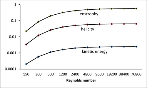
Illustrating the numerical stability and robustness of the Navier-Stokes solver, the next figures present the evolution of the fluctuation parameters and of the correlations of the transport equations as the Reynolds number varies from Re = 150 to Re = 76,800, for the $240\times 60\times 60$ mesh, node 4, with linear UNIFAES discretizations. The mesh does not support reliable Richardson extrapolations for Re = 600 or higher; the unbalances of the transport equations remain as indexes of accuracy.

Figure 3 shows the scalars kinetic energy, helicity and enstrophy sharing almost parallel growth with the Reynolds number: a quick initial increase as the dumping effect of viscosity reduces, tending to stabilize as the flow becomes inviscid. A closer look shows slight growth of the relative distance between the scalars with the increased Reynolds number.

Figure 3. Evolution of scalar properties kinetic energy, modulus of helicity and enstrophy by linear generalized UNIFAES for varying Reynolds number in node 4.

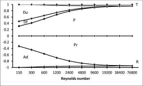
The next figures express the relative magnitudes of the terms of the transport equations, disposed cumulatively. Each term is defined by an area, bounded by curves, whose hight at each Reynolds number is proportional to the magnitude of the term in the balance. Each term is placed above or below depending on its numerical sign if it were on the left member of the equation. Unbalances or residuals (R) are included, growing for crescent Reynolds numbers up to 5.7% of the greatest term for kinetic energy; 6.2%, for helicity; and 14.2%, for enstrophy.

Figure 4 refers to kinetic energy Equation(43) $$\frac{\partial U_j\overline{u_i{u}_i}/2}{\partial x_j}-\nu \frac{{\partial }^2{\overline{u_{i}u}}_i/2}{\partial x_j\partial x_j}=-\overline{u_i{u}_j}{S}_{ij}\mathrm{ }–\frac{\partial \overline{u_{j}p}}{\partial x_j}-\frac{\partial \overline{u_j{u}_i{u}_i}/2}{\partial x_j}\mathrm{ }-\nu \overline{\frac{\partial u_i}{\partial x_j}\frac{\partial u_i}{\partial x_j}}$$(43) (43(43) $$\frac{\partial U_j\overline{u_i{u}_i}/2}{\partial x_j}-\nu \frac{{\partial }^2{\overline{u_{i}u}}_i/2}{\partial x_j\partial x_j}=-\overline{u_i{u}_j}{S}_{ij}\mathrm{ }–\frac{\partial \overline{u_{j}p}}{\partial x_j}-\frac{\partial \overline{u_j{u}_i{u}_i}/2}{\partial x_j}\mathrm{ }-\nu \overline{\frac{\partial u_i}{\partial x_j}\frac{\partial u_i}{\partial x_j}}$$(43) )(43) $$\frac{\partial U_j\overline{u_i{u}_i}/2}{\partial x_j}-\nu \frac{{\partial }^2{\overline{u_{i}u}}_i/2}{\partial x_j\partial x_j}=-\overline{u_i{u}_j}{S}_{ij}\mathrm{ }–\frac{\partial \overline{u_{j}p}}{\partial x_j}-\frac{\partial \overline{u_j{u}_i{u}_i}/2}{\partial x_j}\mathrm{ }-\nu \overline{\frac{\partial u_i}{\partial x_j}\frac{\partial u_i}{\partial x_j}}$$(43) . Production is counterbalanced by the pressure term in the whole spectrum, and these terms dominate at high Reynolds numbers, whilst advection is counterbalanced by diffusion, dissipation and turbulent transport, all of which tend to vanish with growing Reynolds numbers.

Figure 4. Evolution of the relative magnitudes of the terms in the balance of the kinetic energy Equation(43) $$\frac{\partial U_j\overline{u_i{u}_i}/2}{\partial x_j}-\nu \frac{{\partial }^2{\overline{u_{i}u}}_i/2}{\partial x_j\partial x_j}=-\overline{u_i{u}_j}{S}_{ij}\mathrm{ }–\frac{\partial \overline{u_{j}p}}{\partial x_j}-\frac{\partial \overline{u_j{u}_i{u}_i}/2}{\partial x_j}\mathrm{ }-\nu \overline{\frac{\partial u_i}{\partial x_j}\frac{\partial u_i}{\partial x_j}}$$(43) (43(43) $$\frac{\partial U_j\overline{u_i{u}_i}/2}{\partial x_j}-\nu \frac{{\partial }^2{\overline{u_{i}u}}_i/2}{\partial x_j\partial x_j}=-\overline{u_i{u}_j}{S}_{ij}\mathrm{ }–\frac{\partial \overline{u_{j}p}}{\partial x_j}-\frac{\partial \overline{u_j{u}_i{u}_i}/2}{\partial x_j}\mathrm{ }-\nu \overline{\frac{\partial u_i}{\partial x_j}\frac{\partial u_i}{\partial x_j}}$$(43) )(43) $$\frac{\partial U_j\overline{u_i{u}_i}/2}{\partial x_j}-\nu \frac{{\partial }^2{\overline{u_{i}u}}_i/2}{\partial x_j\partial x_j}=-\overline{u_i{u}_j}{S}_{ij}\mathrm{ }–\frac{\partial \overline{u_{j}p}}{\partial x_j}-\frac{\partial \overline{u_j{u}_i{u}_i}/2}{\partial x_j}\mathrm{ }-\nu \overline{\frac{\partial u_i}{\partial x_j}\frac{\partial u_i}{\partial x_j}}$$(43) for varying Reynolds number, node 4, $240\times 60\times 60$ mesh, linear generalized UNIFAES.

For helicity and enstrophy equations, Figures 5 and 6, the net advection terms change their signs as the Reynolds number grows. A simple one-dimensional explanation exists for enstrophy: negative advection at node 4 for the low Reynolds numbers corresponds to decrease of enstrophy downwind, as observed between nodes 4 and 13 for Re = 300 (Table 1), whilst positive advection for the high Reynolds number implies enstrophy increase, as seen between the same nodes for Re = 9,600 (Table 2). Such one-dimensional explanation does not hold for helicity, whose modulus decreases from node 4 to node 13 for both Re = 300 and Re = 9,600; in this case the reversed advection is possibly in spanwise direction, considering the deformed mean velocity field at node 4 for Re = 9,600: $U_i=(0.5088, 0.0002, 0.0219).$

Figure 5. Evolution of the relative magnitudes of the terms in the balance of the helicity Equation(45) $$\frac{\partial \overline{u_i{w}_i}{U}_j}{\partial x_j}-\nu \frac{{\partial }^2\overline{{u_{i}w}_i}}{\partial x_j\partial x_j}={\overline{\frac{\partial u_i{u}_j}{\partial x_j}}W}_i-\overline{u_i{u}_j}\frac{\partial W_i}{\partial x_j}-\overline{w_i\frac{\partial p}{\partial x_i}}+\overline{u_i{w}_j{s}_{ij}}-\frac{\partial \overline{u_i{w}_i{u}_j}}{\partial x_j}-2\nu \overline{\frac{\partial u_i}{\partial x_j}\frac{\partial w_i}{\partial x_j}}$$(45) (45(45) $$\frac{\partial \overline{u_i{w}_i}{U}_j}{\partial x_j}-\nu \frac{{\partial }^2\overline{{u_{i}w}_i}}{\partial x_j\partial x_j}={\overline{\frac{\partial u_i{u}_j}{\partial x_j}}W}_i-\overline{u_i{u}_j}\frac{\partial W_i}{\partial x_j}-\overline{w_i\frac{\partial p}{\partial x_i}}+\overline{u_i{w}_j{s}_{ij}}-\frac{\partial \overline{u_i{w}_i{u}_j}}{\partial x_j}-2\nu \overline{\frac{\partial u_i}{\partial x_j}\frac{\partial w_i}{\partial x_j}}$$(45) )(45) $$\frac{\partial \overline{u_i{w}_i}{U}_j}{\partial x_j}-\nu \frac{{\partial }^2\overline{{u_{i}w}_i}}{\partial x_j\partial x_j}={\overline{\frac{\partial u_i{u}_j}{\partial x_j}}W}_i-\overline{u_i{u}_j}\frac{\partial W_i}{\partial x_j}-\overline{w_i\frac{\partial p}{\partial x_i}}+\overline{u_i{w}_j{s}_{ij}}-\frac{\partial \overline{u_i{w}_i{u}_j}}{\partial x_j}-2\nu \overline{\frac{\partial u_i}{\partial x_j}\frac{\partial w_i}{\partial x_j}}$$(45) for varying Reynolds number, node 4, $240\times 60\times 60$ mesh, linear generalized UNIFAES.

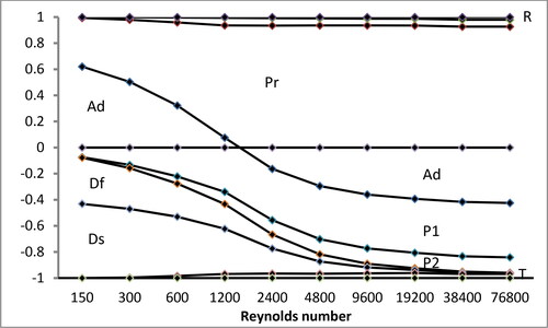
Figure 6. Evolution of the relative magnitudes of the terms in the balance of the enstrophy Equation(46) $$\frac{\partial U_j\overline{w_i{w}_i/2}}{\partial x_j}-\upsilon \frac{{\partial }^2\overline{{w_{i}w}_i}/2}{\partial x_j\partial x_j}=\overline{w_i{s}_{ij}}{W}_j+\overline{w_i{w}_j}{S}_{ij}-\overline{w_i{u}_j}\frac{\partial W_i}{\partial x_j}-\frac{\partial \overline{u_j{w}_i{w}_i/2}}{\partial x_j}\text{-}\mathrm{ }\overline{w_i{w}_j{s}_{ij}}\mathrm{ }-\upsilon \overline{\frac{\partial w_i}{\partial x_j}\frac{\partial w_i}{\partial x_j}}$$(46) (46(46) $$\frac{\partial U_j\overline{w_i{w}_i/2}}{\partial x_j}-\upsilon \frac{{\partial }^2\overline{{w_{i}w}_i}/2}{\partial x_j\partial x_j}=\overline{w_i{s}_{ij}}{W}_j+\overline{w_i{w}_j}{S}_{ij}-\overline{w_i{u}_j}\frac{\partial W_i}{\partial x_j}-\frac{\partial \overline{u_j{w}_i{w}_i/2}}{\partial x_j}\text{-}\mathrm{ }\overline{w_i{w}_j{s}_{ij}}\mathrm{ }-\upsilon \overline{\frac{\partial w_i}{\partial x_j}\frac{\partial w_i}{\partial x_j}}$$(46) )(46) $$\frac{\partial U_j\overline{w_i{w}_i/2}}{\partial x_j}-\upsilon \frac{{\partial }^2\overline{{w_{i}w}_i}/2}{\partial x_j\partial x_j}=\overline{w_i{s}_{ij}}{W}_j+\overline{w_i{w}_j}{S}_{ij}-\overline{w_i{u}_j}\frac{\partial W_i}{\partial x_j}-\frac{\partial \overline{u_j{w}_i{w}_i/2}}{\partial x_j}\text{-}\mathrm{ }\overline{w_i{w}_j{s}_{ij}}\mathrm{ }-\upsilon \overline{\frac{\partial w_i}{\partial x_j}\frac{\partial w_i}{\partial x_j}}$$(46) for varying Reynolds number, node 4, $240\times 60\times 60$ mesh, linear generalized UNIFAES.

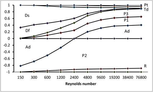
In the helicity equation, the pressure term counterbalances all other terms for Re $\cong$1,500 or greater. In the enstrophy equation, the production term P2, associated to the mean shear rate, counterbalances all other terms for Re $\cong$2,400 or greater. The viscous terms diffusion and dissipation of both helicity and enstrophy vanish as the Reynolds number grows, whilst mean and turbulent advection and production terms tend to stabilize.

Conclusion

The UNIFAES discretization scheme, originally restrict to the combined advective and viscous fluxes, has been generalized to most terms of complex transport equations by turning the first and second order derivatives, which are implicit in its interpolating curve, explicit. By construction, the UNIFAES differences are non-linear approximations to linear derivatives; a linear approximation to generalized UNIFAES was defined for steady mean flows by using the local mean velocity field as reference for all derivations.

The restrict scheme was applied to a Navier Stokes solver, and the generalized scheme was applied, alongside central differencing schemes, for processing statistical correlations of the transport equations for fluctuating kinetic energy, helicity, and enstrophy in a perturbed laminar Coutte flow.

Linear and non-linear UNIFAES discretizations produced very close results for helicity and enstrophy for low Reynolds number, and moderately distinct values for high Reynolds number.

This problem hinders the direct comparison of the accuracy of the schemes for measuring the correlations because results depend primarily on the solver, but an indirect comparison emerged. In most cases, for both high and low Reynolds numbers, the results of helicity and enstrophy with generalized UNIFAES, both linear and nonlinear, were closer to the fourth order central differencing than to the second order.

Deterioration of precision was expected as correlations gained complexity, involving up to third order velocity derivatives in the viscous terms of vorticity. However, the statistics of the transport equations for kinetic energy, helicity and enstrophy for Re = 300 were shown to converge with asymptotic second order, with higher order terms of the error still relevant in the meshes used. In the referred literature on the restrict UNIFAES in steady-state problems, second order dominated solutions were found at higher Reynolds numbers, with comparable mesh refinement. So, the expected deterioration of precision appears to manifest as precocious loss of dominance of second order terms of the error, not as decreased order of convergence.

Acknowledgements

The author thanks Espaço da Escrita – Pró-Reitoria de Pesquisa – UNICAMP for the language services provided.

References

- R. F. Warming and R. M. Beam, “Upwind second-order difference scheme and applications in aerodynamics flows,” AIAA Journal, vol. 14, no. 9, pp. 1241–1249, 1976. DOI: 10.2514/3.61457.
- B. Leonard, “A stable and accurate convective modeling procedure based on quadratic upstream interpolation,” Computer Methods APPl. Mechanics Engineering, vol. 19, no. 1, pp. 59–98, 1979. DOI: 10.1016/0045-7825(79)90034-3.
- S. V. Patankar, Numerical Heat Transfer and Fluid Flow. New York, NY: hemisphere Publ. Corp., 1980,
- J. R. Figueiredo, “A unified finite-volume finite-differencing exponential-type scheme for the convective-diffusive fluid transport equations,” J. Braz. Society Mech. Sciences, vol. 19, no. 3, pp. 371–391, 1997.
- J. R. Figueiredo and J. Llagostera, “Comparative study of the unified finite approach exponential-type scheme (UNIFAES) and its application to natural convection in a porous cavity,” Numerical Heat Transfer, B, vol. 35, no. 3, pp. 347–367, 1999. DOI: 10.1080/104077999275901.
- J. Llagostera and J. R. Figueiredo, “Application of the UNIFAES discretization scheme to mixed convection in a porous layer with cavity, using the Darcy model,” J Por Media, vol. 3, no. 2, pp. 16, 2000. DOI: 10.1615/JPorMedia.v3.i2.40.
- J. Llagostera and J. R. Figueiredo, “Numerical study on mixed convection in a horizontal flow past a square cavity using UNIFAES scheme,” J. Braz. Soc. Mech. Sci, vol. 22, no. 4, pp. 583–597, 2000. DOI: 10.1590/S0100-73862000000400008.
- J. R. Figueiredo and K. P. M. Oliveira, “Comparative study of UNIFAES and other finite-volume schemes for the discretization of advective and viscous fluxes in incompressible Navier-Stokes equations, using various mesh structures,” Numerical Heat Transfer, B, vol. 55, no. 5, pp. 406–434, 2009. DOI: 10.1080/104077909027766.
- J. R. Figueiredo and K. P. M. Oliveira, “Comparative study of the accuracy of the fundamental mesh structures for the numerical solution of incompressible Navier-Stokes equations in the two-dimensional cavity problem,” Numerical Heat Transfer, B, vol. 55, no. 5, pp. 406–434, 2009. DOI: 10.1080/10407790902779978.
- A. H. G. Nascimento, G. S. Rodrigues and J. R. Figueiredo, “Incompressible Flows Bifurcation Phenomena in Symmetric Channels,” In Proc. 25th ABCM Intern. Congress of Mech. Eng., Uberlândia, 2019.
- G. S. Rodrigues, A. H. G. Nascimento and J. R. Figueiredo, “Performance of finite volume discretization schemes in the backward-facing step problem—part I: stability of schemes,” In Proc. 25th ABCM Intern. Congress of Mech. Eng., Uberlândia, 2019. DOI: 10.26678/abcm.cobem2019.cob2019-032328.
- G. S. Rodrigues, A. H. G. Nascimento and J. R. Figueiredo, “Performance of finite volume discretization schemes in the backward facing step problem—part II: numerical error of schemes,” In Proc. 25th ABCM Intern. Congress of Mech. Eng., Uberlândia, 2019. DOI: 10.26678/abcm.cobem20.19.cob2019-0324
- G. S. Rodrigues, A. H. G. Nascimento and J. R. Figueiredo, “Numerical assessment of finite volume schemes for incompressible viscous flows on non-staggered meshes,” J Braz. Soc. Mech. Sci. Eng, vol. 43, no. 12, pp. 564, 2021. DOI: 10.1007/s40430-021-03268-y.
- R. G. Santos and J. R. Figueiredo, “Numerical simulation study in a three-dimensional backward-facing step flow,” 21st International Congress of Mechanical Engineering, Natal, RN, 2011.
- A. Nascimento, G. Rodrigues and J. R. Figueiredo, “A semi-staggered finite volume approach applied to two- and three-dimensional flow in channels with gradual expansions,” Int J Numer Meth Fluids, vol. 93, no. 10, pp. 3053–3072, 2021. DOI: 10.1002/fld.5024.
- H. Tennekes and J. L. Lumley, A First Course in Turbulence. Cambridge, MA: MIT Press, 1972,
- H. K. Moffatt and A. Tsinober, “Helicity in laminar and turbulent flow,” Annu. Rev. Fluid Mech, vol. 24, no. 1, pp. 281–312, 1992. DOI: 10.1146/annurev.fl.24.010192.001433.
- D. D. Holm and R. M. Kerr, “Helicity in the formation of turbulence,” Physics Fluids, vol. 19, no. 2, pp. 025101, 2007. DOI: 10.1063/1.2375077.
- V. Dallas and S. M. Tobias, “Forcing-dependent dynamics and emergence of helicity in rotating turbulence,” J. Fluid Mech, vol. 798, pp. 682–695, 2016. DOI: 10.1017/jfm.2016.341.
- Z. Yan, X. Li and C. Yu, “Scale locality of helicity cascade in physical space,” Phys. Fluids, vol. 32, no. 6, pp. 061705, 2020. DOI: 10.1063/5.0013009.
- T. A. Oliver, N. Malaya, R. Ulerich and R. D. Moser, “Estimating uncertainties in statistical category computed from direct numerical simulations,” Phys. Fluids, vol. 26, no. 3, pp. 035101, 2014. DOI: 10.1063/1.486683.
- J. R. Andrade, R. S. Martins, R. L. Thompson, G. Mompean, A. and Silveira, Neto, “Analysis of uncertainties and convergence of the statistical quantities in turbulent wall-bounded flows by means of a physically based criterion,” Physics of Fluids, vol. 30, no. 4, pp. 045106, 2018. DOI: 10.1063/1.5023500.
- D. N. G. Allen and R. V. Southwell, “Relaxation Methods Applied to Determine the Motion, in Two Dimensions, of a Viscous Flow Past a Fixed Cylinder,” Q J Mechanics Appl Math, vol. 8, no. 2, pp. 129–145, 1955. DOI: 10.1093/qjmam/8.2.129.
- H. H. Wong and G. D. Raithby, “Improved Finite-Difference Methods Based on a Critical Evaluation of the Approximation Errors,” Numer. Heat Transfer. vol, vol. 2, no. 2, pp. 139–163, 1979. DOI: 10.1080/10407787908913404.
- C. Prakash, “Application of the Locally Analytic Differencing Scheme to Some Test problems for the Convection-Diffusion Equation,” Numer. Heat Transfer, vol. 7, no. 2, pp. 165–182, 1984. DOI: 10.1080/01495728408961818.
- L. M. C. Varejão, “Flux-Spline Method for Heat and Momentum Transfer,” Ph. D. Thesis, University of Minnesota, 1979., Minneapolis,
- K. C. Karki, S. V. Patankar and H. C. Mongia, “Three-dimensional fluid flow calculations using a flux-spline method,” Aiaa J, vol. 28, no. 4, pp. 631–634, April 1990.
- P. C. Oliveira, “Flux-spline scheme applied to open cavities with natural convection” (in Portuguese), Doctoral Thesis, School of Mechanical Engineering, Campinas State University, Campinas, SP, Brazil,” 1997.
- B. Kuznetsov, “Numerical methods for solving problems of fluid flow,” Fluid Dynamics Transactions, vol. 4, pp. 85–89, 1968.
- R. Peyret and T. D. Taylor, Computational Methods for Fluid Flow, 2nd ed. New York: Springer-Verlag, 1983.
- J. R. Figueiredo and K. P. M. Oliveira, “Reevaluation of the Vertex Collocated Mesh for Primitive Variable Computation of Incompressible Fluid Flows by Enforcing Continuity-Based Conditions,” Numerical Heat Transfer, B, vol. 60, no. 3, pp. 168–178, 2011.
- C. M. Rhie and L. Chow, “Numerical study of the turbulent flow past an airfoil with trailing edge separation,” AIAA Journal, vol. 21, no. 11, pp. 1525–1532, 1983. DOI: 10.2514/3.8284.
- B. E. Launder and D. B. Spalding, Mathematical Models of Turbulence, London: academic Press, 1972,
- P. R. Spalart, “Philosophies and fallacies in turbulence modeling,” Progress Aerospace Sciences, vol. 74, pp. 1–15, 2015. DOI: 10.1016/paerosci.2014.12.004.
- T. B. Gatski, “Constitutive equations for turbulent flows,” Theor. Comput. Fluid Dyn, vol. 18, no. 5, pp. 345–369, 2004. DOI: 10.1007/s00162-004-0119-3.
- K. Hanjalic, “Advanced turbulence closure models: a view of current status and future prospects,” Int. J. Heat Fluid Flow, vol. 15, no. 3, pp. 178–203, 1994.
- C. D. Argyropoulos and N. C. Markatos, “Recent advances on the numerical modeling of turbulent flows,” APPl. Math. Modeling, vol. 39, no. 2, pp. 693–732, 2015. NC, DOI: 10.1016/j.apm.2014.07.001.
- J. O. Hinze, Turbulence. New York, NY: McGraw-Hill, 1959.