A two-level machine learning approach for predicting thermal striping in T-junctions with upstream elbow

Abstract

Thermal striping is a phenomenon characterized by oscillatory mixing of non-isothermal streams, which is commonly seen in industrial processes such as nuclear coolant piping, petrochemical plants and liquefied natural gas transportation. The oscillatory mixing of hot and cold fluid can produce thermal field fluctuations and pose a potential risk of high-cycle thermal fatigue failures. Predicting and evaluating spatiotemporal fluctuations in thermal striping often requires high resolution and massive computational power. Although there have been extensive studies using machine learning algorithms on surrogate modeling, research focused on spatiotemporal fluctuation predictions is very limited. Due to the high dimensionality, it often requires complex algorithms with a large amount of high-fidelity training data, which limits the adoption of such methods for industrial applications. In this research, a two-level machine learning framework based on turbulence coherent structures is proposed and its application to a practical problem is demonstrated. The two-level design leverages vortex identification and local bias correction techniques, efficiently reducing the number of full-order simulations required for training. In the first level, well-organized coherent structures are extracted by performing Proper Orthogonal Decomposition on local parameters and then a tree-based machine-learning model is used to down-select the reference structures for the field reconstruction. In the second level, a parameterized convolution neural network is trained to predict the bias introduced by reference structures approximation. The demonstration of the methodology shows that the method can accurately capture the fluctuation frequencies and amplitudes of the spatiotemporal fields in a highly variational setting. Based on the vortex identification method, the methodology is expected to be applicable to general phenomenon driven by large coherent structures.

Keywords:

• Machine learning
• surrogate modeling
• thermal striping
• turbulent structures

1. Introduction

Thermal striping is a phenomenon in which incomplete fluid stream mixing at different temperatures results in random thermal fluctuations. It is known to be one of the major concerns for high-cycle thermal fatigue in nuclear piping systems. The phenomenon was initially studied in liquid-metal fast breeder reactors (LMFBRs) [1–3] and has gained increased attention in light-water reactors, as several occurrences of fatigue failure have been reported [4–6]. Beyond nuclear industries, mixing process in T-junctions is an industrial piping feature commonly seen in heating, ventilation and air conditioning (HVAC) systems [7], liquefied natural gas (LNG) transportation [8], and exhaust gas recirculation in combustion engines [9].

In nuclear piping systems, this phenomenon is not easily monitored by in-plant instrumentations due to the involvement of complex turbulence flow and operation of piping systems at high temperatures and high pressure. Simulation and model-based prognostic tools are essential for evaluating and predicting the high-cycle thermal fatigue induced by thermal striping. Computational fluid dynamics (CFD) coupled with finite-element analysis (FEA) provide high resolution for this multi-physics problem. However, the problem complexity makes the computational cost overly burdensome, which limits the exploration of multi-query applications such as digital twin technologies and design iterations.

Several synthetic methods, such as the sinusoidal method (SIN) [6, 10], random thermal load spectrums [11, 12], and synthetic temperature spectrums [13, 14], have been proposed to reduce the computational cost. However, thermal striping is a three-dimensional phenomenon that exhibits high degree of variability under parametric variations, for both affected locations and critical frequencies [15–17]. These methods are unable to effectively address this challenge as: (1)(1) $${\mathit{u}}_h\left(t;\mathit{\mu }\right)\approx {\widehat{\mathit{u}}}_h\left(t;\mathit{\mu }\right)=\sum _{m=0}^r{\mathit{\varphi }}_m{\mathrm{ }\left(\mathit{\mu }\right)a}_m\left(t;\mathit{\mu }\right)$$(1) they extensively rely on pre-determined frequencies/power spectrums density (PSD) from mockup experiments or high-fidelity simulations, and (2)(2) $${\mathit{S}}^{\left(k\right)}=\left[{\mathit{u}}_{\mathit{h}}\left(t_1;{\mathit{\mu }}^{\left(k\right)}\right)\left|{\mathit{u}}_{\mathit{h}}\right(t_2;{\mathit{\mu }}^{\left(k\right)}\left)\right|\cdots \left|{\mathit{u}}_{\mathit{h}}\right(t_{N_t};{\mathit{\mu }}^{\left(k\right)})\right]$$(2) they are often based on substantial simplifications and assumptions, such as assuming sinusoidal behavior and isotropic turbulence. Prognostic tools that are able to address variations in critical frequencies and fatigue locations are also lacking. There is a strong need to reduce the computational cost of thermal striping evaluations under parametric variations.

This study aims to construct a parametric thermal striping surrogate which relies on limited queries of expensive full-order simulations. We apply a novel two-level machine learning framework under parametric settings. The proposed framework is non-intrusive, i.e. purely based on the data obtained from experiments or simulations. A T-junction with a bent pipe connected upstream, a commonly seen configuration in nuclear piping systems, is selected for demonstration. CFD simulations based on the STRUCTure-based (STRUCT) turbulence modeling approach [18, 19] are used to generate the data for ML algorithm training. In this article, we focus on the root cause of the thermal field fluctuations—the spatial-temporal relations of turbulence mixing, which is vital to a successful prediction of the thermal field variations. Results assessed against the velocity field fluctuations are presented and discussed.

The article is structured as follows: Section 2 describes the geometry and the numerical setup of the full-order simulations; Section 3 details the methodology and the training database used for the development of the framework. The results of the fluid field spatiotemporal fluctuations and the solid stress emulation are present in Section 4. The summary and conclusion of the current work are presented in Section 5.

2. Numerical setup

In this work, we consider a T-junction with a 90° bend upstream, as illustrated in Figure 1. In this configuration, hot water coming from the branch pipe is mixed with the cold fluid from the main pipe. Two convergent flows with different temperature are mixed at the junction area. The horizontal main pipe has 90° bend $2D_m$ upstream of the junction, with a radius of curvature $R_c=1.4D_m.$ The configuration is tabulated in Table 1. Fully-developed turbulent conditions are assumed at both inlets. Water is chosen as the working fluid.

Figure 1. Schematic of the T-junction flow configuration with upstream elbow.

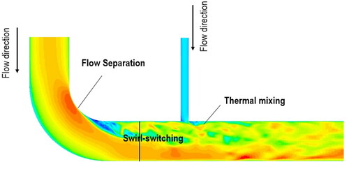
Table 1. The geometry of the elbow tee configuration.

	Main	Branch
Mass flow rate ($\mathit{\text{kg}}/s)$	${\dot{m}}_c=$63.32 ∼ 601.3	${\dot{m}}_h=$0.65 ∼ 5.65
Temperature ($\mathrm{°C})$	$T_c=$40	$T_h=$240
Diameter (mm)	$D_m=$387.35	$D_b=$49.48
Elbow radius of curvature (mm)	$R_c=$542.29
Distance between bend and junction (mm)	$L=$774.7

Upon entering the pipe bend, a strong adverse pressure gradient builds up, causing flow separation and the development of secondary flow patterns consisting of swirling regions of fluid. Downstream of the bend, a pair of counter-rotating vortices, known as Dean vortices, can be observed [20, 21]. These vortices are typically found to be present in bi-stable states with low oscillatory frequencies, where one vortex alternatively dominates over the other, a phenomenon known as swirl-switching [22–24]. Moving further downstream, the hot water pumped into the branch line interacts with the bulk flow, leading to the formation of a shear layer and turbulence mixing near the junction, as depicted in Figure 1.

The high-fidelity simulations in this study are based on the STRUCT (Structure-based resolution of turbulence) turbulence model. This hybrid turbulence approach was proposed by Lenci [18, 19], and later reformulated by Xu [25], and is designed to enhance the URANS approach by providing local resolution of turbulent structures. The model has been validated against LES and experimental data for application to thermal striping, demonstrating high accuracy, with an order of 100 reduction in the computational cost in comparison to LES requirements [26, 27]. The simulations discussed in this work are performed with the commercially available STAR-CCM + ver.15.06 software. The SIMPLE [28] based segregated flow solver is adopted in conjunction with second-order non-oscillatory treatment for advective terms as well as implicit second order time integration.

3. Data-driven thermal striping emulator using turbulence coherent structures

Unlike the traditional framework of the reduced basis (RB) method, which attempts to construct a parametric-independent reduced space, the proposed approach takes a distinct viewpoint. Instead of constructing a reduced space, the framework aims at achieving two key objectives: (1)(1) $${\mathit{u}}_h\left(t;\mathit{\mu }\right)\approx {\widehat{\mathit{u}}}_h\left(t;\mathit{\mu }\right)=\sum _{m=0}^r{\mathit{\varphi }}_m{\mathrm{ }\left(\mathit{\mu }\right)a}_m\left(t;\mathit{\mu }\right)$$(1) identifying the dominating flow eddies and their spatial-temporal relations in the flow (2)(2) $${\mathit{S}}^{\left(k\right)}=\left[{\mathit{u}}_{\mathit{h}}\left(t_1;{\mathit{\mu }}^{\left(k\right)}\right)\left|{\mathit{u}}_{\mathit{h}}\right(t_2;{\mathit{\mu }}^{\left(k\right)}\left)\right|\cdots \left|{\mathit{u}}_{\mathit{h}}\right(t_{N_t};{\mathit{\mu }}^{\left(k\right)})\right]$$(2) utilizing machine learning algorithms to predict the parametric dependency of the eddies and emulate their motions.

It is assumed that the velocity and temperature solutions from high-fidelity simulations can be decomposed in the following form: (1) $${\mathit{u}}_h\left(t;\mathit{\mu }\right)\approx {\widehat{\mathit{u}}}_h\left(t;\mathit{\mu }\right)=\sum _{m=0}^r{\mathit{\varphi }}_m{\mathrm{ }\left(\mathit{\mu }\right)a}_m\left(t;\mathit{\mu }\right)$$(1) here ${\mathit{u}}_{\mathit{h}}\in {\mathbb{R}}^{N_x}$ and represents the field observables with input boundary conditions $\mathit{\mu };$ ${\varphi }_m(\mathit{\mu })$ and is the spatial basis functions and $a_m(t;\mathit{\mu })$ is the temporal coefficients; where $r$ is the number of modes for approximation. In this work, we leverage the concept of turbulence coherent structures to choose physically meaningful spatial functions, ${\varphi }_m\left(\mathit{x};\mathit{\mu }\right)$ for a given parametric configurations.

3.1. Parametric-dependent spatial basis: Turbulence coherent structures

Turbulence coherent structures, often loosely defined as “vortices”, are the fundamental feature of turbulent fluid flows that show a degree of organization within a seemingly chaotic system. Extensive research has observed that organized motions, involving distinct energy scales, exist in localized regions where the spatiotemporal field exhibits characteristic coherent patterns [29–31].

Numerous attempts have been made to develop quantitative descriptions of turbulence. In 1967, Lumley adopted the modal decomposition method using proper orthogonal decomposition (POD) to identify the low-order dynamics of turbulence flow [32]. Such methods describe the fluid state as a superposition of empirically computed basis vectors, or “modes. The method has been widely applied on flow diagnostics to understand the relations between motion, forces, and energy. It is shown that POD can successfully identify the high-energy spatial structures and dominating frequencies in jets [33], pipe bends [34], crossflow [35], and T-junctions [24], among others.

In this work, the parameter-dependent coherent structures are extracted from the solutions of CFD simulations. A local proper orthogonal decomposition (LPOD) technique is used. The term “local POD” refers to extracting coherent structures at a local parametric configuration. Unlike the standard (globally parametric-independent) POD utilized in the reduced-basis methods, the local POD provides a diagnostic view of turbulence, revealing the most active vortices present in the flow.

Given a sample of input parameter ${\mathit{\mu }}^{(k)},$ the solutions from high-fidelity simulations can be collected as a snapshot matrix: (2) $${\mathit{S}}^{\left(k\right)}=\left[{\mathit{u}}_{\mathit{h}}\left(t_1;{\mathit{\mu }}^{\left(k\right)}\right)\left|{\mathit{u}}_{\mathit{h}}\right(t_2;{\mathit{\mu }}^{\left(k\right)}\left)\right|\cdots \left|{\mathit{u}}_{\mathit{h}}\right(t_{N_t};{\mathit{\mu }}^{\left(k\right)})\right]$$(2)

The POD modes can be computed through Singular Value Decomposition (SVD): (3) $${\mathit{S}}^{\left(k\right)}={\mathit{U}}^{\left(k\right)}{\mathbf{\Sigma }}^{\left(k\right)}{\mathit{V}}^{\left(k\right)}$$(3)

The column vectors of ${\mathit{U}}^{(k)}$ are the identified spatial mode, i.e. coherent structures ${\mathit{\varphi }}_m\left({\mathit{\mu }}^{\left(k\right)}\right),$ for a given parametric setting. The temporal coefficient for this mode can be found as ${\mathit{a}}_m^{(k)}={\sigma }_m^{(k)}{\mathit{v}}_m^{(k)},$ where ${\sigma }_m^{(k)}$ is the $m^{\mathit{\text{th}}}$ singular value in ${\mathbf{\Sigma }}^{(k)}$ and ${\mathit{v}}_m^{(k)}$ is the $m^{\mathit{\text{th}}}$ row vector of the ${\mathit{V}}^{(k)}.$

In the pre-processing stage, each structure in the library is converted into three descriptors to represent the structure characteristics:

1. Spatial descriptor (${\rho }_m$): as the spatial modes give the topological information of the turbulence coherent structures, this metric is used to evaluate the size of the active fluctuation region, i.e., the size of the spatial mode where the value is greater than a tolerance value $ϵ.$

(4) $${\rho }_m=\sum _{i=1}^{N_x}1\left({\mathit{x}}_i\right)$$(4) here $1\left({\mathit{x}}_i\right)$ is the indicator function, defined as (5) $$1\left({\mathit{x}}_i\right)=\{\begin{array}{c}1 \\ 0\end{array}\mathrm{ }\begin{array}{c}\mathrm{ }\mathit{\text{if}}\mathrm{ }\left|{\varphi }_j\left({\mathit{x}}_i\right)\right|>ϵ\\ e\mathit{\text{lse}}\end{array}$$(5)

A tolerance value $ϵ=1\times {10}^{-5}$ is adopted.

• Temporal descriptor (${\mathit{\nu }}_{\mathit{m}}$): the temporal coefficients describe the fluctuating behavior of the coherent structures (i.e., moving fast or slow). For each structure, the temporal coefficients are converted into a power spectrum density (PSD). The frequency corresponding to the maximum PSD peak is recorded as the dominant mode frequency ${\nu }_m.$

• Energy descriptor (${\mathit{\sigma }}_{\mathit{m}}^{\mathit{*}}$): the singular values ($\sigma$) from SVD indicate the ranking of the structures based on their contribution to the total energy. The singular values ${\mathbf{\Sigma }}^{(k)}\mathit{ }$ signifies the contribution of each low-rank component to the total variation of the original matrix, which can be seen as the amount of energy preserved in each mode. The metric is defined as: (6) $${\sigma }_m^{\mathrm{*}}=\frac{{\sigma }_m}{\sum _{j=1}^r{\sigma }_j}$$(6)

3.2. Predicting the coherent structures: a two-level machine learning framework

In thermal striping applications, there exists a strong nonlinear relationship between input parameters and turbulence structures. Although machine learning algorithms are powerful tools in treating nonlinearity in high-dimensional space, they often require a large amount of training data to achieve reliable performance. To overcome this limitation, the present work adopts a selection-correction scheme to improve the data efficiency. Notably, the approach is synthetic, meaning that the surrogate method aims to emulate the system response with the same oscillatory behavior, rather than matching the time history of the flow oscillation. This is because high-cycle thermal fatigue is evaluated at quasi-steady state operational conditions. In practice, the time-history of measurements or simulations may be obtained from different time steps. Therefore, it is appropriate to focus on the quasi-steady state characterizes that are more relevant to high-cycle thermal fatigue evaluations.

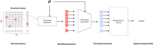
The framework consists of three components: (1)(1) $${\mathit{u}}_h\left(t;\mathit{\mu }\right)\approx {\widehat{\mathit{u}}}_h\left(t;\mathit{\mu }\right)=\sum _{m=0}^r{\mathit{\varphi }}_m{\mathrm{ }\left(\mathit{\mu }\right)a}_m\left(t;\mathit{\mu }\right)$$(1) structure library, (2)(2) $${\mathit{S}}^{\left(k\right)}=\left[{\mathit{u}}_{\mathit{h}}\left(t_1;{\mathit{\mu }}^{\left(k\right)}\right)\left|{\mathit{u}}_{\mathit{h}}\right(t_2;{\mathit{\mu }}^{\left(k\right)}\left)\right|\cdots \left|{\mathit{u}}_{\mathit{h}}\right(t_{N_t};{\mathit{\mu }}^{\left(k\right)})\right]$$(2) structure predictor (3)(3) $${\mathit{S}}^{\left(k\right)}={\mathit{U}}^{\left(k\right)}{\mathbf{\Sigma }}^{\left(k\right)}{\mathit{V}}^{\left(k\right)}$$(3) structure corrector. The framework construction is summarized below; the detailed framework descriptions can be found in the reference [36].

Library construction

Given the parametric domain $\mathcal{P}$ and the parameter sampling ${\mathcal{P}}_d=\left\{{\mathit{\mu }}^{\left(1\right)},{\mathit{\mu }}^{\left(2\right)},\dots {\mathit{\mu }}^{\left(N_p\right)}\right\}\subset \mathcal{P},$ the high-fidelity solution of each sample parameter is processed by local POD and converted to the structure descriptors, as illustrated in the previous section.

Structure predictor

The parameter-descriptor pairs in the library are used to train a Gradient-Boosting multi-output regressor: (7) $$\left(m,\mathit{\mu }\right)⟼\mathit{\text{GB}}\left(m,\mathit{\mu }\right)=\left({\widehat{\rho }}_m\left(\mathit{\mu }\right),{\widehat{\nu }}_m\left(\mathit{\mu }\right),{\widehat{\rho }}_m^{\mathrm{*}}\left(\mathit{\mu }\right)\right)$$(7)

In the prediction stage, the reference structures are determined by comparing the descriptors in the library and selecting the structures with the lowest $L^2$ norm scores.

Structure corrector

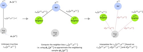
To reduce the bias introduced by library approximation, we train a parameterized Convolutional Neural Network (CNN) to predict the bias using nonlinear interpolation. This approach is particularly useful for detecting the deformation and shifting of coherent structures, which is essential for predicting the behavior of fluid flow. CNNs are well-suited for this task, as they can learn to identify key features and patterns of coherent structures. In the absence of knowledge of the true bias, the idea of nonlinear interpolation is to utilize the information of the approximation error obtained from the neighboring samples, as illustrated in Figure 2. The training procedure is listed below:

Figure 2. Nonlinear interpolation of bias based on parametric distance. For a given mode index $\mathit{m}$ and an input parameter vector $\mathit{\mu },$ the reference mode ${\mathit{\varphi }}_m\left({\mathit{\mu }}^{\left(\mathit{*}\right)}\right)$ is obtained from the structure predictor. The term ${\mathit{ϵ}}_{\mathit{m}}\left(\mathit{\mu },{\mathit{\mu }}^{\left(\mathit{*}\right)}\right)$ is the approximation bias between two different inputs ${\mathit{ϵ}}_{\mathit{m}}\left(\mathit{\mu },{\mathit{\mu }}^{\left(\mathit{*}\right)}\right)={\mathit{\varphi }}_m\left(\mathit{\mu }\right)-{\mathit{\varphi }}_m\left({\mathit{\mu }}^{\left(\mathit{*}\right)}\right);\mathit{d}\left(\mathit{\mu },{\mathit{\mu }}^{\left(\mathit{*}\right)}\right)=\Vert \mathit{\mu }-{\mathit{\mu }}^{\mathit{*}}\Vert$ is the parametric distance.

• For every target sample $\mathit{\mu }$ and the mode index $m,$ the reference spatial mode ${\mathit{\varphi }}_m({\mathit{\mu }}^{*})$ is obtained from the structure predictor. The bias of using ${\mathit{\varphi }}_m({\mathit{\mu }}^{*})$ to approximate ${\mathit{\varphi }}_m(\mathit{\mu })$ is denoted as ${\mathit{ϵ}}_m\left(\mathit{\mu },{\mathit{\mu }}^{*}\right),$ which is assumed to be a function of Euclidean distance between $\mathit{\mu }$ and ${\mathit{\mu }}^{*},$ i.e. $\mathit{d}\left(\mathit{\mu },{\mathit{\mu }}^{\mathit{*}}\right)=\Vert \mathit{\mu }-{\mathit{\mu }}^{*}\Vert .$

• Next, we select $n$ neighboring samples $\{{\mathit{\mu }}^{\left(\mathit{i}\right)}:i\in {\mathcal{N}}_n\}$ near the target as the interpolation references. Here ${\mathcal{N}}_n\subset {\mathcal{P}}_d$ is the neighbor sample set.

• The neighbor biases ${\{\mathit{ϵ}}_{\mathit{m}}\left({\mathit{\mu }}^{\left(\mathit{i}\right)},{\mathit{\mu }}^{\mathit{*}}\right):i\in {\mathcal{N}}_n\}$ and the parametric distance $\left\{\mathit{d}\right({\mathit{\mu }}^{\left(\mathit{i}\right)},{\mathit{\mu }}^{\mathit{*}}):\mathit{i}\in {\mathcal{N}}_{\mathit{n}}\}$ are computed and serve as the inputs of the parameterized CNN.

After obtaining the reference structures and the predicted bias, the predicted structure can be computed as: (8) $${\widehat{\mathit{\varphi }}}_m\left(\mathit{\mu }\right)={\mathit{\varphi }}_m\left({\mathit{\mu }}^{\mathbf{*}}\right)-{\widehat{\mathit{ϵ}}}_m\left(\mathit{\mu },{\mathit{\mu }}^{\mathrm{*}}\right)$$(8) and the field reconstruction can be obtained by: (9) $${\widehat{\mathit{u}}}_h\left(t;\mathit{\mu }\right)=\sum _{m=0}^r{\widehat{\mathit{\varphi }}}_m{\mathrm{ }\left(\mathit{\mu }\right)\widehat{a}}_j\left(t;\mathit{\mu }\right)$$(9)

The adopted training workflow schematic is shown in Figure 3 and the prediction workflow is illustrated in Figure 4.

Figure 3. Training workflow of the machine learning framework: (a) Structure Predictor: Gradient Boosting; (b) Structure corrector: Parameterized CNN.

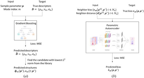
Figure 4. Prediction workflow of the two-machine framework.

3.3. Training database

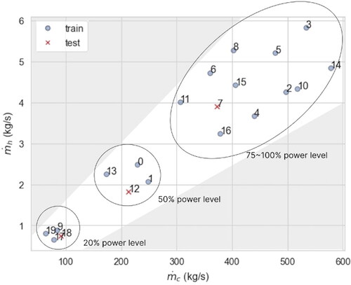
In this demonstration, the mass flows at the cold (main) and hot (branch) inlet, ${\dot{m}}_c$ and ${\dot{m}}_h,$ are selected as the input parameters. The design of experiment (DOE) is shown in Figure 5.

Figure 5. Design of experiment in terms of mass flux ratio, which corresponds to different power levels in a reactor operation.

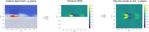
The time-history data is collected from the resampled plane at the recirculation region, as illustrated in Figure 6. A total of 576 equally spaced probes are resampled from the top of the recirculation region for snapshot collection. In each simulation, 4000 snapshots with time-step equal to 0.005 s are collected. Due to the presence of swirl-switching in the flow oscillations within the elbow-tee configuration, insufficient simulation time may lead to an incomplete capturing of the bi-stable state of the vortex movements. This can result in the observation of flow asymmetry in the y-direction and lead to asymmetries of POD modes. The presence of asymmetric POD modes can significantly affect the performance of the CNN-based structure corrector, as distinguishing between deformations caused by changes in boundary conditions and those resulting from flow asymmetry becomes challenging. One solution is to extend the simulation time, but this requires a significant computational workload for constructing a machine-learning database. To reduce simulation time, the POD in this research is performed on the $+y$ plane, and the resulting POD data is then mirrored onto the $-y$ plane to ensure data symmetry, as depicted in Figure 7. This approach helps to reduce the simulation time while maintaining the necessary data symmetry for correct analysis.

Figure 6. Illustration of data acquisition points. A total of 576 equally spaced probes are placed at the top region of the pipe to collect the flow snapshots from the high-fidelity simulations.

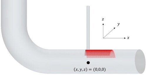
Figure 7. Schematics of the POD-mirroring. The data from the reduced data domain ($+y$ plane) is used to extract POD structures. The resulting spatial modes are mirrored to the $-y$ plane for imposing flow symmetry.

In this demonstration, 20 full-order CFD runs are performed for constructing the datasets. The 20 runs are split into two datasets: training (17 samples) and testing (3 samples). While this number may seem low, it is important to note that each simulation generates $4000\times 288$ data points, which is further decomposed into $r=20$ modes of spatial and temporal decompositions. Furthermore, the proposed two machine framework is designed to demonstrate its capability to work with the noted sample size, as large-scale applications will largely be constrained by the computational cost of the full-order simulations. In the proposed configuration, the cpu-time on single processor for a full-order simulation is ∼442 hr to obtain 10 sec quasi steady-state oscillations.

After conducting hyperparameter tuning, this work has employed 100 estimators for gradient boosting, with a maximum depth of 5 and a minimum number of samples required for a node to be split set to 3. The number of filters in the Parameterized CNN are 128 and 32 for the encoding and transport convolution, respectively.

4. Results

4.1. Flow snapshots visualization

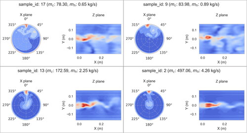
Figure 8 compares the flow snapshots of four selected samples with varying input mass flow rates, ranging from low to high. Here we show the instantaneous streamwise velocity on two planes (1)(1) $${\mathit{u}}_h\left(t;\mathit{\mu }\right)\approx {\widehat{\mathit{u}}}_h\left(t;\mathit{\mu }\right)=\sum _{m=0}^r{\mathit{\varphi }}_m{\mathrm{ }\left(\mathit{\mu }\right)a}_m\left(t;\mathit{\mu }\right)$$(1) the cross-sectional plane located 2$D_b$ downstream of the junction and (2)(2) $${\mathit{S}}^{\left(k\right)}=\left[{\mathit{u}}_{\mathit{h}}\left(t_1;{\mathit{\mu }}^{\left(k\right)}\right)\left|{\mathit{u}}_{\mathit{h}}\right(t_2;{\mathit{\mu }}^{\left(k\right)}\left)\right|\cdots \left|{\mathit{u}}_{\mathit{h}}\right(t_{N_t};{\mathit{\mu }}^{\left(k\right)})\right]$$(2) the full y-plane near the top surface of the junction. The results reveal that the flow regime and the size of the mixing region is significantly influenced by the boundary conditions. At low mass flow rates (as observed in sample 17 and sample 9), the mixing region is more widespread across the pipe, and no significant Dean vortices are observed in the flow. Consequently, a large region at the top of the pipe is impacted by the mixing. As the mass flow rate increases (as seen in sample 13 and sample 2), the formation of Dean vortices becomes more prominent. These vortices grow stronger and more concentrated toward the core of the pipe, resulting in a reduction in the size of mixing region near the wall.

Figure 8. Flow snapshots of streamwise velocity. For different mass flow rates, the results show high nonlinearity.

4.2. Coherent structures identification

In the present study, two main types of vortex shapes are observed in the given design space. The first type is characterized by large, elongated vortices, while the other type demonstrates vertical structures resembling the Karman vortex street, as depicted in Figure 9. The feasibility of using the reduced data domain for capturing POD modes is first examined to ensure that different types of vortices can be correctly identified. Figure 10 displays the POD structures extracted from the reduced $+y$ data window. Nearly identical vortical structures are observed, which suggests that employing the reduced domain is a viable strategy for imposing flow symmetry. In this study, the subsequent discussions will be based on the utilization of the $+y$ data window.

Figure 9. Two main types of vortical structures were obtained from performing POD on the full data window: (a) large, elongated vortices observed in low mass flow rate cases (sample 17) (b) von Karman vortex street type of vortices observed in high mass flow rate cases (sample 2).

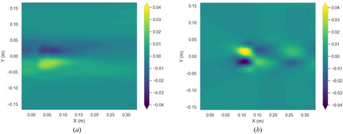
Figure 10. The first POD mode obtained from the reduced data window. (a) sample 17 (b) sample 2. The same vortical structures are obtained when comparing with Figure 9.

Within the operating range of the reactor, the oscillatory flow behavior exhibits significant variations. Figure 11 presents structure characteristics for 20% and 100% power levels. For 20% power level conditions (sample 17), the first two POD modes feature large, slow motions, while the third mode demonstrates the characteristics of vortex shedding. Conversely, at 100% power level (sample 2), vortex shedding becomes the predominant phenomenon for the first few modes. Small changes in input parameters within the same power level can also result in considerable differences in the dominating velocity structures, as illustrated in Figure 12(a). 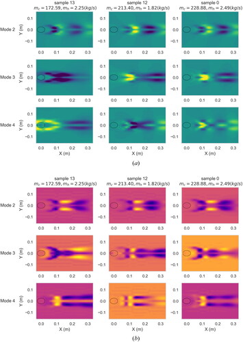Comparing sample 0 (${\dot{m}}_c$=228.88, ${\dot{m}}_h$=2.49 kg/s), sample 12 (${\dot{m}}_c$=219, ${\dot{m}}_h$=2.32 kg/s), and sample 13 (${\dot{m}}_c$=202.59, ${\dot{m}}_h$=2.02 kg/s), under operation condition of approximately 50% power level, reveals considerable differences in the spatial distribution of vortices. The POD modes of the temperature field are also presented in Figure 12(b). The structure shapes do not follow a monotonic trend either. This result implies that the impact of parametric change to turbulence mixing, and the consequent thermal striping is nonlinear. Variations in input parameters lead to phenomenological changes in flow separation near the bend, formation of Dean vortices and turbulence generation driven by shearing forces near the junction. Even though only two input parameters are considered, the nonlinearity of these phenomena poses a considerable challenge for traditional global data-driven reduced-order approaches [37–39]. This challenge is addressed in this work through a predict-and-correct approach, as presented in the next section.

Figure 11. The oscillatory characteristics of turbulence structures under different power levels but with the same mass flux ratio (∼40). (a) spatial modes. (b) Power spectrum density (PSD) for the temporal coefficients (unit: $m^2/s^2\mathit{\text{ Hz }}).$ In this example, sample 17 corresponds to the operating condition at 20% power level, whereas sample 2 represents the scenario at 100% power level.

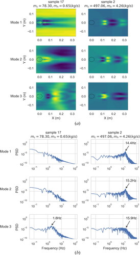
Figure 12. Flow structures deformation with slight parameter variations: (a) velocity field (b) temperature field. The presented samples depict flow conditions at approximately 50% power levels.

4.3. Structures prediction and correction

In the following sections, we present three testing samples (sample 7, 0, and 9) that are unseen by the machine learning framework. First, the structure predictor (referred to as machine 1) is tasked with determining the relationship between input parameters and structure characteristics, and selecting reference structures from the library based on the pre-processed descriptors. The performance of the structure predictor, M1, is shown in Figures 13 and 14. With the physic descriptors as output targets, the machine can choose the most resembling structures for the input parameters. The results show that the library look-up process is effective in selecting reference structures, which implies that the descriptors are informative in describing the vortex characteristics. Although the lookup results exhibit reasonable similarity, there exist differences in the spatial strength and the boundary locations, as expected. The second machine is used to address the bias.

Figure 13. Assessment of the structure predictor for velocity POD modes: (a) sample 7 (b) sample 0 (c) sample 9. The first row shows the temporal coefficients of the POD modes (in frequency domain). The second and third rows show the true and predicted structures, respectively.

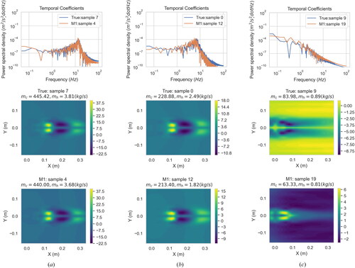
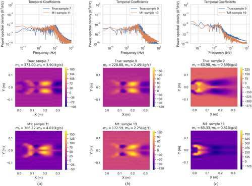
Figure 14. Assessment of the structure predictor for temperature POD modes: (a) sample 7 (b) sample 0 (c) sample 9. The first row shows the temporal coefficients of the POD modes (in frequency domain). The second and third rows show the true and predicted structures, respectively.

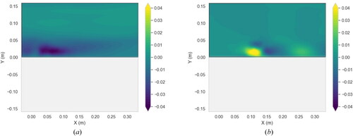
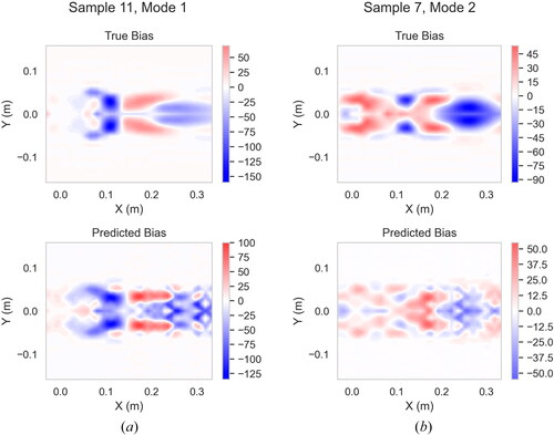
The biases predicted by the machine 2 (M2) are presented in Figure 15 (velocity) and Figure 16 (temperature). The term “true bias” refers to the bias that arises when using the reference structures to approximate the true structures, i.e. ${\mathit{ϵ}}_m\left(\mathit{\mu },{\mathit{\mu }}^{*}\right)={\mathit{\varphi }}_m({\mathit{\mu }}^{*}){-\mathit{\varphi }}_m(\mathit{\mu });$ the term “predicted bias” is the bias predicted by M2. The results show that, although there are local discrepancies between the true bias and predicted bias, the CNN-based M2 can generally identify the region where the structure deformation occurs due to parametric change.

Figure 15. Results of bias prediction: velocity (a) training: sample 11, mode 1 (b) Testing: sample 7, mode 1. The term true bias refers to the bias that arises when using the reference structures to approximate the true structures (i.e. ${\mathit{ϵ}}_m\left(\mathit{\mu },{\mathit{\mu }}^{*}\right)$); the predicted bias represents the M2 prediction (i.e. ${\widehat{\mathit{ϵ}}}_m\left(\mathit{\mu },{\mathit{\mu }}^{*}\right)$).

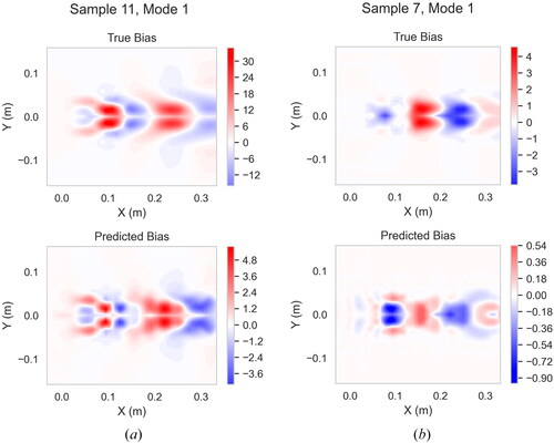
Figure 16. Results of bias prediction: temperature (a) training sample 11, mode 1 (b) testing: sample 7, mode 1. The term true bias refers to the bias that arises when using the reference structures to approximate the true structures (i.e. ${\mathit{ϵ}}_m\left(\mathit{\mu },{\mathit{\mu }}^{*}\right)$); the predicted bias represents the M2 prediction (i.e. ${\widehat{\mathit{ϵ}}}_m\left(\mathit{\mu },{\mathit{\mu }}^{*}\right)$).

4.4. Full prediction of velocity and temperature field

To demonstrate the efficacy of the proposed framework for thermal striping emulation, the standard deviation of the field fluctuations and the frequency responses are compared. Figure 17(a) and 17(b) show the $u_{\mathit{\text{rms}}}$ and $T_{\mathit{\text{rms}}}$ of three testing cases. As the M1 can successfully select the proper structures that exhibit similar oscillatory characteristics, the predicted standard deviations are very close to the true values, especially in the velocity field (Figure 17(a)). The results indicate that using reference structures to approximate the field is powerful in reconstructing the oscillatory signals. Compared to the velocity predictions, the approximation bias of M1 is higher in the temperature field, indicating that the temperature field is more sensitive to changes in boundary conditions. For such cases, in which the reference structures fail to provide good approximation bases (Figure 17(b)), the second machine (M2) can reduce the bias and achieve reasonable predictions. The root mean square errors (RMSE) of the three cases, over the total of 864 spatial locations, are 0.046 (m/s) and 1.180 (K) for $u_{\mathit{\text{rms}}}$ and $T_{\mathit{\text{rms}}}$ respectively. Figures 18 and 19 visualize the synthetic signals at the critical points where the $u_{\mathit{\text{rms}}}$ and $T_{\mathit{\text{rms}}}$ are peaked. The result shows that the framework prediction is consistent with the full-order model.

Figure 17. Field RMS prediction (a) $u_{\mathit{\text{rms}}}$ (b) $T_{\mathit{\text{rms}}}.$ The term “M1” refers to using structure predictor only; the term “M1 + M2” refers to using both structure predictor and structure corrector.

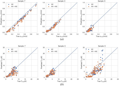
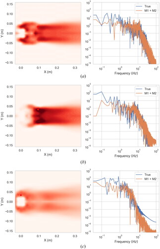
Figure 18. Emulation of velocity field. Signals with peak $u_{\mathit{\text{rms}}}$ magnitudes are presented. (a) sample 7 (b) sample 0 (c) sample 9 (Left: the probe location; the coloring indicates the $u_{\mathit{\text{rms}}}$ magnitude. Right: power spectrum density of the true/emulated velocity signals).

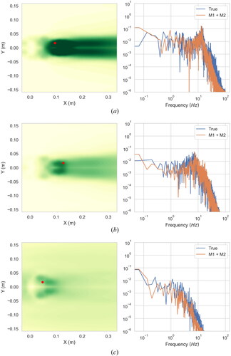
Figure 19. Emulation of temperature field. Signals with peak $T_{\mathit{\text{rms}}}$ magnitudes are presented. (a) sample 7 (b) sample 0 (c) sample 9 (Left: the probe location (Left: the probe location; the coloring indicates the $T_{\mathit{\text{rms}}}$ magnitude. Right: power spectrum density of the true/emulated velocity signals).

Table 2 compares the computational times for different stages of the process. The results show that the emulator significantly enhances the computational efficiency, achieving a speed-up factor of approximately ${10}^7.$ This highlights the potential of using emulators in accelerating the design and operation analysis for thermal striping assessment. Several key findings have been identified to enable the success of the data-driven approach. Firstly, a database of full-order solution samples is required to construct a library of coherent structures. The tradeoff between computational cost for generating sufficient samples and obtaining reasonable coverage of parametric variations should be appropriately considered. As the proposed framework utilizes the lookup-and-correct approach, it is important to note that the system’s accuracy will depend significantly on the quality of the structure library. The effectiveness of parameter extrapolation is limited to cases where similar structures are present within the structure library. Secondly, the presented framework is based on the identification of coherent turbulent structures, and may have limited applicability to phenomena that are not strongly impacted by large coherent structures, such as small-scale dissipation or wall effects. Additionally, we note that due to the computational burden of the full order runs, other deep learning algorithms, such as recurrent neural networks or long short-term memory networks, will require much larger training database. Moreover, their ability to interpolate to new data is questionable for parametric time-dependent problems. Thus, the proposed framework has chosen to rely on selecting appropriate coherent structures to emulate the oscillatory behaviors. Finally, although the practicality of using this approach for real application remains to be demonstrated, the framework has confirmed its capability to capture the fluctuations of spatiotemporal field, and has great potential to enable multi-query applications such as digital twin technologies and design evaluations. Furthermore, given the high similarity between the Karman vortex street and the vortices observed near the branch of the T-junction [16, 40, 41], the proposed framework has the great potential to extend its application to a broader scope of the flow pass bluff body problems, including airfoil design and wind field analysis around buildings, to mention a few.

Table 2. Computational times for the full-model CFD simulation (single processor) and the framework surrogate.

	Training time	Runtime
Full model	8,840 hr^1	442 hr (one full simulation)
Two-machine framework surrogate	Structure predictor: 11.8 ($s$) Structure corrector: 149$(\mathrm{\text{min}})$	0.78 ($s)$
Runtime Acceleration (Full-model / surrogate)-		7.57 E + 7

¹ Time for generating the training data (20 samples).

5. Conclusions

Mechanical and thermal fatigue failures remain key drivers for the operation and maintenance (O&M) activities for both operating and advanced nuclear reactors, and energy systems in general. For flow-assisted fatigue damage, high-resolution simulations are often necessary to capture the complex turbulence interactions. However, implementing a full-order simulation tool can be computationally overwhelming, particularly for industrial applications that require multi-query problem-solving, such as digital twin (DT) construction and design optimizations. Finding an efficient approach to model these interactions is crucial for effective and practical engineering solutions.

In this work, a two-level machine-learning framework for parametric thermal striping in industrial applications has been proposed and demonstrated. The framework is based on the resolution of turbulence coherent structure. The diagnostic view of local POD is adopted to construct a structure library for the designed parametric space; the down-selection and bias correction procedure are implemented. With the select-and-correct technique, the framework leverages the proximate library structures and avoids giving predictions that are excessively deviated from the design of experiments with a limited number of training samples.

A T-junction with a 90° upstream bend is selected as the target application, as it represents an often encountered configuration in reactor systems. With the two-level design, the framework can utilize the physical significance of the turbulence coherent structures and efficiently reduce the number of full-order simulations required for training. The results show that the framework can achieve prediction of the full-field distribution of spatial-temporal fluctuations. A speed-up factor of an order of ${10}^7$ has been obtained. In the fluid field, consistent agreement for both standard deviations and reconstructed temporal frequencies is observed. The RMSEs for 864 testing probes are respectively 0.046 (m/s) and 1.180 (K) for $u_{\mathit{\text{rms}}}$ and $T_{\mathit{\text{rms}}}.$ Our findings indicate that the emulated signals are highly consistent with the full-order model. The framework has demonstrated its capability to capture the fluctuations of spatiotemporal field. In practice, the proposed machine-learning emulator could serve as a fast-computing surrogate, replacing computationally intensive full-order model for thermal striping evaluation. This approach has great potential to enable multi-query applications such as digital twins technologies and design evaluations. In future work, an important direction lies in incorporating methods for uncertainty quantification and error estimation of the machine learning emulator.

Acknowledgements

The research is supported by the Generating Electricity Managed by Intelligent NuclearAccess (GEMINA) program of the U.S. Advanced Research Project Agency-Energy (ARPA-E) under Award Number [DE-AR0001295].