Network externalities, product compatibility and process innovation

ABSTRACT

This article augments d’Aspremont and Jacquemin’s [1988. “Cooperative and Noncooperative R&D in Duopoly with Spillovers.” American Economic Review 78: 1133–1137; 1990. “Cooperative and Noncooperative R&D in Duopoly with Spillovers: Erratum.” American Economic Review 80: 641–642] cost-reducing R&D duopoly by introducing network externalities and product compatibility and then considers the investment decision stage. For standard non-network industries, the received literature has robustly shown that the non-cooperative R&D investment decision game is, without technological spill-over, a prisoner’s dilemma with investing firms (there is a conflict between self-interest and mutual benefit of investing in R&D), and a deadlock (there is no conflict between self-interest and mutual benefit of investing in R&D) only whether the extent of technological spill-over is sufficiently high. Network externalities and product compatibility challenge this result. In fact, outcomes antithetical to those emerging in a non-network industry do exist. Under symmetric full compatibility, the game is a deadlock also without spill-over effects. Under symmetric incompatibility, the game can be a prisoner’s dilemma irrespective of the extent of the technological spill-over. From a policy perspective, the article shows that R&D subsidies or taxes can be used as social welfare maximising tools depending on the extent of the network externality and the degree of product compatibility. The work focuses on Cournot rivalry, but results hold also for price-setting firms (Bertrand rivalry).

KEYWORDS:

• Process innovation
• Nash equilibrium
• network externality
• product compatibility
• R&D subsidies and taxes

JEL CLASSIFICATION:

• D43
• L13
• O31

1. Introduction

This research aims at contributing to two strands of the industrial organisation (IO) literature: (1) the literature on cost-reducing R&D investments (process innovation), following the d’Aspremont and Jacquemin’s (1988, 1990) seminal contributions (AJ henceforth), and (2) the literature on markets with network externalities and product compatibility, along the line of Katz and Shapiro (1985). As known, network industries – e.g. telecommunications and software – are rapidly developing in modern economies, and they are generally characterised by an oligopolistic structure.

The first strand of the literature focuses on oligopoly markets in which firms invest in process innovation R&D (see, e.g. Henriques 1990; De Bondt, Slaets, and Cassiman 1992; Kamien, Muller, and Zang 1992; Suzumura 1992; Kamien and Zang 2000; Atallah 2004; Chen and Nie 2014; Marini, Petit, and Sestini 2014; Nie and Wang 2019).¹ In these contributions, the authors concentrate on models with strategic interactions in which firms are generally engaged in a two-stage sequential game: at the first stage, they choose the extent of cost-reducing R&D investments, in turn affecting the competitive position of each firm operating in the product market; at the second stage, they compete in the product market (by generally considering the case of Cournot rivalry). Bacchiega, Lambertini, and Mantovani (2010) and Buccella, Fanti, and Gori (2021a) offer a different perspective on this issue. Both add a stage to the two-stage AJ’s game: a first stage in which firms non-cooperatively decide whether to invest in cost-reducing R&D. The former finds that this three-stage R&D game is always a prisoner’s dilemma (there is a conflict between self-interest and mutual benefit of investing in R&D), unless a parameter region with sufficiently large values of R&D spillovers in which the prisoner’s dilemma is solved and the game turns to be an anti-prisoner’s dilemma or deadlock (there is no conflict between self-interest and mutual benefit of investing in R&D). The latter generalises on the former model to horizontal product differentiation and shows that differentiation can eliminate the prisoner’s dilemma also in the absence of spill-over effects. This result is interesting for, at least, a twofold reason: (i) the prisoner’s dilemma is an unpleasant outcome for firms and, therefore, R&D investment results to be Pareto-inferior from a societal perspective; (ii) as Buccella, Fanti, and Gori (2021b) show, the robust outcome according to a correct game-theoretic approach, in which firms choose whether to disclose information about R&D investments, is the absence of R&D spillovers. The existence of a prisoner’s dilemma means that R&D competition will tend to ruin firms and explains the incentive to form an R&D cartel, as an alternative to non-cooperative R&D.

In this regard, Burr, Knauff, and Stepanova (2013) provide an interesting explanation of the prisoner’s dilemma emerging in the AJ setting. They concentrate on the role of the spill-over parameter and the extent of the efficiency of the R&D technology play: on one hand, due to the well-known free riding effect of the public goods, high spillovers are always expected to reduce firms’ incentives towards R&D, and thus also tend to reduce the prisoner’s dilemma loss of profitability. Additionally, higher costs of R&D always reduce the engagement in R&D, and thus indirectly reduce the prisoner’s dilemma loss of profitability. On the other hand, when firms engage in non-cooperative R&D and are entrapped in a profit-worsening dilemma, consumers are better off; moreover, these benefits more than offset the negative impact on firms’ profits, and thus social welfare increases. However, the increase in social welfare following the firms’ decision to invest in R&D cannot represent a Pareto-superior outcome as consumers are better off but firms are worse off compared to a scenario in which firms do not invest in R&D. The mechanism detailed by Buccella, Fanti, and Gori (2021a) solves the dilemma through horizontal product differentiation. This article shows another – more elaborate – mechanism (network externalities and product compatibility) that aims at solving the dilemma emerging in the AJ setting.

Regarding the second strand, a pioneering work dealing with process innovations in markets with network goods is Boivin and Vencatachellum (2002), in which the authors pinpoint the role of network effects in increasing the extent of R&D investments. More recently, Naskar and Pal (2020) compare non-cooperative R&D investments in process innovation under different competition modes (Cournot and Bertrand settings) in the product market, and Shrivastav (2021) generalises on the previous work by assuming a wider range of network compatibility, allowing to move from no compatibility to full compatibility. Other two works dealing with similar issues in the AJ setting are Knauff and Karbowski (2021), who analyse non-cooperative and cooperative R&D in markets with network effects and incomplete product compatibility, and Heywood, Wang, and Ye (2022), who compare R&D competition and R&D cooperation in an incumbent-entrant economy à la AJ with endogenous network compatibility. The former study shows that the network externality may reverse the common wisdom that cooperative behaviour in innovation is better off from a societal perspective; consequently, policy interventions promoting R&D cooperation between firms can be counterproductive. The latter one identifies conditions for which complete incompatibility (a) occurs more likely under cooperative R&D than under non-cooperative R&D, and (b) generates a large gap in R&D effort and profits between incumbent and entrant.

None of these works, however, concentrates on the endogenous emergence of Nash equilibria by comparing the strategic incentive of quantity-setting or price-setting firms whether to invest in R&D by taking the AJ setting with and without spillovers as a basic framework. This article departs from Naskar and Pal (2020) and Shrivastav (2021) and aims to re-considering the AJ non-cooperative game at both the R&D stage and market stage by adding the investment decisions stage to the two-stage set up along the lines of Bacchiega, Lambertini, and Mantovani (2010) and Buccella, Fanti, and Gori (2021a). For doing this, it augments the AJ setting with (positive and negative) network externalities and product compatibility. Specifically, Bacchiega, Lambertini, and Mantovani (2010) were the first to introduce the investment decision stage to the two-stage AJ Cournot game with process innovation by assuming homogeneous products. They showed the existence of: (1) a parameter region, identified by the interplay between the extent of technological spillovers and the efficiency of the R&D activity, in which the three-stage non-cooperative R&D game is a prisoner’s dilemma (low values of R&D spillovers or no spillovers), so that investing in R&D results in profit reduction; (2) a parameter region in which the prisoner’s dilemma is solved and the game turns to be an anti-prisoner’s dilemma (larger values of R&D spillovers), so that investing in R&D results in profit gain. By assuming heterogeneous products (horizontal products differentiation), Buccella, Fanti, and Gori (2021a) re-considered the investment decision game showing that product differentiation can solve the dilemma also in the absence of spill-over effects, so that investing in R&D results in profit gains irrespective of the main parameters of the problem. They also showed that R&D subsidies can be used as a welfare-maximising tool with or without R&D spillovers extending Amir et al. (2019).

The present work follows this path (endogenous game) by assuming a network industry with product (in)compatibility, showing that a twofold novel outcome emerges: (i) under symmetric full compatibility, in the absence of both R&D spillovers and product differentiation, a sufficiently intense network effect eliminates the prisoner’s dilemma; (ii) under symmetric no compatibility, the game is a prisoner’s dilemma also in the case of full disclosure.² Both results are exclusive to network industries and are antithetical to those emerging in the standard non-network setting (Bacchiega, Lambertini, and Mantovani 2010; Buccella, Fanti, and Gori 2021a), in which (a) with no disclosure and without product differentiation, the Nash equilibrium is a prisoner’s dilemma with investing firms, and (b) with high or full disclosure, the Nash equilibrium is an anti-prisoner’s dilemma with investing firms regardless of whether products are homogeneous or heterogeneous.

From a policy perspective, in markets with positive network externalities, policymakers aiming to reach a Pareto-superior outcome may abstain to intervene directly in the case of full compatibility and incentivise a higher degree of compatibility in the case of low compatibility. However, as designing an ad hoc public incentive towards product compatibility may be difficult to implement – as it represents a marketing strategy related to customers’ preferences requiring identifying several product characteristics and information that may be very costly for the public authority –, the present article shows that: (1) R&D subsidies can be used as a welfare-maximising tool regardless of whether network externalities are positive or negative in the case of symmetric full compatibility; (2) R&D subsidies or taxes can be used as a welfare-maximising tool depending on the size of the network externalities in the case of symmetric partial compatibility or no compatibility. If the network externality is negative (or it is positive, but its strength is sufficiently low), it is optimal to subsidise R&D to favour the effort towards process innovation investments. This is because the amount of R&D emerging from firms’ decisions in the market is too low (and the output accordingly) compared to the social optimum. If the network externality is positive and its strength is sufficiently high, it is optimal to tax R&D to disincentive the effort towards process innovation investments. This is because the amount of R&D emerging from firms’ decisions in the market is too high (and the output accordingly) compared to the social optimum.

This work is part of a growing IO literature stressing the importance of networking in strategic contexts (e.g. Choi, Kim, and Lee 2010; Hoernig 2012; Bond-Smith 2019; Dan 2019; Fanti and Gori 2019), and aims also at providing a basic model for econometricians to test whether in network industries there should be more R&D effort and larger profits than in the absence of networks.

The article definitively extends the literature in two directions. From a game-theoretic point of view, it adds the investment decision stage to the two-stage AJ setting with (positive and negative) network externalities and product compatibility. In this regard, it departs from Naskar and Pal (2020) and Shrivastav (2021) and follows the route detailed by Bacchiega, Lambertini, and Mantovani (2010) and Buccella, Fanti, and Gori (2021a), showing a novel mechanism through which the Nash equilibrium outcomes can change compared to the basic R&D framework (non-network and homogeneous products). From a policy perspective, it follows Amir et al. (2019) and shows the role that R&D subsidies can have in a network industry stressing similarities and differences of using this instrument to incentivise private R&D effort compared to the standard non-network setting. However, unlike Amir et al. (2019) and the related literature on this issue, it pinpoints the role of R&D taxes as a welfare-maximising tool. This indeed opens the route to the use of a disincentive fiscal devise to the R&D activity to avoid over-investment depending on the relative weight of the network strength and the degree of product compatibility.

The remainder of the article is organised as follows. Section 2 outlines the model with quantity-setting firms and discusses the main ingredients of the R&D investment decision game augmented with positive and negative network externalities and product compatibility. Section 3 (resp. 4) studies the R&D investment decision game with network effects and symmetric full compatibility (incompatibility). Section 5 compares the equilibrium outcomes between full compatibility and incompatibility. Section 6 introduces the R&D subsidy (or tax) as a welfare maximising tool in an environment with network externalities. Section 7 extends the work by considering the degree of compatibility as an endogenous variable and discusses the compatibility decision game. Section 8 concludes the article. The Appendix provides analytical details and the proofs of the propositions. The online Appendix presents the model with the more general scenario of symmetric imperfect compatibility and the analysis at the different stages of the game, including the cases presented in the main text.

2. The model

Consider an economy with two types of agents: firms and consumers. On the supply side, the economy is bi-sectorial with a competitive sector producing the numeraire good $m$ and a duopolistic sector in which firm $i$ and firm $j$ ($i=\{1,2\}i\ne j$) produce goods of variety $i$ and variety $j$, respectively. These goods are perceived as homogeneous by customers. Firms also face the perspective of investing in cost-reducing R&D (process innovation) along the line of AJ. On the demand side, there exists a continuum of identical consumers with preferences described by a separable utility function $V(q_i,q_j,y_i,y_j,m)$, which is linear in the numeraire good $m$. The representative consumer maximises $V(q_i,q_j,y_i,y_j,m)=U(q_i,q_j,y_i,y_j)+m$ subject to the budget constraint $p_i{q}_i+p_j{q}_j+m=R$, where $U$ is a twice continuously differentiable function, $q_i$ and $q_j$ are the control variables of the problem, $p_i$ and $p_j$ represent the price of (i.e. the marginal willingness to pay of the representative consumer for) product of variety $i$ and variety $j$, respectively, and $R$ is the consumer’s exogenous nominal income. This income is assumed to be high enough to avoid income effects on the demand of $q_i$ and $q_j$ (i.e. the goods entering non-linearly in $V$). In this regard, in fact, the utility function $V$ is quasi-linear in $m$ so that all the related properties about the demand of $m$ and that of $q_i$ and $q_j$ hold (Amir, Erickson, and Jin 2017; Choné and Linnemer 2020).

Different from the traditional IO literature, we assume the existence of network externalities in consumption, i.e. one person’s demand also depends on the demand of other customers. In this regard, $y_i$ represents an external effect denoting the consumers’ expectations about firm $i$’s equilibrium total sales.

The simple mechanism of network effects described so far follows the seminal work of Katz and Shapiro (1985), used in several recent articles³ belonging to the IO literature framed in strategic competitive markets with (Naskar and Pal 2020; Shrivastav 2021) and without (Hoernig 2012; Chirco and Scrimitore 2013; Bhattacharjee and Pal 2014; Song and Wang 2017; Pal 2014, 2015; Fanti and Gori 2019) process innovation.

The function $U$ follows the usual specification of a quadratic utility: (1) $U=q_i+q_j-\frac{1}{2}(q_i^2+q_j^2+2q_i{q}_j)+n[q_i(y_i+k_i{y}_j)+q_j(y_j+k_j{y}_i)]-\frac{n}{2}(y_i^2+y_j^2+2k_i{y}_j{k}_j{y}_i)$(1) where $-1\le n\le 1$ is the strength of the network effect ($n=0$ represents the standard case of non-network goods). Positive (resp. negative) values of $n$ reflect a positive (resp. negative) consumption externality. Though several network industries exhibit positive externalities (mobile communications, software, internet-related activities, online social networks, fashion, etc.), as a greater number of users contribute to increase the value of the product to each consumer (there exists a positive feedback loop if the network becomes more valuable), one may think about real-world industries that exhibit both kinds of externalities. In this regard, the automobile industry is worth to be mentioned. This industry might also show negative consumption externalities as the more cars are sold, the greater the traffic congestion, parking difficulties and other related issues are. Therefore, a negative network externality implies that an increasing number of users reduces the value of the goods for each consumer (for instance, traffic congestion or network congestion over limited bandwidth). The terms $y_i+k_i{y}_j$ and $y_j+k_j{y}_i$ represent the expected effective network size of firm $i$’s consumers and of firm $j$’s consumers, respectively. The parameter $0\le k_i\le 1$ measures the degree of compatibility of the network of product $j$ towards the network of product $i$. Pairwise, the parameter $0\le k_j\le 1$ measures the degree of compatibility of the network of product $i$ with the network of product $j$. For example, $k_i=1$ implies that the network of product $j$ is perfectly compatible with the network of product $i$ (full compatibility), whereas $k_i=0$ implies that the network of product $j$ is perfectly incompatible with the network of product $i$ (no compatibility). The intermediate cases $0<k_i<1$ represent different degrees of imperfect or asymmetric compatibility of the network of product $j$ with the network of product $i$. For analytical tractability, the article will concentrate on the following two symmetric cases (without compromising generality) to study the emergence of Nash equilibria of the R&D investment decision game with network externality and product compatibility.

• First, $k_i=k_j=1$, implying symmetric full compatibility between the two networks.

• Second, $k_i=k_j=0$, implying symmetric incompatibility between the two networks.

The more general case of symmetric imperfect compatibility ($k_i=k_j=k$) and the analytical derivations of the reaction functions at the different stages of the game, from which one can also disentangle the two main polar scenarios discussed in the article, are presented in the online Appendix.

The asymmetric case $k_i\ne k_j$ – implying asymmetric compatibility of the network of product $j$ towards the network of product $i$ (including the cases of asymmetric extreme (in)compatibility implying full compatibility of one of the two networks and no compatibility of the other one, i.e. $k_i=1$ and $k_j=0$ or $k_i=0$ and $k_j=1$) – is not presented to save space, but nothing changes compared to the symmetric cases that will be studied later in the article.

The solution of the constrained utility maximisation gives the following linear inverse demand for product of variety $i$: (2) $p_i=1-q_i-q_j+n(y_i+k_i{y}_j),i,j=\{1,2\},i\ne j.$(2) As is clear from the expression in (2), the network externality enters additively in the market demand for product $i$. If the network externality is positive (resp. negative), an increase in the feedback loop of the network causes an outward (resp. inward) shift in the demand curve that, in turn, implies an increase (resp. reduction) in the quantity bought by consumers for any given value of the price. This externality therefore acts as a device that increases (resp. reduces) the market size. Though $q_i$ and $q_j$ are homogeneous goods, the marginal willingness to pay of consumers for product $i$ and product $j$ is generally different because of the different degree of compatibility between the two networks or, alternatively, because of the different effort exerted in the market of product $i$ and the market of product $j$ by the degree of compatibility in the cases of symmetric imperfect compatibility ($k_i=k_j=k$) and symmetric no compatibility ($k_i=k_j=0$). In the former case, in fact, the marginal willingness to pay for product $i$ and product $j$ is respectively given by $p_i=1-q_i-q_j+n(y_i+k{y}_j)$ and $p_j=1-q_j-q_i+n(y_j+k{y}_i)$. In the latter case, we have that $p_i=1-q_i-q_j+n{y}_i$ and $p_j=1-q_j-q_i+n{y}_j$. Only in the case of symmetric perfect or full compatibility ($k_i=k_j=1$), the marginal willingness to pay for product of network $i$ and for product of network $j$ is the same, i.e. $p_i=p_j=1-q_i-q_j+n(y_i+y_j)$. As we will see later in this article, however, by assuming that consumers have rational expectations (i.e. $q_i=y_i$ and $q_j=y_j$ hold in equilibrium), we will have that the equality $q_i^{\ast }=q_j^{\ast }$ holds as the equilibrium outcome of each symmetric sub-game. Therefore, under the assumption of symmetric compatibility ($k_i=k_j=k$), including the polar cases of full compatibility ($k_i=k_j=1$) and no compatibility ($k_i=k_j=0$) between the two networks, the marginal willingness to pay of consumers at the equilibrium will be the same for both products and given by $p_i^{\ast }=p_j^{\ast }=1-[2-n(1+k)]q_i^{\ast }\ge 0$.

Under symmetric full compatibility, the externality generated by the expected effective network size is the highest in both cases of positive and negative network effects, so that the external effect due to the consumers’ expectations about firm $j$’s equilibrium total sales affects the demand of product of network $i$ at the highest degree, strengthening the external effect due to the consumers’ expectations about firm $i$’s equilibrium total sales at its maximum intensity. Under symmetric incompatibility, this strengthening effect does not exist, and the externality generated by the expected effective network size is the lowest in both cases of positive and negative network effects. In this case, the demand of network $i$ is positively or negatively affected only by the external effect generated by the consumers’ expectations about firm $i$’s equilibrium total sales.

The total cost of production and the cost of R&D effort of firm $i$ are respectively given by the functions $C_i(q_i,x_i,x_j)$ and $X_i(x_i)$, where $x_i$ and $x_j$ represent the R&D effort (investment) firm $i$ and firm $j$ exert, respectively. Following AJ, these functions can be specialised by using the expressions: (3) $C_i(q_i,x_i,x_j)=(w-x_i-\beta x_j)q_i,i,j=\{1,2\},i\ne j,$(3) and (4) $X_i(x_i)=\frac{g}{2}{x}_i^2,i=\{1,2\},i\ne j,$(4) where $g>0$ is a parameter measuring R&D efficiency scaling up/down R&D investment total costs. It represents an exogenous index of technological progress measuring, for example, the appearance of a new, cost-effective technology, weighting the degree at which the available technology for process innovation affects investment decisions and firm’s profits. A reduction in $g$ can be interpreted as a technological advance so that investing in R&D becomes cheaper (i.e. the efficiency of R&D investment increases). In addition, $\beta \in [0,1]$ captures the extent of technological spillovers (externality) resulting from the R&D investment activity of firm $j$ exogenously flowing as a cost-reducing device towards firm $i$ (i.e. the amount of information that firm $j$ exogenously discloses). We assume that both firms symmetrically share this characteristic of the extent of technological spillovers. This scenario represents the standard case of exogenous spillovers – with respect to which a fixed fraction of a firm’s R&D process innovation exogenously flows to competitors, so that each firm has no direct control over the extent of disclosure for, e.g. technological reasons – and directly follows AJ and the subsequent contributions by Henriques (1990), Suzumura (1992), Kamien, Muller, and Zang (1992), De Bondt (1996), Bacchiega, Lambertini, and Mantovani (2010) and Buccella, Fanti, and Gori (2021a). When $\beta =0$, there are no R&D externalities, resembling the case of non-disclosure of R&D information. When $\beta =1$, R&D information is fully shared, so that R&D disclosure is at its (exogenous) highest intensity. As was discussed in the introduction, assuming $\beta >0$ is reasonable; however, this case cannot emerge as a SPNE of the non-cooperative disclosure decision game in the absence of R&D subsidies (see Buccella, Fanti, and Gori 2021b for details) in a standard non-network duopoly with Cournot investing firms, whereas it can emerge as a Nash equilibrium strategy if there are network externalities.

The expression representing the firm’s technology in Equation (3) implies that the unitary cost of production should be positive so that $w-x_i-\beta x_j>0$ must hold, where $0<w<1$ measures the unitary technology of production cost irrespective of R&D investments. Moreover, the expression representing the cost of R&D effort in Equation (4) reveals diminishing returns in the R&D technology exerted by firm $i$. Therefore, each firm sustains the cost of R&D effort with a technology displaying decreasing returns to scale to achieve the benefit of reducing the total unit costs of production with constant returns to scale.

Definitively, selfish firms are engaged in a three-stage non-cooperative R&D investment decision game with network externality, compatibility and complete information in which each of them chooses whether to invest in R&D activities at stage one (the investment-decision stage). At stage two (the R&D stage), firms choose the extent of their own process innovation R&D investments or, alternatively, they do not invest in R&D. At stage three (the market stage), firms compete on quantity in the product market. As is usual from Katz and Shapiro (1985), Hoernig (2012) Naskar and Pal (2020) and Shrivastav (2021), we assume that consumers have rational expectations. Therefore, at the third stage of the game we assume that $q_i=y_i$ and $q_j=y_j$ hold in equilibrium. The game is solved by adopting the backward induction logic.

Before proceeding further, we briefly sketch the firm’s profit maximisation programme considering the subgames in which both firms do (not) invest in R&D and when only one of them invests in R&D.

By using Equations (2), (3), and (4), the profit function of firm $i$ when they both symmetrically choose to invest in R&D, that is $x_i>0$ and $X_i(x_i)>0$ ($i=\{1,2\},i\ne j$) can be written as follows (5) ${\mathrm{\Pi }}_i^{I/I}=[1-q_i-q_j+n(y_i+k_i{y}_j)-w+x_i+\beta x_j]q_i-\frac{g}{2}{x}_i^2,i,j=\{1,2\},i\ne j,$(5) where the upper script I/I stands for universal positive R&D investments. Differently, if they both choose to do not invest in R&D, that is $x_i=0$ and $X_i(x_i)=0$ ($i=\{1,2\},i\ne j$), Equation (5) boils down to: (6) ${\mathrm{\Pi }}_i^{NI/NI}=[1-q_i-q_j+n(y_i+k_i{y}_j)-w]q_i,$(6) where the upper script NI/NI stands for universal no R&D investments.

Finally, if the R&D investment of firm $i$ is positive and the R&D investment of firm $j$ is zero, we have that $x_i>0$ and $X_i(x_i)>0$, and $x_j=0$ and $X_j(x_j)=0$. On the one hand, firm $i$ invests in process innovation, thus reducing its own average and marginal production costs but does not benefit from any stream of knowledge (externality) related to firm $j$’s R&D activity, which is absent in this case. On the other hand, firm $j$ does not invest in process innovation, but it can benefit from a stream of knowledge (externality) related to firm $i$’s R&D activity, whose extent is measured by the parameter $\beta$. Therefore, the profit functions of firms $i$ and $j$ now read respectively as follows: (7) ${\mathrm{\Pi }}_i^{I/NI}=[1-q_i-q_j+n(y_i+k_i{y}_j)-w+x_i]q_i-\frac{g}{2}{x}_i^2,$(7) and (8) ${\mathrm{\Pi }}_j^{I/NI}=[1-q_j-q_i+n(y_j+k_j{y}_i)-w+\beta x_i]q_j,$(8) where the upper script I/NI stands for positive R&D investments of firm $i$ and no R&D investments of firm $j$.

The next sections will concentrate on the analysis of the equilibrium values of the symmetric subgames in the which both firms do (not) invest in R&D and the asymmetric subgames in which only one of them chooses to sustain the cost of the R&D effort. This will be done by considering the cases detailed above, i.e. $k_i=k_j=1$ (symmetric full compatibility), $k_i=k_j=0$ (symmetric full incompatibility). We skip the general case $k_i\ne k_j$ to avoid unnecessary analytical complications. In doing so, the sections will also highlight and disentangle the role played by the stability conditions and the R&D cost conditions in defining the feasible parametric space identified by the extent of technological spillovers, and the efficiency of the R&D technology for the emergence of Nash equilibria in the R&D investment decision game with network effects and product compatibility.⁴

3. The R&D investment decision game with network effects and symmetric full compatibility

Let us assume that $k_i=k_j=1$. Profit maximisation at the different stages of the game allows us to compute the equilibrium values of output, R&D investments and profits in the symmetric subgames I/I and NI/NI as well as in the asymmetric subgame I/NI, which we summarise as follows along with the relevant thresholds that should be fulfilled for feasibility purposes to identify correctly the Nash equilibria of the game, that is, the stability conditions (distinguishing between strategic substitutability and strategic complementary of the R&D investments of both firms) and the R&D cost conditions (implying that the unitary cost of production should be positive in both the symmetric and asymmetric subgames).

The main equilibrium equations of the model with symmetric full compatibility are therefore the following: (9) $x_i^{\ast I/I}(1,1)=\frac{2(1-w)[1+(1-\beta )(1-n)]}{g{(3-2n)}^2-2(1+\beta )[1+(1-\beta )(1-n)]},$(9) (10) $q_i^{\ast I/I}(1,1)=\frac{g(1-w)(3-2n)}{g{(3-2n)}^2-2(1+\beta )[1+(1-\beta )(1-n)]},$(10) (11) ${\mathrm{\Pi }}_i^{\ast I/I}(1,1)=\frac{g{(1-w)}^2\{g{(3-2n)}^2-2{[1+(1-\beta )(1-n)]}^2\}}{{\{g{(3-2n)}^2-2(1+\beta )[1+(1-\beta )(1-n)]\}}^2},$(11) where $g>\frac{2(1+\beta )[1+(1-\beta )(1-n)]}{{(3-2n)}^2}:=g_{SC}^{{\beta }_{high}}(\beta ,n)$, which will be clarified later (see Equation (21)), must hold to guarantee positive values of R&D effort and production in the subgame I/I, and $g>\frac{2{[1+(1-\beta )(1-n)]}^2}{{(3-2n)}^2}:=g_{SOC}(\beta ,n)$ must hold to guarantee correspondingly positive profits. The subscripts $SC$ and $SOC$ denote ‘Stability Condition’ and ‘Second Order Condition’, respectively. These inequalities will be clarified later. The term $(1,1)$ stands for symmetric full compatibility ($k_i=k_j=1$). In addition, we have that: (12) $q_i^{\ast NI/NI}(1,1)=\frac{1-w}{3-2n},$(12) (13) ${\mathrm{\Pi }}_i^{\ast NI/NI}(1,1)=\frac{{(1-w)}^2}{{(3-2n)}^2},$(13) and (14) $x_i^{\ast I/NI}(1,1)=\frac{2(1-w)[1+(1-\beta )(1-n)]}{g{(3-2n)}^2-2{[1+(1-\beta )(1-n)]}^2},$(14) (15) $q_i^{\ast I/NI}(1,1)=\frac{g(1-w)(3-2n)}{g{(3-2n)}^2-2{[1+(1-\beta )(1-n)]}^2},$(15) (16) $q_j^{\ast I/NI}(1,1)=\frac{(1-w)\{g(3-2n)-2(1-\beta )[1+(1-\beta )(1-n)]\}}{g{(3-2n)}^2-2{[1+(1-\beta )(1-n)]}^2},$(16) (17) ${\mathrm{\Pi }}_i^{\ast I/NI}(1,1)=\frac{g{(1-w)}^2}{g{(3-2n)}^2-2{[1+(1-\beta )(1-n)]}^2},$(17) (18) ${\mathrm{\Pi }}_j^{\ast I/NI}(1,1)=\frac{{(1-w)}^2{\{g(3-2n)-2(1-\beta )[1+(1-\beta )(1-n)]\}}^2}{{\{g{(3-2n)}^2-2{[1+(1-\beta )(1-n)]}^2\}}^2},$(18) where $g>g_{SOC}(\beta ,n)$ must hold to guarantee positive values of R&D effort, production and profits of the investing firm $i$, and $g>\frac{2(1-\beta )[1+(1-\beta )(1-n)]}{3-2n}:=g_{SC}^{{\beta }_{low}}(\beta ,n)$, which will be clarified later (see Equation (20)), must hold to guarantee positive values of production of the non-investing firm $j$.

The second-order condition for a maximum (concavity) requires that ${\frac{{\mathrm{\partial }}^2{\mathrm{\Pi }}_i^{I/I}(x_i,x_j)}{\mathrm{\partial }{x}_i^2}|}_{x_i=x_i^{\ast I/I}}<0$. This implies that the inequality (19) $g>\frac{2{[1+(1-\beta )(1-n)]}^2}{{(3-2n)}^2}:=g_{SOC}(\beta ,n)(\mathrm{second}\text{-}\mathrm{order}\mathrm{condition}),$(19) must hold to guarantee that the solution to the profit maximisation problem is economically meaningful. This condition boils down to $g>g_{SOC}(\beta ,0):=\frac{2}{9}(2-\beta {)}^2$ if $n=0$ (non-network economy), which replicates exactly the AJ’s result in our normalised setup. The R&D equilibrium characterised by the expression in (9) is stable (in the sense of Seade 1980) if and only if the reaction functions defined in the R&D space adequately cross (Henriques 1990). Indeed, Henriques (1990), Bacchiega, Lambertini, and Mantovani (2010), Hinloopen (2015), Buccella, Fanti, and Gori (2021a) find that the R&D reaction curves can be downward or upward sloping depending on the relative size of $\beta$ (the R&D externality). If those are downward sloping (resp. upward sloping), $x_i$ and $x_j$ are strategic substitutes (resp. complements). This holds when the R&D externality is small (resp. large). The stability conditions require that $\left|\frac{d{x}_i}{d{x}_j}\right|<1$ in both cases of strategic substitutability and complementarity, leading to a relationship only between $g$ and $\beta$ if $n=0$. Differently, the R&D reaction curves in the case of network externalities and symmetric full compatibility can be downward sloping or upward sloping depending on the relative size of $\beta$ and $n$. Consequently, the stability conditions include three parameters ($g$, $\beta$ and $n$). In this regard, one should compute $\frac{d{x}_i}{d{x}_j}$ and evaluate its sign. Therefore, $\frac{d{x}_i}{d{x}_j}<0$ if and only if $\beta <\frac{1-n}{2-n}$ ($x_i$ and $x_j$ are strategic substitutes) and $\frac{d{x}_i}{d{x}_j}>0$ if and only if $\beta >\frac{1-n}{2-n}$ ($x_i$ and $x_j$ are strategic complements). Definitively, the stability conditions $\left|\frac{d{x}_i}{d{x}_j}\right|<1$ in the R&D model with network externalities and symmetric full compatibility are the following: (20) $g>g_{SC}^{{\beta }_{low}}(\beta ,n)=\frac{2(1-\beta )[1+(1-\beta )(1-n)]}{3-2n}\mathrm{if}0\le \beta <\frac{1-n}{2-n},(x_{i}and{x}_i\mathrm{are}\mathrm{strategic}\mathrm{substitutes}),$(20) and (21) $g>g_{SC}^{{\beta }_{high}}(\beta ,n)=\frac{2(1+\beta )[1+(1-\beta )(1-n)]}{{(3-2n)}^2}\mathrm{if}\frac{1-n}{2-n}<\beta \le 1,(x_i\mathrm{and}{x}_j\mathrm{are}\mathrm{strategic}\mathrm{complements}),$(21) where $g_{SC}^{{\beta }_{low}}(\beta ,n)>g_{SC}^{{\beta }_{high}}(\beta ,n)$ for any $0\le \beta \le \frac{1-n}{2-n}$ and $g_{SC}^{{\beta }_{low}}(\beta ,n)<g_{SC}^{{\beta }_{high}}(\beta ,n)$ for any $\frac{1-n}{2-n}\le \beta \le 1$. Therefore, the condition that guarantees positive R&D investments ($g>g_{SC}^{{\beta }_{high}}(\beta ,n)$) from Equation (9) and the second-order condition ($g>g_{SOC}(\beta ,n)$) are fulfilled for any $0\le \beta \le 1$ if the stability conditions are satisfied. In other words, the second-order condition is always verified if the stability conditions are fulfilled. We basically recall that the second-order condition and the stability conditions suggest that the efficiency of R&D activity should not be too high, i.e. parameter $g$ should not be too low to avoid excessive R&D investments that would contribute to reduce greatly marginal and average production costs and increase output, pushing down the market price of products of both networks. Combining these results with Equations (9)–(11) allows us to state the following propositions.

Proposition 3.1:

[Positive externality, $0<n\le 1$]. An increase in the strength of the positive network effect ($n\uparrow$) under symmetric full compatibility ($k_i=k_j=1$) increases R&D effort, production and profits in the subgame I/I. [Negative externality, $-1\le n<0$]. An increase in the strength of the negative network effect ($|n|\uparrow$) under symmetric full compatibility ($k_i=k_j=1$) reduces R&D effort, production and profits in the subgame I/I.

Proof:

From Equations (9), (10), and (11) one gets $\frac{d{x}_i^{\ast I/I}(1,1)}{dn}>0$, $\frac{d{q}_i^{\ast I/I}(1,1)}{dn}>0$ and $\frac{d{\mathrm{\Pi }}_i^{\ast I/I}(1,1)}{dn}>0$ for any $-1\le n\le 1$ and for any $g$ satisfying the stability conditions. Q.E.D.

Proposition 3.2:

[Positive externality, $0<n\le 1$]. An increase in the strength of the positive network effect ($n\uparrow$) under symmetric full compatibility ($k_i=k_j=1$) shifts the threshold $\frac{1-n}{2-n}$ leftward and increases the region of strategic complementarity between $x_i$ and $x_j$ in the $(\beta ,g)$ space. [Negative externality, $-1\le n<0$]. An increase in the strength of the negative network effect ($|n|\uparrow$) under symmetric full compatibility ($k_i=k_j=1$) shifts the threshold $\frac{1-n}{2-n}$ rightward and increases the region of strategic substitutability between $x_i$ and $x_j$ in the $(\beta ,g)$ space.

Proof:

The proof follows by computing the first order derivative of $\frac{1-n}{2-n}$ with respect to $n$, which is negative for any $-1\le n\le 1$. Q.E.D.

From Proposition 3.1, an increase in the strength of the network effect in the case of positive (resp. negative) externalities causes, ceteris paribus, a positive (resp. negative) direct effect by increasing (resp. reducing) the demand directed to each firm for the product of its own network without compromising of the rival’s market share (given the assumption of symmetric full compatibility). This, in turn, contributes to increase (resp. reduce) the firm’s R&D investment and strengthen (resp. weaken) its market power by eventually increasing (resp. reducing) profits.

The impact of the network externality on the R&D effort can also be ascertained by considering Proposition 3.2. In fact, the positive (resp. negative) network externality favours R&D complementarity (resp. substitutability); this, in turn, shows the existence of a positive (resp. negative) effect of each firm’s R&D effort on the rival’s one, which indeed generates an indirect positive (resp. negative) effect on the market demand that goes in the same direction of the direct effect by further increasing (resp. reducing) output and profits.

In this regard, in the case of positive (resp. negative) network externality, an increase in (the absolute value of) $n$ plays the same (resp. opposite) role as an increase in the degree of product differentiation in the R&D investment decision game with non-network-horizontally-differentiated goods (see Hinloopen 2015; Buccella, Fanti, and Gori 2021a). If the intensity of the positive externality is the highest, the threshold $\frac{1-n}{2-n}$ becomes the lowest (i.e. $0$), so that $x_i$ and $x_j$ are always strategic complement in the feasible region of the $(\beta ,g)$ space. Pairwise, if the intensity of the negative externality is the highest, the threshold $\frac{1-n}{2-n}$ becomes the highest ($\frac{2}{3}$) so that the feasible region of the $(\beta ,g)$ space in which $x_i$ and $x_j$ are always strategic substitutes is the highest.

The analysis so far should be augmented with additional constraints on the side of the costs of production in both the symmetric and asymmetric subgames. Indeed, as we know from Equation (2), the unitary production cost $w-x_i-\beta x_j$ as part of the total costs of production $C_i(q_i,x_i,x_j)$ must always be positive. Therefore, by using Equation (9), the inequality $w-x_i-\beta x_j>0$ in the symmetric subgame I/I is fulfilled if and only if: (22) $g>\frac{2(1+\beta )[1+(1-\beta )(1-n)]}{w{(3-2n)}^2}:=g_T^{I/I}(\beta ,n,w),(\mathrm{R}\mathrm{\&}\mathrm{D}\mathrm{cost}\mathrm{condition}\mathrm{I}/\mathrm{I}),$(22) where the subscript $T$ stands for ‘Threshold’. Differently, by using Equation (14) the condition that is needed to be fulfilled to guarantee the positivity of the unitary production cost for the investing firm $i$, i.e. $w-x_i>0$, in the asymmetric subgame I/NI is⁵ (23) $g>\frac{2[1+(1-\beta )(1-n)][1+w(1-\beta )(1-n)]}{w{(3-2n)}^2}:=g_T^{I/NI}(\beta ,n,w),(\mathrm{R}\mathrm{\&}\mathrm{D}\mathrm{cost}\mathrm{condition}\mathrm{I}/\mathrm{NI}).$(23)

We now examine the first stage of the game, in which firms choose whether to invest in R&D in a non-cooperative quantity-setting environment à la AJ augmented with network effects and symmetric full compatibility.

Making use of the firms’ profits in (11), (13), (17) and (18), we can build on the payoff matrix summarised in Table 1.

Table 1. The investment-decision game with network effects and $k_i=k_j=1$ (payoff matrix).

Firm $i$ ↓ Firm $j$ →	I	NI
I	${\mathrm{\Pi }}_i^{\ast I/I}(1,1)$, ${\mathrm{\Pi }}_j^{\ast I/I}(1,1)$	${\mathrm{\Pi }}_i^{\ast I/NI}(1,1)$, ${\mathrm{\Pi }}_j^{\ast I/NI}(1,1)$
NI	${\mathrm{\Pi }}_i^{\ast NI/I}(1,1)$, ${\mathrm{\Pi }}_j^{\ast NI/I}(1,1)$	${\mathrm{\Pi }}_i^{\ast NI/NI}(1,1)$, ${\mathrm{\Pi }}_j^{\ast NI/NI}(1,1)$

To satisfy the technical restrictions and have well-defined equilibria in pure strategies for every strategic profile (one for each player), the analysis is restricted to the feasibility constraints presented in (20)–(23) (which henceforth are assumed to be always satisfied). Then, to derive all of the possible equilibria of the game, one must study the sign of the profit differentials $\mathrm{\Delta }{\mathrm{\Pi }}_A(1,1):={\mathrm{\Pi }}_i^{\ast I/NI}(1,1)-{\mathrm{\Pi }}_i^{\ast NI/NI}(1,1)$, $\mathrm{\Delta }{\mathrm{\Pi }}_B(1,1):={\mathrm{\Pi }}_i^{\ast NI/I}(1,1)-{\mathrm{\Pi }}_i^{\ast I/I}(1,1)$ and $\mathrm{\Delta }{\mathrm{\Pi }}_C(1,1):={\mathrm{\Pi }}_i^{\ast NI/NI}(1,1)-{\mathrm{\Pi }}_i^{\ast I/I}(1,1)$ for $i=\{1,2\},i\ne j$. Under the assumption of symmetric full compatibility $k_i=k_j=1$ we have that $\mathrm{\Delta }{\mathrm{\Pi }}_A(1,1)>0$ and $\mathrm{\Delta }{\mathrm{\Pi }}_B(1,1)<0$, irrespective of the parameter scale, whereas $\mathrm{\Delta }{\mathrm{\Pi }}_C(1,1)$ can be positive or negative depending on the relative values of $\beta$, $g$ and $n$. In this regard, let (24) $g_C(\beta ,n):=\frac{2{(1+\beta )}^2[1+(1-\beta )(1-n)]}{{(3-2n)}^2[n+\beta (3-n)]},$(24) be the threshold value of $g$ as a function of the intensity of the R&D spillovers and the degree of network effect such that $\mathrm{\Delta }{\mathrm{\Pi }}_C(1,1)=0$. If $g<g_C(\beta ,n)$ then $\mathrm{\Delta }{\mathrm{\Pi }}_C(1,1)>0$, and profits of both firms under the strategic profile NI/NI are higher than under the strategic profile I/I. If $g>g_C(\beta ,n)$ then $\mathrm{\Delta }{\mathrm{\Pi }}_C(1,1)<0$, and profits of both firms under the strategic profile I/I are higher than under the strategic profile NI/NI.

Equation (24) highlights the most important difference between the R&D investment decision game with homogeneous products and non-network goods (Bacchiega, Lambertini, and Mantovani 2010) and the R&D investment decision game with network effects and symmetric full product compatibility. Indeed, our results differ from those of Bacchiega, Lambertini, and Mantovani (2010) in one crucial respect: in their work, the prisoner’s dilemma vanishes if and only if the extent of technological spillovers is positive and sufficiently high. This would require that firms disclose (or equivalently be unable to keep undisclosed) the information on the results of their own R&D investment at a certain degree. However, as shown by Buccella, Fanti, and Gori (2021b), the non-disclosure of R&D-related result in the AJ setting is in the unilateral interest of each non-cooperative firm in the absence of R&D subsidy aimed at incentivising R&D disclosure. The prisoner’s dilemma can vanish also in the absence of R&D spillovers, representing the robust outcome according to a game-theoretic approach, if the degree of network effect is sufficiently high in the case of positive externalities ($n>0$). In fact, when $n=0$, Equation (24) boils down to $g_C(\beta ,0):=\frac{2{(1+\beta )}^2(2-\beta )}{27\beta }$, so that $g_C(0,0)\to +\mathrm{\infty }$ if $\beta \to 0$. Therefore, $g$ can be higher or lower than $g_C(\beta ,0)$ if and only if $0<\beta \le 1$ when $n=0$. This implies that, in the case of no disclosure ($\beta =0$), it is not possible to find a finite value of $g$ to solve the prisoner’s dilemma of the R&D game in the standard case of non-network goods.

Figure 1 shows this result by replicating the main outcome of Bacchiega, Lambertini, and Mantovani (2010) and detailing the constraints that separate the feasible region (white area) to the unfeasible region (sand-coloured area), as Buccella, Fanti, and Gori (2021a) pinpoint.

Figure 1. The R&D investment decision game with no network effects (Bacchiega, Lambertini, and Mantovani 2010): Nash equilibrium outcomes when $\frac{2}{3}\le w<1$ ($w=0.8$) and $n=0$. The sand-coloured region represents the parametric area of unfeasibility in the $(\beta ,g)$ space. Area A: the R&D game is a prisoner’s dilemma (small values of $\beta$ including the case of no disclosure). Area B: the R&D game is an anti-prisoner’s dilemma (deadlock) only for positive (larger) values of $\beta$.

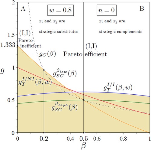
To make Figure 1 (non-network industry, $n=0$) and all the other figures easier to follows, we point out that the feasible region (above the relevant constraints) is white, and the unfeasible region is sand-coloured (below the relevant constraints). The feasible region is divided by a straight vertical black solid line into two areas in which $x_i$ and $x_j$ are strategic substitutes (left of the straight vertical black line) and strategic complements (right of the straight vertical black line). The black dotted line represents the threshold $g_C$, i.e. the locus of point for which $\mathrm{\Delta }{\mathrm{\Pi }}_C=0$. Area A (left of $g_C$) is the parameter space $(\beta ,g)$ such that $\mathrm{\Delta }{\mathrm{\Pi }}_C>0$ (the Nash equilibrium (I,I) is Pareto inefficient, and the game is a prisoner’s dilemma). Area B (right of $g_C$) is the parameter space $(\beta ,g)$ such that $\mathrm{\Delta }{\mathrm{\Pi }}_C<0$ (the Nash equilibrium (I,I) is Pareto efficient, and the game is an anti-prisoner’s dilemma). The relevant constraints of Figure 1, plotted for $n=0$, are the stability condition $g_{SC}^{{\beta }_{low}}(\beta ,n)=g_{SC}^{{\beta }_{low}}(\beta )$ (orange line), which is binding for small values of $\beta$, the R&D cost condition I/NI of the investing firm $g_T^{I/NI}(\beta ,n,w)=g_T^{I/NI}(\beta ,w)$ (red line), which is binding for intermediate values of $\beta$, and the R&D cost condition I/I $g_T^{I/I}(\beta ,n,w)=g_T^{I/I}(\beta ,w)$ (blue line), which is binding for larger values of $\beta$. The stability condition $g_{SC}^{{\beta }_{high}}(\beta ,n)=g_{SC}^{{\beta }_{high}}(\beta )$ (green line) is never binding. The relevant constrains of Figures 2 and 3 are the same, but they are plotted for positive or negative values of $n$.

Figure 2. The R&D investment decision game with network effects and symmetric full compatibility ($k_i=k_j=1$): Nash equilibrium outcomes when $w=0.8$ in the case of positive network externalities $n=0.2$ (Panel A), $n=0.5$ (Panel B) and negative network externalities $n=-0.5$ (Panel C), $n=-1$ (Panel D). The sand-coloured region represents the parametric area of unfeasibility in the $(\beta ,g)$ space. Area A: the R&D game with network externalities and full compatibility is a prisoner’s dilemma. Area B: the R&D game with network externalities and full compatibility is an anti-prisoner’s dilemma (deadlock). The game is a deadlock also in the absence of R&D spillovers ($\beta =0$) for any $n\ge 0.5$.

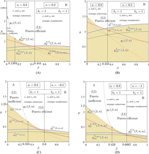
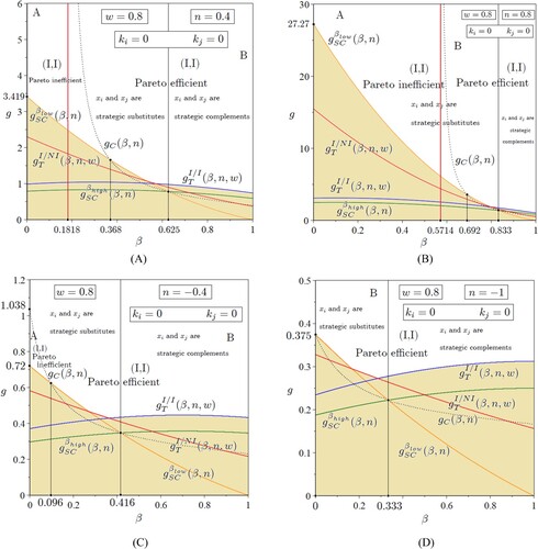
Figure 3. The R&D investment decision game with network effects and symmetric no compatibility ($k_i=k_j=0$): Nash equilibrium outcomes when $w=0.8$ in the case of positive network externalities $n=0.4$ (Panel A), $n=0.8$ (Panel B) and negative network externalities $n=-0.5$ (Panel C), $n=-1$ (Panel D). The sand-coloured region represents the parametric area of unfeasibility in the $(\beta ,g)$ space. Area A: the R&D game with network externalities and no compatibility is a prisoner’s dilemma. Area B: the R&D game with network externalities and no compatibility is an anti-prisoner’s dilemma (deadlock). The game is a deadlock also in the absence of R&D spillovers ($\beta =0$) only when $n=-1$. With positive externalities and symmetric no compatibility, the game is always a prisoner’s dilemma for any $\beta \le \frac{n}{3-2n}$, i.e. for any $\beta \le 0.1818$ if $n=0.4$ and for any $\beta \le 0.5714$ if $n=0.8$ and for any $g$ larger than the relevant binding feasibility condition. If $n=1$, the game is a prisoner’s dilemma for any $0\le \beta \le 1$.

The meaning of the other figures (Figures 2 and 3) is similar though they refer to a network industry with product compatibility. Figure 2 (resp. 3) refers to a network industry under full (resp. no) compatibility.

The SPNE of the game is always (I,I) and the black dotted line $g_C(\beta ,0)=g_C(\beta )$ separates the area (A) in which the Nash equilibrium is Pareto inefficient (low values of $\beta$ and $g$) and the game is a prisoner’s dilemma – self-interest and mutual benefit of cost-reducing innovation conflict –, to the area (B) in which it becomes Pareto efficient (high values of $\beta$ and $g$), and the game is an anti-prisoner’s dilemma (deadlock) – self-interest and mutual benefit do not conflict.

The black dotted line $g_C(\beta )$ and the stability condition $g_{SC}^{{\beta }_{low}}(\beta )$ cross at $\beta =\frac{1}{5}$, corresponding to which $x_i$ and $x_j$ are strategic substitutes, in turn implying that the prisoner’s dilemma cannot be solved in the absence of R&D spillovers. Indeed, the threshold that separates the region in which $x_i$ and $x_j$ are strategic substitutes to the region in which they are strategic complements can be obtained when the stability conditions $g_{SC}^{{\beta }_{low}}(\beta )=g_{SC}^{{\beta }_{high}}(\beta )$ cross at $\beta =\frac{1}{2}$ when $n=0$. Therefore, there is a dominant strategy (I) irrespective of the parameter scale.

However, under the assumption in which the outcome is robust according to a game-theoretic approach (i.e. $\beta =0$) the Nash equilibrium (I,I) is sub-optimal, as firms have a joint incentive to coordinate towards NI, though each of them has a unilateral incentive to play I and invest in R&D. Given the payoff matrix, no one is interested in playing NI if the rival plays NI. This is because everyone prefers to unilaterally invest in process innovation, increase output, and obtain a higher profit.

Also, no one is interested in playing NI, even when the rival plays I. This is because each player prefers to forgo being NI rather than be the only one to play NI, which leads to the worst possible outcome, as a portion of its profits is eroded by the rival that is investing in R&D. Thus, regardless of the rival’s activity, no one will play NI, and everyone will forgo obtaining a higher profit by becoming an investing firm.

However, if both players decide to cooperate in becoming a non-investing firm, they will be better off. Thus, by making decisions that guarantee each player the best outcome unilaterally, both players are worse off than they would have been if they had both chosen to play NI. The pursuit of individual success can thus lead to a collective failure. However, we cannot then expect that both players, aware that they may face disappointment by this result, will reach an agreement to jointly play NI. Players’ choices are consistent if and only if no one should regret them after learning of the rivals’ strategy.

In an R&D game with this parameter configuration, players make consistent decisions when they choose to play I. After both firms have chosen to play I, no one will regret it, as anyone who had decided to play NI unilaterally would have been worse off.

In contrast, players would have made conflicting decisions if they had both chosen to cooperate and play NI. In this case, each would have regretted their choice as playing I unilaterally would have been better off resulting in a higher payoff. On the one hand, we must expect players to be able to achieve an agreement prescribing consistent choices (R&D investments), because everyone is aware that no one after the agreement will be interested in the violation if the rival complies with it. On the other hand, we should not expect players to be able to achieve an agreement prescribing choices that are not mutually consistent (no R&D investment). This is because everyone is aware that no one will be interested in complying with that agreement if the rival complies with it.

The outcomes summarised in Figure 1 ($n=0$) represent a benchmark useful for comparison purposes for any $n\ne 0$ under the assumption of symmetric full compatibility between the two networks ($k_i=k_j=1$), which is studied in this section, and symmetric no compatibility between the two networks ($k_i=k_j=0$), which will be the object of Section 4.

We now move to the analysis of the Nash equilibrium outcomes by considering the existence of positive or negative network externalities with symmetric full compatibility. The role of the R&D cost conditions in defining the feasible region in the parametric space $(\beta ,g)$, and thus their relative position with respect to the stability conditions, depends amongst other things on the unitary technology of production cost $w$.

However, as the nature of the game is a prisoner’s dilemma or deadlock regardless of the relative size of $w$, with I being a dominant strategy, we study the Nash equilibria of the game with symmetric full compatibility by considering the simplest case according to which $w$ is sufficiently high that the stability condition $g_{SC}^{{\beta }_{low}}(\beta ,n)$ is binding when $\beta =0$, and $g_C(\beta ,n)=g_{SC}^{{\beta }_{low}}(\beta ,n)$ when the inequality $g_{SC}^{{\beta }_{low}}(\beta ,n)\ge g_T^{I/NI}(\beta ,n,w)$ holds. This is always verified when $\frac{2}{3}\le w<1$,⁶ which is assumed to be fulfilled henceforth in this section. We pinpoint however that the results presented in this section hold for any $0<w<1$.

We chose to restrict the analysis to the case $w\ge \frac{2}{3}$ as results in this case are easier to handle and interpret than when $w<\frac{2}{3}$. This is because of the role played by the stability and R&D cost conditions in identifying the feasible region, with respect to which $g$ must be sufficiently high to avoid excessive R&D investments, as was explained above.

The following proposition shows the Nash equilibria of the R&D investment decision game with network effects and symmetric full compatibility.

Proposition 3.3:

[Positive externality, $0<n\le 1$].

1. If $0<n<\frac{1}{2}$ then

[1.1] (I,I) is the unique Pareto inefficient Nash equilibrium and the R&D investment decision game with network effects and symmetric full compatibility is a prisoner’s dilemma for any $0\le \beta \le \frac{1-2n}{5-2n}$ and $g_{SC}^{{\beta }_{low}}(\beta ,n)<g<g_C(\beta ,n)$, and [1.2] (I,I) is the unique Pareto efficient Nash equilibrium and the R&D investment decision game with network effects and symmetric full compatibility is an anti-prisoner’s dilemma (deadlock) for any $0\le \beta \le \frac{1-2n}{5-2n}$ and $g>g_C(\beta ,n)$, for any $\frac{1-2n}{5-2n}<\beta \le \frac{w(2-n)-1}{w(2-n)}$ and $g>g_{SC}^{{\beta }_{low}}(\beta ,n)$, for any $\frac{w(2-n)-1}{w(2-n)}<\beta \le \frac{w(1-n)}{1+w(1-n)}$ and $g>g_T^{I/NI}(\beta ,n,w)$, and for any $\frac{w(1-n)}{1+w(1-n)}<\beta \le 1$ and $g>g_T^{I/I}(\beta ,n,w)$.

(2)

If $\frac{1}{2}\le n\le 1$ then (I,I) is the unique Pareto efficient Nash equilibrium and the R&D investment decision game with network effects and symmetric full compatibility is an anti-prisoner’s dilemma for any $0\le \beta \le \frac{w(2-n)-1}{w(2-n)}$ and $g>g_{SC}^{{\beta }_{low}}(\beta ,d)$, for any $\frac{w(2-n)-1}{w(2-n)}<\beta \le \frac{w(1-n)}{1+w(1-n)}$ and $g>g_T^{I/NI}(\beta ,n,w)$, and for any $\frac{w(1-n)}{1+w(1-n)}<\beta \le 1$ and $g>g_T^{I/I}(\beta ,n,w)$.

[Negative externality, $-1\le n<0$].

(3)	If $-1\le n<0$ then

[3.1] (I,I) is the unique Pareto inefficient Nash equilibrium and the R&D investment decision game with network effects and symmetric full compatibility is a prisoner’s dilemma for any $0\le \beta \le \frac{1-2n}{5-2n}$ and $g_{SC}^{{\beta }_{low}}(\beta ,n)<g<g_C(\beta ,n)$, and [3.2] (I,I) is the unique Pareto efficient Nash equilibrium and the R&D investment decision game with network effects and symmetric full compatibility is an anti-prisoner’s dilemma (deadlock) for any $0\le \beta \le \frac{1-2n}{5-2n}$ and $g>g_C(\beta ,n)$, for any $\frac{1-2n}{5-2n}<\beta \le \frac{w(2-n)-1}{w(2-n)}$ and $g>g_{SC}^{{\beta }_{low}}(\beta ,n)$, for any $\frac{w(2-n)-1}{w(2-n)}<\beta \le \frac{w(1-n)}{1+w(1-n)}$ and $g>g_T^{I/NI}(\beta ,n,w)$, and for any $\frac{w(1-n)}{1+w(1-n)}<\beta \le 1$ and $g>g_T^{I/I}(\beta ,n,w)$.

Proof:

See the appendix.

Unlike in the absence of network externalities, the unique SPNE (I,I) can be Pareto efficient also in the absence of R&D spillovers (i.e. no disclosure). This result differs from Bacchiega, Lambertini, and Mantovani (2010) and has some similarities with the R&D game with horizontal product differentiation developed by Buccella, Fanti, and Gori (2021a), who showed that the prisoner’s dilemma can be solved (also in the absence of spillovers) if products are sufficiently differentiated.

Proposition 3.3, which is illustrated in Figure 2 by assuming $w=0.8$, shows that the prisoner’s dilemma can be solved by a sufficiently high extent of positive network effect. The parametric area in the $(\beta ,g)$ space in which the unique SPNE is a prisoner’s dilemma shrinks as $n$ increases. When $n$ becomes sufficiently high, (I,I) is Pareto efficient for any $\beta$, including the case of no disclosure.

This result stresses that investing in R&D in network industries R&D is Pareto superior compared to the case of non-network goods. The intuition is quite smooth. A positive network externality (under full compatibility) shifts leftward the market demand and this, in turn, causes an increase in the quantity produced and sold by both firms as well as an increase in the marginal willingness to pay of consumers (bandwagon effect). Indeed, the network external effects – favouring strategic complementarity – already caused a rise in the cost-reducing R&D effort of both firms, thus making less important R&D disclosure. All these effects tend to increase profits.

4. The R&D investment decision game with network effects and symmetric no compatibility

Let us assume that $k_i=k_j=0$. Like the previous section, the main equilibrium equations of the model with symmetric no compatibility are the following: (25) $x_i^{\ast I/I}(0,0)=\frac{2(1-w)(2-\beta -n)}{g(1-n){(3-n)}^2-2(1+\beta )(2-\beta -n)},$(25) (26) $q_i^{\ast I/I}(0,0)=\frac{g(1-w)(1-n)(3-n)}{g(1-n){(3-n)}^2-2(1+\beta )(2-\beta -n)},$(26) (27) ${\mathrm{\Pi }}_i^{\ast I/I}(0,0)=\frac{g{(1-w)}^2[g{(1-n)}^2{(3-n)}^2-2{(2-\beta -n)}^2]}{{[g(1-n){(3-n)}^2-2(1+\beta )(2-\beta -n)]}^2},$(27) where $g>\frac{2(1+\beta )(2-\beta -n)}{(1-n){(3-n)}^2}:=g_{SC}^{{\beta }_{high}}(\beta ,n)$ (see Equation (37)) must hold to guarantee positive values of R&D effort and production in the subgame I/I, and $g>\frac{2{(2-\beta -n)}^2}{{(1-n)}^2{(3-n)}^2}:=g_{SOC}(\beta ,n)$ must hold to guarantee correspondingly positive profits. These inequalities respectively represent one of the stability conditions and the second-order condition under $(0,0)$, i.e. symmetric no compatibility ($k_i=k_j=0$). In addition, for the symmetric subgame NI/NI and the asymmetric subgame I/NI we have that: (28) $q_i^{\ast NI/NI}(0,0)=\frac{1-w}{3-n},$(28) (29) ${\mathrm{\Pi }}_i^{\ast NI/NI}(0,0)=\frac{{(1-w)}^2}{{(3-n)}^2},$(29) and (30) $x_i^{\ast I/NI}(0,0)=\frac{2(1-w)(1-n)(2-\beta -n)}{g{(1-n)}^2{(3-n)}^2-2{(2-\beta -n)}^2},$(30) (31) $q_i^{\ast I/NI}(0,0)=\frac{g(1-w){(1-n)}^2(3-n)}{g{(1-n)}^2{(3-n)}^2-2{(2-\beta -n)}^2},$(31) (32) $q_j^{\ast I/NI}(0,0)=\frac{(1-w)[g{(1-n)}^2(3-n)-2(1-\beta )(2-\beta -n)]}{g{(1-n)}^2{(3-n)}^2-2{(2-\beta -n)}^2},$(32) (33) ${\mathrm{\Pi }}_i^{\ast I/NI}(0,0)=\frac{g{(1-w)}^2{(1-n)}^2}{g{(1-n)}^2{(3-n)}^2-2{(2-\beta -n)}^2},$(33) (34) ${\mathrm{\Pi }}_j^{\ast I/NI}(0,0)=\frac{{(1-w)}^2{[g{(1-n)}^2(3-n)-2(1-\beta )(2-\beta -n)]}^2}{{[g{(1-n)}^2{(3-n)}^2-2{(2-\beta -n)}^2]}^2},$(34) where $g>g_{SOC}(\beta ,n)$ must hold to guarantee positive values of R&D effort, production and profits of the investing firm $i$, and $g>\frac{2(1-\beta )(2-\beta -n)}{{(1-n)}^2(3-n)}:=g_{SC}^{{\beta }_{low}}(\beta ,n)$ (see Equation (36)) must hold to guarantee positive values of production of the non-investing firm $j$.

In this case, the second-order condition for a maximum requires that the inequality (35) $g>\frac{2{(2-\beta -n)}^2}{{(1-n)}^2{(3-n)}^2}:=g_{SOC}(\beta ,n)(\mathrm{second}\text{-}\mathrm{order}\mathrm{condition}),$(35) must hold to guarantee that the solution is economically meaningful. When $n=0$ this condition boils down to the standard non-network condition, which is identical to the one already presented in the previous section. Regarding the R&D reaction curves in the case of network externalities and symmetric incompatibility we have that $\frac{d{x}_i}{d{x}_j}<0$ if and only if $\beta <\frac{1}{2-n}$ ($x_i$ and $x_j$ are strategic substitutes) and $\frac{d{x}_i}{d{x}_j}>0$ if and only if $\beta >\frac{1}{2-n}$ ($x_i$ and $x_j$ are strategic complements). Definitively, the stability conditions $\left|\frac{d{x}_i}{d{x}_j}\right|<1$ in the R&D model with network externalities and symmetric incompatibility are the following: (36) $g>g_{SC}^{{\beta }_{low}}(\beta ,n)=\frac{2(1+\beta )(2-\beta -n)}{(1-n){(3-n)}^2}\mathrm{if}0\le \beta <\frac{1}{2-n},(x_i\mathrm{and}{x}_j\mathrm{are}\mathrm{strategic}\mathrm{substitutes}),$(36) and (37) $g>g_{SC}^{{\beta }_{high}}(\beta ,n)=\frac{2(1-\beta )(2-\beta -n)}{{(1-n)}^2(3-n)}\mathrm{if}\frac{1}{2-n}<\beta \le 1,(x_i\mathrm{and}{x}_j\mathrm{are}\mathrm{strategic}\mathrm{complements}),$(37) where $g_{SC}^{{\beta }_{low}}(\beta ,n)>g_{SC}^{{\beta }_{high}}(\beta ,n)$ for any $0\le \beta \le \frac{1}{2-n}$ and $g_{SC}^{{\beta }_{low}}(\beta ,n)<g_{SC}^{{\beta }_{high}}(\beta ,n)$ for any $\frac{1}{2-n}\le \beta \le 1$. Also in this case, the second-order condition is always verified if the stability conditions are fulfilled. Combining these results with Equations (25)–(27) allows us to state the following propositions.

Proposition 4.4:

[Positive externality, $0<n\le 1$]. An increase in the strength of the positive network effect ($n\uparrow$) under symmetric incompatibility ($k_i=k_j=0$) increases R&D effort, production and profits in the subgame I/I. [Negative externality, $-1\le n<0$]. An increase in the strength of the negative network effect ($|n|\uparrow$) under symmetric incompatibility ($k_i=k_j=0$) reduces R&D effort, production and profits in the subgame I/I.

Proof:

From Equations (25), (26), and (27) one gets $\frac{d{x}_i^{\ast I/I}(0,0)}{dn}>0$, $\frac{d{q}_i^{\ast I/I}(0,0)}{dn}>0$ and $\frac{d{\mathrm{\Pi }}_i^{\ast I/I}(0,0)}{dn}>0$ for any $-1\le n\le 1$ and for any $g$ satisfying the stability conditions. Q.E.D.

Proposition 4.5:

[Positive externality, $0<n\le 1$]. An increase in the strength of the positive network effect ($n\uparrow$) under symmetric incompatibility ($k_i=k_j=0$) shifts the threshold $\frac{1}{2-n}$ rightward and increases the region of strategic substitutability between $x_i$ and $x_j$ in the $(\beta ,g)$ space. If $n=1$, $\frac{1}{2-n}=1$ and $x_i$ and $x_j$ are strategic substitutes for any $0\le \beta \le 1$. [Negative externality, $-1\le n<0$]. An increase in the strength of the negative network effect ($|n|\uparrow$) under symmetric incompatibility ($k_i=k_j=0$) shifts the threshold $\frac{1}{2-n}$ leftward and increases the region of strategic complementarity between $x_i$ and $x_j$ in the $(\beta ,g)$ space.

Proof:

The proof follows by computing the first order derivative of $\frac{1}{2-n}$ with respect to $n$, which is positive for any $-1\le n\le 1$, noting also that $\frac{1}{2-n}=1$ when $n=1$. Q.E.D.

Proposition 4.4 resembles Proposition 3.1 so that an increase in the strength of the network size positively (resp. negatively) affects, ceteris paribus, R&D effort, production and profits of each firm, though there exists an external effect generated only by the consumers’ expectations about firm $i$’s equilibrium total sales on the demand for the product of network $i$ (given the assumption of symmetric no compatibility). In this case, there are no effects of the demand directed to the rival’s network on the R&D effort of each firm.

The impact of the network externality on the R&D effort under symmetric incompatibility can also be ascertained by considering Proposition 4.5, which pinpoints an opposite role of the network externality on R&D investment with respect to those analysed in Proposition 3.2. Unlike the case of symmetric full compatibility, the positive (resp. negative) network externality favours R&D substitutability (resp. complementarity) and this, in turn, shows the existence of a negative (resp. positive) effect of each firm’s R&D effort on the rival’s one, which indeed generates an indirect negative (resp. positive) effect on the market demand that goes in the opposite direction of the direct effect by reducing (resp. increasing) output and profits. However, the latter effects never overcomes the former.

Under symmetric incompatibility, each firm aims at investing in R&D to increase its own production that, in turn, affects the demand of its own network only without affecting the demand of the rival’s one. This tends to strengthen the substitutability (resp. complementarity) between $x_i$ and $x_j$ in the case of positive (resp. negative) network externalities.

In this regard, an increase in (the absolute value of) $n$ plays the opposite (resp. same) role as an increase in the degree of product differentiation in the R&D investment decision game with non-network-horizontally-differentiated goods. If the intensity of the positive externality is the highest, the threshold $\frac{1}{2-n}$ becomes the highest ($1$) so that $x_i$ and $x_j$ are always strategic substitutes in the feasible region of the $(\beta ,g)$ space. Pairwise, if the intensity of the negative externality is the highest, the threshold $\frac{1}{2-n}$ becomes the lowest ($\frac{1}{3}$) so that the feasible region of the $(\beta ,g)$ space in which $x_i$ and $x_j$ are always strategic complements is the highest.

Like the previous section, we now augment the analysis with the R&D cost conditions emerging from the symmetric and asymmetric subgames. Using (1) the inequality $w-x_i-\beta x_j>0$ together with Equation (25) for the symmetric subgame I/I, and (2) the inequality $w-x_i>0$ referred to the investing firm $i$ in the asymmetric subgame I/NI together with Equation (30) one gets (38) $g>\frac{2(1+\beta )(2-\beta -n)}{w(1-n){(3-n)}^2}:=g_T^{I/I}(\beta ,n,w),(\mathrm{R}\mathrm{\&}\mathrm{D}\mathrm{cost}\mathrm{condition}\mathrm{I}/\mathrm{I}),$(38) and (39) $g>\frac{2(2-\beta -n)[1-n+w(1-\beta )]}{w{(1-n)}^2{(3-n)}^2}:=g_T^{I/NI}(\beta ,n,w),(\mathrm{R}\mathrm{\&}\mathrm{D}\mathrm{cost}\mathrm{condition}\mathrm{I}/\mathrm{NI}).$(39)

At the first stage of the game firms choose whether to invest in R&D in a non-cooperative quantity-setting environment à la AJ augmented with network effects and symmetric no compatibility. Using Equations (27), (29), (33) and (34), we can construct the payoff matrix summarised in Table 2.

Table 2. The investment-decision game with network effects and $k_i=k_j=0$ (payoff matrix).

Firm $i$ ↓ Firm $j$ →	I	NI
I	${\mathrm{\Pi }}_i^{\ast I/I}(0,0)$, ${\mathrm{\Pi }}_j^{\ast I/I}(0,0)$	${\mathrm{\Pi }}_i^{\ast I/NI}(0,0)$, ${\mathrm{\Pi }}_j^{\ast I/NI}(0,0)$
NI	${\mathrm{\Pi }}_i^{\ast NI/I}(0,0)$, ${\mathrm{\Pi }}_j^{\ast NI/I}(0,0)$	${\mathrm{\Pi }}_i^{\ast NI/NI}(0,0)$, ${\mathrm{\Pi }}_j^{\ast NI/NI}(0,0)$

As usual, the analysis is restricted to let the feasibility constraints being satisfied. Under the assumption of no compatibility $k_i=k_j=0$, the inequalities presented in (36)–(39) must hold. Then, to derive all of the possible equilibria of the game, one must study the sign of the profit differentials $\mathrm{\Delta }{\mathrm{\Pi }}_A(0,0):={\mathrm{\Pi }}_i^{\ast I/NI}(0,0)-{\mathrm{\Pi }}_i^{\ast NI/NI}(0,0)$, $\mathrm{\Delta }{\mathrm{\Pi }}_B(0,0):={\mathrm{\Pi }}_i^{\ast NI/I}(0,0)-{\mathrm{\Pi }}_i^{\ast I/I}(0,0)$ and $\mathrm{\Delta }{\mathrm{\Pi }}_C(0,0):={\mathrm{\Pi }}_i^{\ast NI/NI}(0,0)-{\mathrm{\Pi }}_i^{\ast I/I}(0,0)$ for $i=\{1,2\},i\ne j$. Under the assumption of symmetric no compatibility we have that $\mathrm{\Delta }{\mathrm{\Pi }}_A(0,0)>0$ and $\mathrm{\Delta }{\mathrm{\Pi }}_B(0,0)<0$, irrespective of the parameter scale, whereas $\mathrm{\Delta }{\mathrm{\Pi }}_C(0,0)$ can be positive or negative depending on the relative values of $\beta$, $g$ and $n$.

In this regard, we have that $sgn\{\mathrm{\Delta }{\mathrm{\Pi }}_C(0,0)\}=sgn\{-g{(3-n)}^2[\beta (3-2n)-n]+2{(1+\beta )}^2(2-\beta -n)\}$.

If $n>0$ and $\beta \le \frac{n}{3-2n}$ then $\mathrm{\Delta }{\mathrm{\Pi }}_C(0,0)>0$ for any $g$ belonging to the feasible region in the $(\beta ,g)$ space and profits of both firms under the strategic profile NI/NI are higher than under the strategic profile I/I.

If $n>0$ and $\beta >\frac{n}{3-2n}$ then $\mathrm{\Delta }{\mathrm{\Pi }}_C(0,0)>0$ for any $g<g_C(\beta ,n)$ and profits of both firms under the strategic profile NI/NI are higher than under the strategic profile I/I, and $\mathrm{\Delta }{\mathrm{\Pi }}_C(0,0)<0$ for any $g>g_C(\beta ,n)$ and profits of both firms under the strategic profile I/I are higher than under the strategic profile NI/NI, where (40) $g_C(\beta ,n):=\frac{2{(1+\beta )}^2(2-\beta -n)}{{(3-n)}^2[\beta (3-2n)-n]},$(40) is the threshold value of $g$ as a function of the intensity of the R&D spillovers and the degree of network effect such that $\mathrm{\Delta }{\mathrm{\Pi }}_C(0,0)=0$. An increase in the degree of network effects in the case of positive externalities not only increases the region of strategic substitutability between $x_i$ and $x_j$ in the parametric space $(\beta ,g)$, as shown in Proposition 4.5, but also contributes to shift the threshold $\frac{n}{3-2n}$ rightward in turn broadening the space in which $\mathrm{\Delta }{\mathrm{\Pi }}_C(0,0)>0$.

If $n<0$, then $\mathrm{\Delta }{\mathrm{\Pi }}_C(0,0)>0$ for any $g<g_C(\beta ,n)$ and profits of both firms under the strategic profile NI/NI are higher than under the strategic profile I/I, and $\mathrm{\Delta }{\mathrm{\Pi }}_C(0,0)<0$ for any $g>g_C(\beta ,n)$ and profits of both firms under the strategic profile I/I are higher than under the strategic profile NI/NI.

Mirroring the analysis of the previous section, we now turn to the study of the Nash equilibrium outcomes of the game under the assumption of no compatibility. In doing so, we continue to assume that the condition $\frac{2}{3}\le w<1$ is satisfied to simplify the narrative in defining the feasible region in the parametric space $(\beta ,g)$, though the qualitative results detailed in the following proposition hold irrespective of the size of $w$. First, we pinpoint that $w>\frac{1-n}{2-n}$ for any $\frac{2}{3}\le w<1$ and $-1\le n\le 1$.

Proposition 4.6:

[Positive externality, $0<n\le 1$].

1. If $0<n<1$ and $\beta \le \frac{n}{3-2n}$ then (I,I) is the unique Pareto inefficient Nash equilibrium and the R&D investment decision game with network effects and symmetric no compatibility is a prisoner’s dilemma for any $0\le \beta \le \frac{n}{3-2n}$ and $g>g_{SC}^{{\beta }_{low}}(\beta ,n)$.

2. If $0<n<1$ and $\beta >\frac{n}{3-2n}$ then:

[2.1] (I,I) is the unique Pareto inefficient Nash equilibrium and the R&D investment decision game with network effects and symmetric no compatibility is a prisoner’s dilemma for any $0\le \beta \le \frac{1+n}{5-3n}$ and $g_{SC}^{{\beta }_{low}}(\beta ,n)<g<g_C(\beta ,n)$, and [2.2] (I,I) is the unique Pareto efficient Nash equilibrium and the R&D investment decision game with network effects and symmetric no compatibility is an anti-prisoner’s dilemma (deadlock) for any $0\le \beta \le \frac{1+n}{5-3n}$ and $g>g_C(\beta ,n)$, for any $\frac{1+n}{5-3n}<\beta \le \frac{w(2-n)-(1-n)}{w(2-n)}$ and $g>g_{SC}^{{\beta }_{low}}(\beta ,n)$, for any $\frac{w(2-n)-(1-n)}{w(2-n)}<\beta \le \frac{w}{1-n+w}$ and $g>g_T^{I/NI}(\beta ,n,w)$, and for any $\frac{w}{1-n+w}<\beta \le 1$ and $g>g_T^{I/I}(\beta ,n,w)$.

(3)	If $n=1$ then (I,I) is the unique Pareto inefficient Nash equilibrium and the R&D investment decision game with network effects and symmetric no compatibility is a prisoner’s dilemma for any $0\le \beta \le 1$ and $g>g_{SC}^{{\beta }_{low}}(\beta ,n)$.

[Negative externality, $-1\le n<0$].

(4)	If $-1<n<0$ then:

[4.1] (I,I) is the unique Pareto inefficient Nash equilibrium and the R&D investment decision game with network effects and symmetric no compatibility is a prisoner’s dilemma for any $0\le \beta \le \frac{1+n}{5-3n}$ and $g_{SC}^{{\beta }_{low}}(\beta ,n)<g<g_C(\beta ,n)$, and [4.2] (I,I) is the unique Pareto efficient Nash equilibrium and the R&D investment decision game with network effects and symmetric no compatibility is an anti-prisoner’s dilemma (deadlock) for any $0\le \beta \le \frac{1+n}{5-3n}$ and $g>g_C(\beta ,n)$, for any $\frac{1+n}{5-3n}<\beta \le \frac{w(2-n)-(1-n)}{w(2-n)}$ and $g>g_{SC}^{{\beta }_{low}}(\beta ,n)$, for any $\frac{w(2-n)-(1-n)}{w(2-n)}<\beta \le \frac{w}{1-n+w}$ and $g>g_T^{I/NI}(\beta ,n,w)$, and for any $\frac{w}{1-n+w}<\beta \le 1$ and $g>g_T^{I/I}(\beta ,n,w)$.

(5)

If $n=-1$ then (I,I) is the unique Pareto efficient Nash equilibrium and the R&D investment decision game with network effects and symmetric no compatibility is an anti-prisoner’s dilemma for any $0\le \beta \le \frac{w(2-n)-(1-n)}{w(2-n)}$ and $g>g_{SC}^{{\beta }_{low}}(\beta ,d)$, for any $\frac{w(2-n)-(1-n)}{w(2-n)}<\beta \le \frac{w}{1-n+w}$ and $g>g_T^{I/NI}(\beta ,n,w)$, and for any $\frac{w}{1-n+w}<\beta \le 1$ and $g>g_T^{I/I}(\beta ,n,w)$.

Proof:

See the appendix.

Proposition 4.6 – whose geometric projection is depicted in Figure 3 – shows that when the network externality affects only products of the network in which the firm is engaged (no compatibility), (1) the parametric area in which (I,I) the prisoner’s dilemma increases as the extent of the network effect becomes larger in the space $(\beta ,g)$ under positive externality. This is the opposite of the results of Proposition 3.3 analysed so far and Buccella, Fanti, and Gori (2021a), i.e. as far as the spill-over rate decreases it is less likely to solve the dilemma as $n$ increases. For example, if $n=0$ (Bacchiega, Lambertini, and Mantovani 2010) the necessary condition to solve the dilemma ($\beta \ge \frac{1+n}{5-3n}$) is $\beta \ge 0.2$; if $n=0.4$ (resp. $n=0.8$) this condition becomes $\beta \ge 0.368$ (resp. $\beta \ge 0.692$). As $n$ tends to $1$ the prisoner’s dilemma becomes the sole paradigm for any $0\le \beta \le 1$. For clarity, we pinpoint that, unlike the previous figures, Figure 3 (Panel A and Panel B) depicts a straight vertical red solid line that separates the region in which the game is always a prisoner’s dilemma (left) to the region in which the threshold $g_C$ is binding (right), so that the game is a prisoner’s (resp. anti-prisoner’s) dilemma for any couple $(\beta ,g)$ below (resp. above) the dotted line.

When $k_i=0$ there is no network effect on the rival’s demand, and thus investing in R&D for firm $j$ leads to a cost reduction causing a substantial increase in output, thus implying a reduction in the marginal willingness to pay of consumers that, in turn, contributes to reduce its profits. Differently, when $k_i=1$, there is network effect on the rival’s demand, and thus firm $i$’s output supports the rival’s demand as well as the price of firm $j$ to the extent that this (positive) effect outweighs the negative one due to the R&D-induced increase in output that, in turn, causes a reduction in price.

Definitively, Propositions 3.3 and 4.6 summarise the outcomes of two polar cases. Indeed, if there is symmetric incompatibility the network effect acts only for one’s own product. On one hand, this increases the incentive of carrying on R&D unilaterally; however, on the other hand, when both firms invest in R&D, the effect of the increase in quantity is exacerbated (compared to the case with no network, i.e. $n=0$), and thus profits in equilibrium are lower than in the absence of R&D. If there is full compatibility the demand to each firm (and its profits) increases along with the quantity produced by the rival. Therefore, the R&D investment, by reducing costs and increasing output, causes a net beneficial effect on profits as the output increase of each firm also contributes to increase the rival’s demand to the point in which profits under R&D are higher than profits under no R&D, even in the absence of spillovers.

The results discussed so far can be extended to the case of symmetric imperfect compatibility, $k_i=k_j=k$ (see the online Appendix for a discussion on the different stages of the game to compute best replies and the optimal values of quantities and R&D investments in the various subgames). Following the usual assumption $\frac{2}{3}\le w<1$, the R&D investment decision game with network externality and compatibility (I versus NI) continues to be a prisoner’s dilemma or an anti-prisoner’s dilemma for any values of $\beta$ and $g$ belonging to the feasible region, in which there exists a dominant strategy (I), and (I,I) is the unique sub-game perfect Nash equilibrium in pure strategies. This extension is interesting as it allows to pinpoint the role of the network strength ($n$) and the extent of degree of product compatibility ($k$) in determining a bifurcation from a prisoner’s to an anti-prisoner’s dilemma in the parameter space $(\beta ,g)$, which is used for comparison purposes with the case $n=0$. Of course, the network strength affects the economy irrespective of whether products are perfectly or imperfectly in(compatible), but the degree of product compatibility is strictly related to existence of network externalities.

The main outcomes of the game I versus NI with $k>0$ can be found by studying the sign of $\mathrm{\Delta }{\mathrm{\Pi }}_C(k,k)$, which can be positive or negative depending on the relative values of $\beta$, $g$, $n$ and $k$. In this regard, we have that $sgn\{\mathrm{\Delta }{\mathrm{\Pi }}_C(k,k)\}=sgn\{-g{[3-n(1+k)]}^2\{\beta [3-n(2-k)]-n(1-2k)\}+2{(1+\beta )}^2[2-\beta -n(1-k\beta )]\}$. The threshold $\mathrm{\Delta }{\mathrm{\Pi }}_C(k,k)=0$ holds if and only if $g=g_C(\beta ,n,k):=\frac{2{(1+\beta )}^2[2-\beta -n(1-\beta k)]}{{[3-n(1+k)]}^2\{\beta [3-n(2-k)]-n(1-2k)\}}$, which should be compared with the stability condition $g_{SC}^{{\beta }_{low}}(\beta ,n,k):=\frac{2(1-\beta )[2-\beta -n(1-\beta k)]}{{[1-n(1-k)]}^2[3-n(1+k)]}$. Results are divided in four cases.

• Scenario 1: $n>0$ and $k\ge \frac{1}{2}$. In this case, $\mathrm{\Delta }{\mathrm{\Pi }}_C(k,k)>0$ for any $g<g_C(\beta ,n,k)$ and $\mathrm{\Delta }{\mathrm{\Pi }}_C(k,k)<0$ for any $g>g_C(\beta ,n,k)$. The former (resp. latter) holds for sufficiently low (resp. high) values of $\beta$ and $g$ belonging to the feasible region (i.e. satisfying the relevant constraints). Then, the game is a prisoner’s (resp. anti-prisoner’s) dilemma and (I,I) is the Nash equilibrium. In this scenario, there exists a value of $n=\frac{1}{3k-1}$, which is decreasing in $k$, that solves the dilemma for any $0\le \beta \le 1$ if and only if $\frac{2}{3}\le k\le 1$. This value can be obtained by setting $g_{SC}^{{\beta }_{low}}(\beta ,n,k)=g_C(\beta ,n,k)$ and solving for $n$. If $\frac{1}{2}\le k<\frac{2}{3}$, the prisoner’s dilemma is solved only for positive values of $\beta$. The case of full compatibility belong to this scenario.

• Scenario 2: $n>0$ and $k<\frac{1}{2}$. If $\beta >\frac{n(1-2k)}{3-n(2-k)}$ then $\mathrm{\Delta }{\mathrm{\Pi }}_C(k,k)>0$ for any $g<g_C(\beta ,n,k)$ and $\mathrm{\Delta }{\mathrm{\Pi }}_C(k,k)<0$ for any $g>g_C(\beta ,n,k)$. In this case, the outcomes of the game are the same as those in Scenario 1, but a value of $n$ solving the dilemma for any $0\le \beta \le 1$ and $g$ belonging to the feasible region does never exist. This implies that the prisoner’s dilemma cannot be solved irrespective of the parameter scale. If $\beta <\frac{n(1-2k)}{3-n(2-k)}$ then $\mathrm{\Delta }{\mathrm{\Pi }}_C(k,k)>0$ and the Nash equilibrium (I,I) of the game I versus NI is always Pareto inefficient (prisoner’s dilemma).

Following Scenarios 1 and 2, the policy message when the network externality is positive is clear: high values the degree of compatibility ($\frac{2}{3}\le k\le 1$) favour the solution of the prisoner’s dilemma irrespective of the parameter scale, i.e. for any for any $0\le \beta \le 1$ and $g$ belonging to the feasible region. The lowest possible value of $n$ ($n=\frac{1}{2}$) that solves the prisoner's dilemma occurs when $k=1$; intermediate values of the degree of compatibility ($\frac{1}{2}\le k<\frac{2}{3}$) unavoidably require a positive spill-over to solve the dilemma; lower values of the degree of compatibility ($0\le k<\frac{1}{2}$) unavoidably require a positive spill-over to solve the dilemma but make the spill-over parameter playing a more articulated role. If $\beta$ is above a given threshold, the game is a prisoner’s dilemma for relatively low values of $\beta$ and $g$ belonging to the feasible region and an anti-prisoner’s dilemma for relatively high values of $\beta$ and $g$ belonging to the feasible region. If $\beta$ is below a given threshold, the game is always a prisoner’s dilemma. Therefore, low values the degree of compatibility, including the case of perfect incompatibility, relegate the game I versus NI to be a prisoner’s dilemma irrespective of the parameter scale.

• Scenario 3: $n<0$ and $k\le \frac{1}{2}$. In this case, $\mathrm{\Delta }{\mathrm{\Pi }}_C(k,k)>0$ for any $g<g_C(\beta ,n,k)$ and $\mathrm{\Delta }{\mathrm{\Pi }}_C(k,k)<0$ for any $g>g_C(\beta ,n,k)$. The former (resp. latter) holds for sufficiently low (resp. high) values of $\beta$ and $g$ belonging to the feasible region. Then, the game is a prisoner’s (resp. anti-prisoner’s) dilemma and (I,I) is the Nash equilibrium. In this scenario, however, the unique value of the network strength that solves the dilemma irrespective of the parameter scale is $n=-1$ obtained when $k=0$. If $0<k\le \frac{1}{2}$, the game is a prisoner’s (resp. anti-prisoner’s) dilemma for low, but positive, (resp. high) values of $\beta$ and $g$ belonging to the feasible region. The case of no compatibility belong to this scenario.

• Scenario 4: $n<0$ and $k>\frac{1}{2}$. If $\beta >\frac{n(1-2k)}{3-n(2-k)}$ then $\mathrm{\Delta }{\mathrm{\Pi }}_C(k,k)>0$ for any $g<g_C(\beta ,n,k)$ and $\mathrm{\Delta }{\mathrm{\Pi }}_C(k,k)<0$ for any $g>g_C(\beta ,n,k)$. In this case, the outcomes of the game are the same as those in Scenario 3, but a value of $n$ solving the dilemma for any $0\le \beta \le 1$ and $g$ belonging to the feasible region does never exist. This implies that the prisoner’s dilemma cannot be solved irrespective of the parameter scale. If $\beta <\frac{n(1-2k)}{3-n(2-k)}$ then $\mathrm{\Delta }{\mathrm{\Pi }}_C(k,k)>0$ and the Nash equilibrium (I,I) of the game I versus NI is always Pareto inefficient (prisoner’s dilemma).

Following Scenarios 3 and 4, the policy message when the network externality is negative is clear: the prisoner’s dilemma can be solved only when the externality is at its maximum strength and the degree of compatibility is null. In this case, the anti-compatibility of products helps solving the problem. A positive but low degree of compatibility ($0<k\le \frac{1}{2}$) relegate the solution of the dilemma to positive and high values of $\beta$ and $g$. Larger values of the degree of compatibility ($\frac{1}{2}\le k\le 1$) disfavour the solution of the dilemma by widening the parameter region in the $(\beta ,g)$ space in which the game is always a prisoner’s dilemma.

5. Comparison of equilibrium outcomes between full compatibility and no compatibility

This section aims at comparing the main equilibrium outcomes of the models with full compatibility and no compatibility studied in Sections 3 and 4, respectively. In this regard, the following proposition shows the beneficial effects of full product compatibility for both firms and the society. Before making this point, however, we introduce the definition of consumers’ surplus (which is part of social welfare) at the equilibrium in the cases of full compatibility and no compatibility. In the former case ($k_i=k_j=1$), the market demand for network $i$ (if consumers have rational expectations) is $p_i=1-q_i-q_j+n(q_i+q_j)$. Therefore, the consumers’ surplus and producers’ surplus at the equilibrium are respectively given by $C{S}^{\ast }(1,1):=2(1-n)[q_i^{\ast I/I}(1,1){]}^2$ and $P{S}^{\ast }(1,1):=2{\mathrm{\Pi }}_i^{\ast I/I}(1,1)$ so that social welfare is (41) $W^{\ast }(1,1)=C{S}^{\ast }(1,1)+P{S}^{\ast }(1,1)$(41) In the latter case ($k_i=k_j=0$), the market demand for network $i$ (if consumers have rational expectations) is $p_i=1-q_i-q_j+n{q}_i$. Therefore, the consumers’ surplus and producers’ surplus at the equilibrium are respectively given by $C{S}^{\ast }(0,0):=(2-n)[q_i^{\ast I/I}(0,0){]}^2$ and $P{S}^{\ast }(0,0):=2{\mathrm{\Pi }}_i^{\ast I/I}(0,0)$ so that social welfare in this case is (42) $W^{\ast }(0,0)=C{S}^{\ast }(0,0)+P{S}^{\ast }(0,0)$(42)

Proposition 5.7:

[Positive externality, $0<n\le 1$]. The equilibrium quantity, profits and social welfare under full compatibility are larger than the corresponding values under no compatibility. The equilibrium R&D investment under full compatibility is smaller than the corresponding value under no compatibility. [Negative externality, $-1\le n<0$]. The equilibrium quantity, profits and social welfare under full compatibility are smaller than the corresponding values under no compatibility. The equilibrium R&D investment under full compatibility is larger than the corresponding value under no compatibility.

Proof:

The proof is obvious by direct comparison of (9) and (25), (10) and (26), (11) and (27), and (41) and (42). Q.E.D.

Proposition 5.7 shows the beneficial effect for firms and society of fostering full (resp. no) compatibility under positive (resp. negative) network effects to benefit from the advantages (to contain the disadvantages) of the related positive (resp. negative) externalities on the consumers’ side. Indeed, firms invest in R&D at least as much as in the absence of network externalities. This result is quite intuitive. When there are no network externalities, firms benefit from its R&D investment only through the reduction of its cost of production (with or without disclosure). However, when the consumer’s utility depends on the number of users of perfectly compatible (resp. incompatible) products, there is a higher (resp. lower) need to invest in R&D in the case of positive (resp. negative) externalities compared with the absence of network. This is because of the external effect played by the network in fostering (resp. reducing) the demand for the product of network $i$, which, in turn, causes an additional positive (resp. negative) effect on its profits, so that each firm increases (resp. reduces) its R&D effort also causing a fall (an increase) in the cost of production. The network effect on the demand side generates a fall (resp. increase) in the price of the product and this in turn implies an increase (resp. reduction) in the market demand following an increase in the network size in the case of positive (resp. negative) externalities. All firms benefit (are harmed) equally when products are perfectly compatible (resp. incompatible).

6. R&D subsidies (or taxes) and network externalities

This section aims at complementing the analysis made so far with some policy prescriptions. The main results of the R&D game with network externalities (with full or no compatibility) are related to the solution of the prisoner’s dilemma emerging in Bacchiega, Lambertini, and Mantovani (2010) irrespective of the parameter scale. This opens the route to policies that favour product compatibility as social welfare under I/I is larger than social welfare under NI/NI in both cases of full and no compatibility. This may require designing an ad hoc public incentive towards network effects, which should therefore be carried out by the firm in addition to the R&D effort by endogenizing $n$. This kind of policy, however, may be difficult to implement as network externalities are close to marketing strategies related to customers’ preferences. Indeed, it requires identifying several product characteristics and information that may be costly for the public authority. Alternatively, a policy instrument that can be used as a welfare-maximising tool in this environment is represented by the standard R&D subsidy aimed at incentivising the private R&D effort along the line of Hinloopen (1997), Hinloopen (2000) and Amir et al. (2019). Interestingly, this instrument does not change the nature of the R&D investment decision game with network externalities (which continues to be a deadlock with investing firms irrespective of the parameter scale in either case of exogenous and optimal subsidy) and the role of product differentiation in the model. Therefore, in what follows, we briefly present the structure of the R&D incentive scheme in the subgame I/I and compare the welfare outcomes. Unlike the results of the received literature, we pinpoint that in the case of symmetric no compatibility (as well as in the case of symmetric imperfect compatibility, see the Appendix) the government can maximise social welfare by levying a tax to disincentivise the firm R&D effort or, like the results of the received literature, providing a subsidy to incentivise the firm R&D effort. This depends on the strength of the network effect.

The public policy to incentivise (or disincentivise) the firm R&D effort directly follows the model of Amir et al. (2019), showing that network effects play a relevant role in affecting the optimal R&D policy in both cases of full and no compatibility.

From a modelling perspective, we assume that the R&D subsidies (resp. taxes) towards firm $i$ and firm $j$ are respectively given by ${\mathrm{\Sigma }}_i>0$ and ${\mathrm{\Sigma }}_j>0$ (resp. ${\mathrm{\Sigma }}_i<0$ and ${\mathrm{\Sigma }}_j<0$). The subsidies (resp. taxes) are financed at a balanced budget with a uniform non-distorting lump-sum tax $T>0$ (resp. are used to finance at a balanced budget a uniform non-distorting lump-sum subsidy $T<0$) on the side of consumers.

The available post-tax (resp. post-subsidy) exogenous nominal income of the representative consumer $M-T>0$ is high enough to avoid corner solutions. Therefore, the government budget constraint reads as follows: (43) $T={\mathrm{\Sigma }}_i+{\mathrm{\Sigma }}_j,$(43) where ${\mathrm{\Sigma }}_i=\sigma \frac{g}{2}{x}_i^2$, ${\mathrm{\Sigma }}_j=\sigma \frac{g}{2}{x}_j^2$ and $0\le \sigma <1$ (resp. $-1<\sigma \le 0$) is the subsidy (resp. tax) rate. Definitively, the government first announces the policy, and then let firms be engaged in the R&D investment decision game discussed so far. Results are shown analytically for the cases of symmetric full compatibility and symmetric no compatibility. The case of symmetric partial compatibility ($k_i=k_j=k$) is shown in the appendix (see Proposition A1).

From Equation (5), firm $i$’s profits in the I/I sub-game become: (44) ${\mathrm{\Pi }}_i^{I/I}=[1-q_i-q_j+n(y_i+k_i{y}_j)-w+x_i+\beta x_j]q_i-\frac{g}{2}{x}_i^2(1-\sigma ),i,j=\{1,2\},i\ne j.$(44) Symmetric full (resp. no) compatibility holds when $k_i=k_j=1$ (resp. $k_i=k_j=0$). Once one gets the main equilibrium outcome of the subgame, social welfare at the equilibrium can be computed as $W^{\ast I/I}=C{S}^{\ast I/I}+P{S}^{\ast I/I}-T^{\ast I/I}$. The equilibrium values of R&D investment, quantity and profit with government intervention in the cases $k_i=k_j=1$, $k_i=k_j=0$ and $k_i=k_j=k$ are in the Appendix.

The analysis of $W^{\ast I/I}$ in the two cases leads to the following proposition. A notational clarification: in what follows we will define the social welfare in the cases of symmetric full compatibility and symmetric no compatibility as $W^{\ast I/I}(1,1,\sigma )=C{S}^{\ast I/I}(1,1,\sigma )+P{S}^{\ast I/I}(1,1,\sigma )-T^{\ast I/I}(1,1,\sigma )$ and $W^{\ast I/I}(0,0,\sigma )=C{S}^{\ast I/I}(0,0,\sigma )+P{S}^{\ast I/I}(0,0,\sigma )-T^{\ast I/I}(0,0,\sigma )$, respectively.

Proposition 6.8:

[Optimal policy]. In a Cournot duopoly with network effects, there exists a welfare-maximising policy (subsidies or taxes) towards R&D, which is designed as follows.

[Symmetric full compatibility]. Introducing R&D subsidies in markets with network externalities and symmetric full compatibility is welfare improving, and there exists an optimal subsidy if and only if: (45) $\sigma ={\sigma }^{OPT(1,1)}(n):=\frac{(3-2n)\beta }{(2-n)(1+\beta )}<1,$(45) where (1) ${\sigma }^{OPT(1,1)}(n)>0$ for any $0<\beta \le 1$ and $-1\le n\le 1$, (2) ${\sigma }^{OPT(1,1)}(n)=0$ if $\beta =0$ for any $-1\le n\le 1$, and (3) ${\sigma }^{OPT(1,1)}(n)$ is a monotonic decreasing function of $n$ for any $0<\beta \le 1$.

[Symmetric no compatibility]. Introducing R&D subsidies (or taxes) in markets with network externalities and symmetric no compatibility is welfare improving depending on the extent of the network strength, and there exists an optimal subsidy (tax) if and only if: (46) $\sigma =|{\sigma }^{OPT(0,0)}(n)|:=\frac{(3-n)[2\beta -n(1+\beta )]}{(1-n)(4-n)(1+\beta )}<1,$(46) where (1) ${\sigma }^{OPT(0,0)}(n)>0$ (resp. $<0$) for any $-1\le n<\frac{2\beta }{1+\beta }$ (resp. $\frac{2\beta }{1+\beta }<n\le 1$) and $0<\beta \le 1$, (2) ${\sigma }^{OPT(0,0)}(n)=\frac{-n(3-n)}{(1-n)(4-n)}>0$ (resp. $<0$) for any $n<0$ (resp. $n>0$) if $\beta =0$, and (3) ${\sigma }^{OPT(0,0)}(n)$ is a monotonic decreasing function of $n$ for any $0\le \beta \le 1$.

Proof:

Let $k_i=k_j=1$ hold. Then, by differentiating $W^{\ast I/I}(1,1,\sigma )$ with respect to $\sigma$ one gets: (47) ${\frac{\mathrm{\partial }{W}^{\ast I/I}(1,1,\sigma )}{\mathrm{\partial }\sigma }|}_{\sigma =0}=\frac{8g^2{(1-w)}^2{(3-2n)}^3\beta [1+(1-\beta )(1-n)]}{{\{g{(3-2n)}^2-2(1+\beta )[1+(1-\beta )(1-n)]\}}^3}>0,$(47) for any $g_{SC}^{{\beta }_{high}}(\beta ,n)$, and (48) $\frac{\mathrm{\partial }{W}^{\ast I/I}(1,1,\sigma )}{\mathrm{\partial }\sigma }=\frac{8g^2{(1-w)}^2{(3-2n)}^2[1+(1-\beta )(1-n)][(3-2n)\beta -\sigma (2-n)(1+\beta )]}{{\{g{(3-2n)}^2(1-\sigma )-2(1+\beta )[1+(1-\beta )(1-n)]\}}^3}.$(48) Then, $\frac{\mathrm{\partial }{W}^{\ast I/I}(1,1,\sigma )}{\mathrm{\partial }\sigma }=0$ if and only if $\sigma ={\sigma }^{OPT(1,1)}(n)$. Therefore, $\frac{\mathrm{\partial }{W}^{\ast I/I}(1,1,\sigma )}{\mathrm{\partial }\sigma }>0$ if $\sigma <{\sigma }^{OPT(1,1)}(n)$ and $\frac{\mathrm{\partial }{W}^{\ast I/I}(1,1,\sigma )}{\mathrm{\partial }\sigma }<0$ if $\sigma >{\sigma }^{OPT(1,1)}(n)$ for any $g>\frac{g_{SC}^{{\beta }_{high}}(\beta ,n)}{1-\sigma }$. Point 1 immediately follows from (45). Point 2 follows from (45) by setting $\beta =0$. Point 3 follows by computing $\frac{\mathrm{\partial }{\sigma }^{OPT(1,1)}(n)}{\mathrm{\partial }n}=\frac{-\beta }{{(2-n)}^2(1+\beta )}<0$ for any $0<\beta \le 1$.

Now, let $k_i=k_j=0$ hold. Then, by differentiating $W^{\ast I/I}(0,0,\sigma )$ with respect to $\sigma$ one gets: (49) ${\frac{\mathrm{\partial }{W}^{\ast I/I}(0,0,\sigma )}{\mathrm{\partial }\sigma }|}_{\sigma =0}=\frac{4g^2{(1-w)}^2(1-n){(3-n)}^3(2-\beta -n)[2\beta -n(1+\beta )]}{{[g(1-n){(3-n)}^2-2(1+\beta )(2-\beta -n)]}^3}.$(49) The expression in (49) is positive (resp. negative), and the introduction of an ad hod R&D subsidy (resp. tax) is welfare improving, if and only if $-1\le n<\frac{2\beta }{1+\beta }$ (resp. $\frac{2\beta }{1+\beta }<n\le 1$) for any $g_{SC}^{{\beta }_{high}}(\beta ,n)$. Additionally, one can get: (50) $\frac{\mathrm{\partial }{W}^{\ast I/I}(0,0,\sigma )}{\mathrm{\partial }\sigma }=\frac{4g^2{(1-w)}^2(1-n){(3-n)}^2(2-\beta -n)\{(3-n)[2\beta -n(1+\beta )]-\sigma (1-n)(4-n)(1+\beta )\}}{{[g(1-n){(3-n)}^2(1-\sigma )-2(1+\beta )(2-\beta -n)]}^3}.$(50) Then, $\frac{\mathrm{\partial }{W}^{\ast I/I}(0,0,\sigma )}{\mathrm{\partial }\sigma }=0$ if and only if $\sigma =|{\sigma }^{OPT(0,0)}(n)|$. Therefore, $\frac{\mathrm{\partial }{W}^{\ast I/I}(0,0,\sigma )}{\mathrm{\partial }\sigma }>0$ if $\sigma <|{\sigma }^{OPT(0,0)}(n)|$ and $\frac{\mathrm{\partial }{W}^{\ast I/I}(0,0,\sigma )}{\mathrm{\partial }\sigma }<0$ if $\sigma >|{\sigma }^{OPT(0,0)}(n)|$ for any $g>\frac{g_{SC}^{{\beta }_{high}}(\beta ,n)}{1-\sigma }$. Point 1 immediately follows from (46). Point 2 follows from (46) by setting $\beta =0$. Point 3 follows by computing $\frac{\mathrm{\partial }{\sigma }^{OPT(0,0)}(n)}{\mathrm{\partial }n}=\frac{-2[2+{(2-n)}^2-\beta (5-2n)]}{{(1-n)}^2{(4-n)}^2(1+\beta )}<0$ for any $-1\le n\le 1$ and $0\le \beta \le 1$ as the expression in brackets in the numerator is always positive. Q.E.D.

Public policies aiming at subsiding (resp. taxing) R&D effort generate a clear trade-off between consumers’ surplus and producers’ surplus. The R&D subsidy (resp. tax) directly increases (resp. reduces) the R&D effort, in turn, causing an increase (resp. reduction) in production. On the consumer side, the policy provides benefit (resp. damage) by allowing an increase (resp. a reduction) in production. On the producer side, the effect of the policy is a priori uncertain as it could increase firms’ profits until the percentage increase (resp. reduction) in output production is greater (resp. smaller) than the subsequent percentage reduction (resp. increase) in the market price that consumers are willing to pay (the market demand is downward sloping). However, in the case of a subsidy on R&D, profits might reduce if the percentage reduction in the market price (resp. output) is large enough to more than compensate for the positive effects on profits due to the increase in output production (resp. in the market price).

If marginal benefits exceed marginal costs, then it is convenient to increase the R&D subsidy or the R&D tax to increase social welfare.⁷ In contrast, when economic costs outweigh economic benefits, it is convenient to reduce the R&D subsidy (or the R&D tax) to increase welfare. Social welfare is maximised only when marginal benefits equal the corresponding marginal costs. Results about the comparison between marginal benefits and marginal costs of the fiscal policy are different depending on the extent of the degree of compatibility and follow two distinct trajectories: (1) symmetric full compatibility ($k_i=k_j=1$) and (2) symmetric imperfect ($k_i=k_j=k$) or no compatibility ($k_i=k_j=0$). The case $k_i=k_j=k$ is shown in an ad hoc section of the Appendix (Proposition A1), but the mechanisms resemble those of the case $k_i=k_j=0$.

Specifically, Proposition 6.8 resembles and complements the results of Amir et al. (2019, Proposition 7, p. 1214) developed in the AJ setting with homogeneous products and without network effects and compatibility. Policy applications are relevant in both cases of symmetric full compatibility and symmetric no compatibility. When products are perfectly compatible ($k_i=k_j=1$), there exists a cross-network effect between the products of the two firms due to full compatibility. This effect generates an increase in the positive (resp. negative) feedback loop of the network externality that contributes to shift outwards (inwards) the market demand for network $i$ ($i=\{1,2\},i\ne j$) when $n>0$ (resp. $n<0$). This, in turn, causes a unilateral incentive to increase (resp. reduce) the R&D investment and production to satisfy the increased (resp. reduced) demand. Therefore, the larger is the positive (resp. negative) network strength the smaller (resp. the greater) will be at the optimum the need to subsidise the firm R&D effort. This result, however, is strictly related to the existence of a positive degree of R&D disclosure. Indeed, in the case of perfect patenting, the marginal cost to finance the subsidy is always higher than the corresponding marginal benefit and it is optimal to do not intervene. In this case, each single firm cannot benefit from the R&D externality (spill-over) of the R&D investment of the rival so that increasing its own R&D effort is not sufficient to guarantee an adequate reduction in the cost of production that, in turn, cannot adequately increase production generating a positive feedback loop on the demand side. This therefore implies that the benefit on the consumers’ side of the provision of the R&D subsidy are more than compensated by the reduction in the firm’s profits. Therefore, as was already pinpointed by Amir et al. (2019), subsidising the R&D investment is welfare-reducing under no disclosure ($\beta =0$).

When products are perfectly incompatible ($k_i=k_j=0$), there are at least two main differences compared with Amir et al. (2019). The first one is the existence of an optimal policy different from $\sigma =0$ also in the absence of R&D disclosure. The second one is the possibility, at the optimum, of taxing ($\sigma <0$) instead of subsidising ($\sigma >0$) the firm’s R&D investment. These two results are due to the existence of a symmetric less than perfect (or imperfect) degree of compatibility ($k_i=k_j=k<1$) between products of network $i$ and products of network $j$, i.e. it is not strictly related to the case of perfect incompatibility ($k_i=k_j=0$) analysed so far. For a generalisation see the Appendix. In this case, it becomes relevant the strength of the network effect to determine whether subsidising or taxing the R&D activity. When disclosure is positive, a negative consumption externality (or a positive one but with a low extent) gives the government an incentive to subsidise the R&D activity as firms under-invest in the market, as the demand is relatively low in that case given the negative feedback loop of the external effect or the positive one with a small extent; a positive externality with a high extent gives the government an incentive to tax the R&D activity as firms over-invest in the market, as the demand is relatively high in that case given the high extent of the positive feedback loop of the external effect. In the absence of disclosure, the government should subsidise (resp. tax) the R&D activity under negative (resp. positive) consumption externality.

Interestingly, the general policy implication emerging from this section is that subsidising the R&D effort is peculiar to full product compatibility. If products are symmetrically imperfectly compatible or perfectly incompatible, the provision of R&D subsidies is suggested only when the network externality is negative, or when it is positive, but its strength is sufficiently low. Otherwise, when the network externality is positive, and its strength is sufficiently high, levying R&D taxes is required to disincentivise R&D investments and reduce output (to avoid the fall in profits). This in turn increases the market price that causes a raise in firms’ profits and a reduction in consumers’ surplus. The strength of the latter effect is smaller than those of the former, so that social welfare increases.

These results innovate on the related literature, which generally found the need to promote the R&D activity through ad hoc R&D subsidies in a duopoly industry with homogeneous products (Amir et al. 2019) or heterogeneous products (Buccella, Fanti, and Gori 2021a). A network industry changes the perspective on the use of this kind of fiscal instrument.

7. The degree of compatibility as an endogenous variable and the compatibility decision game

The analysis made so far can be extended by considering the possibility that firms endogenously choose the degree of compatibility of products of network $i$ and products of network $j$. By adopting the game-theoretic approach characterising the study presented until Section 5, the narrative can follow two distinct but related paths knowing that technology can allow firms to directly (endogenously) control the degree of compatibility or not control it at all, but they can be involved in the compatibility decision game, in turn, choosing endogenously whether it is more convenient letting their products being compatible (at an exogenous degree).

First, consider the case in which the available technology allows $k_i$ ($i=\{1,2\},i\ne j$) being an endogenous variable within a non-cooperative (sub)game in which at the first stage (the compatibility stage) each firm chooses its own optimal degree of compatibility as the available technology allows controlling it. At the second stage (the R&D stage), firms choose the extent of their own process innovation R&D investments. At the third stage (the market stage), firms compete on quantity in the product market. The (sub)game can be replicated also for non-investing firms.

Second, consider the case in which $k_i$ is exogenously given (i.e. the available technology does not allow controlling the degree of compatibility) and then build on the compatibility decision game with or without investing firms. At the first stage (the compatibility decision stage), firm $i$ chooses whether letting its products (network $i$) being compatible at a certain degree (including the possibility of full compatibility) or fully not compatible with products of firm $j$ (network $j$). At the second stage (the R&D stage), firms choose the extent of their own process innovation R&D investments (or they do not invest). At the third stage (the market stage), firms compete on quantity in the product market.

The games are solved by adopting the backward induction logic. To avoid lengthening the article further, we do not present and solve the models described so far (the algebra is cumbersome) and then we directly discuss the main results, which are the same for investing and non-investing firms. The analytical details, however, are available upon request.

The degree of compatibility as an endogenous variable. The relevant result emerging in this scenario is that there is no interior solutions for $k_i$ that can be obtained at the compatibility stage (computed once each firm knew its own and rival’s production and R&D effort in the case of investing firm). Given the nature of the network externality, there are however corner solutions that eventually imply that each firm can get the highest profit (1) under full compatibility if the network externality is positive ($\mathrm{\partial }{\mathrm{\Pi }}^{\ast }/\mathrm{\partial }{k}_i>0$ for any $0<n\le 1$), and (2) under no compatibility if the network externality is negative $\mathrm{\partial }{\mathrm{\Pi }}^{\ast }/\mathrm{\partial }{k}_i<0$ for any $-1\le n<0$. Therefore, we get the following result.

Result 1:

[Endogenous compatibility]. If $0<n\le 1$, firm $i$ maximises its profits at the compatibility stage by setting $k_i=1$. If $-1\le n<0$, firm $i$ maximises its profits at the compatibility stage by setting $k_i=0$.

The output reaction function of each firm is affected by the effect exerted by the network externality. This effect is twofold and passes through the extent of the network strength and the degree of compatibility. The former exerts its effects both separately of and jointly with the latter. The latter affects the reaction function only through the network strength. In the case of positive (resp. negative) externality, an increase in the extent of the network effect directly contributes to expand (resp. shrinks) the demand for firm $i$ by further shifting outwards (resp. by shifting inwards) its reaction function. However, there also exists an indirect effect of the network passing through the production of the rival. This effect is weighted by the extent of the degree of compatibility of the products of the two networks. In the case of positive (resp. negative) externality, an increase in the strength of the network effect positively (resp. negatively) affects the production of firm $i$ through the production of firm $j$. This effect is stronger the larger is the degree of compatibility. If products are fully compatible ($k_i=k_j=1$), the strength of this effect is the highest and both firms jointly benefit (resp. are jointly damaged by) product compatibility if $n>0$ (resp. $n<0$). If products are fully not compatible ($k_i=k_j=0$), the strength of this effect is the lowest (null) and firm $i$ can benefit (resp. is being negatively affected) by its own network only if $n>0$ (resp. $n<0$). This eventually contributes to generate an incentive for each firm also to increase or reduce R&D investments (in the case of investing firms) strengthening the effects discussed above on output, and then to produce full compatible (resp. incompatible) products when $n>0$ (resp. $n<0$) as a profit-maximising strategy.

The compatibility decision game. We can go one step further and apply the game-theoretic approach used throughout this article to build on the compatibility decision game by assuming that the available technology does not allow the endogenous choice of k_i to maximise profits. This is done by comparing profits of every firm at the compatibility decision stage emerging (1) in the symmetric subgame in which firm $i$ produces compatible products at the exogenous rate $k_i>0$ and firm $j$ correspondingly produces compatible products at the exogenous rate $k_j>0$, (2) in the symmetric subgame in which both firms produce fully incompatible products ($k_j=k_j=0$), and (3) in the asymmetric subgame in which firm $i$ produces compatible products at the exogenous rate $k_i>0$ and firm $j$ produces fully incompatible products ($k_j=0$) and vice-versa. For simplicity, we consider the version of the game in which $k_j=k_j=k$. Therefore, each firm can play the strategy K if its own products are symmetrically compatible at the exogenous rate $k>0$ with those produced by the rival or the strategy NK if its own products are not compatible with those produced by the rival ($k=0$). The Nash equilibrium outcomes of the game involving either investing firm (considering all the relevant constraints that should be binding) or non-investing firm are summarised in the following result.

Result 2:

[The compatibility decision game: K versus NK]. If $0<n\le 1$, then the unique Pareto efficient Nash equilibrium is (K,K) and the compatibility decision game is an anti-prisoner’s dilemma or deadlock. If $-1\le n<0$, then the unique Pareto efficient Nash equilibrium is (NK,NK) and the compatibility decision game is an anti-prisoner’s dilemma or deadlock.

The outcomes of Result 2 ($k$ is exogenous) are in line with those of Result 1 ($k$ is endogenous). Therefore, the polar cases ($k_j=k_j=1$ and $k_j=k_j=0$) presented in the previous sections for the R&D investment decision game with network externality and compatibility are robust and represent a good compromise trading off between analytical tractability (modelling representation) and explanatory power. If the network externality is positive (resp. negative) each rational firm has a dominant strategy, K (resp. NK), that will be played irrespective of the choices of the rival, and there is no conflict between self-interest and mutual benefit of producing compatible (resp. fully incompatible) products. If the technology allows the control of the degree of compatibility, each firm will certainly produce fully compatible products.

From a policy perspective, the results of this section ($k$ is endogenous or it is the variable that is endogenously chosen at the first stage of the game) are relevant as they can refine those obtained in Section 7 and the section entitled ‘optimal policy in the case of symmetric imperfect compatibility’ presented in the Appendix ($k$ is exogenous).

If the degree of compatibility is chosen endogenously at the compatibility stage, then (1) $k=1$ if $n>0$ and the government should subsidise R&D according to Equation (45), and (2) $k=0$ if $n<0$ and the government should subsidise R&D according to Equation (46). This holds for any $0\le \beta \le 1$.

If the degree of compatibility is exogenous, then – following the outcomes of the compatibility decision game – (1) (K,K) emerges as a Nash equilibrium ($k_j=k_j=k>0$) if $n>0$ and the government should subsidise or tax R&D according to Equation (A5) depending on the size of the network strength, and (2) (NK,NK) emerges as a Nash equilibrium ($k_j=k_j=0$) if $n<0$ and the government should subsidise R&D according to Equation (46). This holds for any $0\le \beta \le 1$.

8. Conclusions

This article departs from Naskar and Pal (2020) and Shrivastav (2021) and deepens the analysis of the non-cooperative version of the cost-reducing R&D model with spillovers à la d’Aspremont and Jacquemin (1988, 1990) developed by Bacchiega, Lambertini, and Mantovani (2010) and Buccella, Fanti, and Gori (2021a) by considering a network industry. Specifically, it investigates the features of the endogenous investment decision game in a Cournot duopoly with (positive and negative) network externalities and product compatibility. Unlike the previous related literature, this article uses a complete game-theoretic approach to (i) provide a thoughtful and detailed analysis of the role of the constraints needed to define the feasibility region of the non-cooperative version of the R&D investment decision game à la AJ with network externalities and product compatibility, (ii) identify the parametric regions in which the game is a prisoner’s dilemma or an anti-prisoner’s dilemma by considering also the cases in which the prisoner’s dilemma is solved, (iii) show the properties of the Nash equilibrium in the case of full product compatibility and no compatibility, and (iv) study the fiscal instruments that can be used to incentivise/disincentive the private R&D effort and maximise social welfare.

Results clearly show an opposite role of the extent of the network effects on the nature of the game. When products are fully compatible, the (positive) network externalities favour R&D strategic complementarity working in the direction of letting the game become an anti-prisoner’s dilemma irrespective of the extent of R&D spill-over and the efficiency of R&D activity, i.e. also under no disclosure. When products are fully incompatible, the (positive) network externalities favour R&D strategic substitutability working in the direction of letting the game become a prisoner’s dilemma irrespective of the extent of R&D spill-over and the efficiency of R&D activity, i.e. also under full disclosure.

From a policy perspective, our findings suggest facilitating product compatibility to get a Pareto superior outcome in strategic markets letting R&D innovation be better off from a societal perspective. Alternatively, and more specifically, the article highlights the role of R&D subsidies or taxes as instruments to be used as a welfare maximising tool depending on the extent of the network externality and the degree of product compatibility. These tools may be applied also in the absence of spill-over effects.

Acknowledgements

The authors gratefully acknowledge two anonymous reviewers of the journal for their valuable comments and suggestions allowing a substantial improvement in the quality of the article. Luca Gori acknowledges financial support from the University of Pisa under the ‘PRA – Progetti di Ricerca di Ateneo’ (Institutional Research Grants) – Project No. PRA_2020_64 ‘Infectious diseases, health and development: economic and legal effects’. The usual disclaimer applies. This study was conducted when Domenico Buccella was a visiting scholar at the Department of Law of the University of Pisa.

Disclosure statement

No potential conflict of interest was reported by the author(s).

Additional information

Funding

The authors declare that this study was funded by the University of Pisa.

Notes

1 Recently, Nie, Wang, and Wen (2021) consider a model with innovation investment and technological spillovers by adopting a dynamic game approach.

2 We alternatively denote throughout the article the level of technological spill-over as the extent of R&D disclosure by each firm (e.g. no disclosure implies the absence of spill-over; full disclosure implies the maximal spill-over rate).

3 The issue of network externalities has become relevant especially due to the tremendous growth of internet-related activities (e.g. online games, mobile phones and so on) in both quantity-setting and price-setting oligopolies.

4 See Buccella, Fanti, and Gori (2021a) for a thoughtful discussion about the feasibility region and the role of the stability conditions and the R&D cost conditions related to the R&D investment decision game without network effects. In this regard, we note that, also in the case of network goods, the second-order condition for a maximum (concavity) and all the other thresholds guaranteeing the positivity of economic variables are satisfied when either the relevant stability condition or the relevant R&D cost condition is fulfilled in the $(\beta ,g)$ space so that the model is well posed.

5 The R&D cost condition for the non-investing free-riding firm $j$ can be computed by using the inequality $w-\beta x_i>0$ together with Equation (14). This condition however is never binding in determining the feasible region for the emergence of meaningful Nash equilibrium outcomes and then we do not present it to save space.

6 To compute this threshold, one should solve the equations $g_{SC}^{{\beta }_{low}}(\beta ,n)=g_T^{I/NI}(\beta ,n,w)$ and $g_C(\beta ,n)=g_{SC}^{{\beta }_{low}}(\beta ,n)$ for $n$ by assuming $\beta =0$. In the former (resp. latter) case, one gets $n=\frac{2w-1}{w}$ (resp. $n=\frac{1}{2}$). By equating them and solving for $w$ it is easy to obtain $w=\frac{2}{3}$. Therefore, for any $\frac{2}{3}\le w<1$ the condition $g_C(\beta ,n)=g_{SC}^{{\beta }_{low}}(\beta ,n)$ holds when the inequality $g_{SC}^{{\beta }_{low}}(\beta ,n)\ge g_T^{I/NI}(\beta ,n,w)$ is fulfilled.

7 Under a subsidy policy on R&D, the marginal benefit are measured by the increase in both consumers’ surplus and producers’ surplus followed by the augmented output production, and the marginal costs are measured by both the societal cost of financing the policy and the reduction in the producers’ surplus caused by the reduction in the market price. Under a tax policy on R&D, the marginal benefit are measured by the increase in the producers’ surplus followed by the augmented market price (which increases the market power of firms) and the societal benefit following the redistribution of resources towards consumers through the lump-sum subsidy, and the marginal costs are measured by both the reduction in output and the subsequent reduction in consumers’ surplus and producers’ surplus.

Appendix

This appendix presents some mathematical details of the results of the main text and extends them to the more general case of symmetric imperfect compatibility ($k_i=k_j=k$).

Proof of Proposition 3.3 (symmetric full compatibility)

Point [1]. If $\frac{2}{3}\le w<1$ and $0<n<\frac{1}{2}$ then $g_{SC}^{{\beta }_{low}}(\beta ,n)$ is binding for any $0\le \beta \le \frac{w(2-n)-1}{w(2-n)}$, $g_T^{I/NI}(\beta ,n,w)$ is binding for any $\frac{w(2-n)-1}{w(2-n)}<\beta \le \frac{w(1-n)}{1+w(1-n)}$ and $g_T^{I/I}(\beta ,d,w)$ is binding for any $\frac{w(1-n)}{1+w(1-n)}<\beta \le 1$ in the $(\beta ,g)$ space. In addition, $\frac{\mathrm{\partial }{g}_C(\beta ,n)}{\mathrm{\partial }\beta }<0$ for any $0\le \beta \le 1$ and $\frac{2}{3}\le w<1$. Then, $g_C(\beta ,n)>g_{SC}^{{\beta }_{low}}(\beta ,n)$ for any $0\le \beta \le \frac{1-2n}{5-2n}$, $g_C(\beta ,n)<g_{SC}^{{\beta }_{low}}(\beta ,n)$ for any $\frac{1-2n}{5-2n}<\beta \le \frac{w(2-n)-1}{w(2-n)}$, $g_C(\beta ,n)<g_T^{I/NI}(\beta ,n,w)$ for any $\frac{w(2-n)-1}{w(2-n)}<\beta \le \frac{w(1-n)}{1+w(1-n)}$, $g_C(\beta ,n)<g_T^{I/I}(\beta ,n,w)$ for any $\frac{w(1-n)}{1+w(1-n)}<\beta \le 1$, where $\frac{1-2n}{5-2n}>0$ and $\frac{1-2n}{5-2n}<\frac{w(2-n)-1}{w(2-n)}<\frac{w(1-n)}{1+w(1-n)}$ for any $\frac{2}{3}\le w<1$. Therefore, $\mathrm{\Delta }{\mathrm{\Pi }}_A(1,1)>0$, $\mathrm{\Delta }{\mathrm{\Pi }}_B(1,1)<0$ and $\mathrm{\Delta }{\mathrm{\Pi }}_C(1,1)>0$ for any $0\le \beta \le \frac{1-2n}{5-2n}$ and $g_{SC}^{{\beta }_{low}}(\beta ,n)<g<g_C(\beta ,n)$, and $\mathrm{\Delta }{\mathrm{\Pi }}_A(1,1)>0$, $\mathrm{\Delta }{\mathrm{\Pi }}_B(1,1)<0$ and $\mathrm{\Delta }{\mathrm{\Pi }}_C(1,1)<0$ for any $0\le \beta \le \frac{1-2n}{5-2n}$ and $g>g_C(\beta ,n)$, for any $\frac{1-2n}{5-2n}<\beta \le \frac{w(2-n)-1}{w(2-n)}$ and $g>g_{SC}^{{\beta }_{low}}(\beta ,n)$, for any $\frac{w(2-n)-1}{w(2-n)}<\beta \le \frac{w(1-n)}{1+w(1-n)}$ and $g>g_T^{I/NI}(\beta ,d,w)$, and for any $\frac{w(1-n)}{1+w(1-n)}<\beta \le 1$ and $g>g_T^{I/I}(\beta ,n,w)$. Point [2]. If If $\frac{2}{3}\le w<1$ and $\frac{1}{2}\le n\le 1$ then $g_{SC}^{{\beta }_{low}}(\beta ,n)$ is binding for any $0\le \beta \le \frac{w(2-n)-1}{w(2-n)}$, $g_T^{I/NI}(\beta ,n,w)$ is binding for any $\frac{w(2-n)-1}{w(2-n)}<\beta \le \frac{w(1-n)}{1+w(1-n)}$ and $g_T^{I/I}(\beta ,d,w)$ is binding for any $\frac{w(1-n)}{1+w(1-n)}<\beta \le 1$ in the $(\beta ,g)$ space. In addition, $\frac{\mathrm{\partial }{g}_C(\beta ,n)}{\mathrm{\partial }\beta }<0$ for any $0\le \beta \le 1$ and $\frac{2}{3}\le w<1$. Then $g_C(\beta ,n)<g_{SC}^{{\beta }_{low}}(\beta ,n)$ for any $0\le \beta \le \frac{w(2-n)-1}{w(2-n)}$, $g_C(\beta ,n)<g_T^{I/NI}(\beta ,n,w)$ for any $\frac{w(2-n)-1}{w(2-n)}<\beta \le \frac{w(1-n)}{1+w(1-n)}$, $g_C(\beta ,n)<g_T^{I/I}(\beta ,n,w)$ for any $\frac{w(1-n)}{1+w(1-n)}<\beta \le 1$, where $\frac{1-2n}{5-2n}<0$ and $0<\frac{w(2-n)-1}{w(2-n)}<\frac{w(1-n)}{1+w(1-n)}$ for any $\frac{2}{3}\le w<1$. Therefore, $\mathrm{\Delta }{\mathrm{\Pi }}_A(1,1)>0$, $\mathrm{\Delta }{\mathrm{\Pi }}_B(1,1)<0$ and $\mathrm{\Delta }{\mathrm{\Pi }}_C(1,1)<0$ for any $0\le \beta \le \frac{w(2-n)-1}{w(2-n)}$ and $g>g_{SC}^{{\beta }_{low}}(\beta ,n)$, for any $\frac{w(2-n)-1}{w(2-n)}<\beta \le \frac{w(1-n)}{1+w(1-n)}$ and $g>g_T^{I/NI}(\beta ,d,w)$, and for any $\frac{w(1-n)}{1+w(1-n)}<\beta \le 1$ and $g>g_T^{I/I}(\beta ,n,w)$. Point [3]. Under negative externalities, $-1\le n<0$, the proof uses the same line of reasoning as Point [1]. Q.E.D.

Proof of Proposition 4.6 (symmetric no compatibility)

Knowing that $\mathrm{\Delta }{\mathrm{\Pi }}_C(0,0)>0$ for any $n>0$, $\beta \le \frac{n}{3-2n}$ and $g>g_C(\beta ,n)$, the proof follows the same line of reasoning of Proposition 3.3. Q.E.D.

Optimal policy under symmetric imperfect compatibility

In the more general case of symmetric imperfect compatibility ($k_i=k_j=k$), the market demand for network $i$ (if consumers have rational expectations) is expressed by $p_i=1-q_i-q_j+n(q_i+k{q}_j)$. Therefore, the consumers’ surplus and producers’ surplus at the equilibrium are respectively given by $C{S}^{\ast }(k,k):=[2-n(1+k)][q_i^{\ast I/I}(k,k){]}^2$ and $P{S}^{\ast }(k,k):=2{\mathrm{\Pi }}_i^{\ast I/I}(k,k)$, where (A1) $q_i^{\ast I/I}(k,k)=\frac{g(1-w)[1-n(1-k)][3-n(1+k)](1-\sigma )}{g[1-n(1-k)]{[3-n(1+k)]}^2(1-\sigma )-2(1+\beta )[2-\beta -n(1-\beta k)]},$(A1) (A2) ${\mathrm{\Pi }}_i^{\ast I/I}(k,k)=\frac{g{(1-w)}^2(1-\sigma )\{g{[1-n(1-k)]}^2{[3-n(1+k)]}^2(1-\sigma )-2{[2-\beta -n(1-k\beta )]}^2\}}{{\{g[1-n(1-k)]{[3-n(1+k)]}^2(1-\sigma )-2(1+\beta )[2-\beta -n(1-\beta k)]\}}^2},$(A2)

and $q_i^{\ast I/I}(k,k)=q_j^{\ast I/I}(k,k)$, ${\mathrm{\Pi }}_i^{\ast I/I}(k,k)={\mathrm{\Pi }}_j^{\ast I/I}(k,k).$ For the sake of completeness, the equilibrium level of R&D investment for any $k>0$ is given by: (A3) $x_i^{\ast I/I}(k,k)=\frac{2(1-w)[2-\beta -n(1-\beta k)]}{g[1-n(1-k)]{[3-n(1+k)]}^2(1-\sigma )-2(1+\beta )[2-\beta -n(1-\beta k)]},$(A3)

The symmetric equilibrium value of the price in the subgame I/I can easily be computed by substituting out the expression in (A.1) into $p_i$. Therefore, in the absence of any policy ($\sigma =0$), the equilibrium social welfare is given by: (A4) $W^{\ast }(k,k)=C{S}^{\ast }(k,k)+P{S}^{\ast }(k,k).$(A4)

By introducing a subsidy/tax policy to incentivise/disincentivise the R&D effort and following the notation used in the main text, the social welfare under symmetric imperfect compatibility can be expressed as $W^{\ast I/I}(k,k,\sigma )=C{S}^{\ast I/I}(k,k,\sigma )+P{S}^{\ast I/I}(k,k,\sigma )-T^{\ast I/I}(k,k,\sigma )$, where the last addendum can be obtained through Eq. (43) in the main text. Of course, the equilibrium values of the main variables of interest under symmetric full compatibility and no compatibility can be obtained by setting $k_i=k_j=1$ and $k_i=k_j=0$, respectively, in (A1)–(A3). To consider the corresponding values without government intervention, one can easily set $\sigma =0$.

The following proposition resembles and generalises Proposition 6.8 in the main text showing the effects of an optimal policy in a Cournot duopoly à la AJ with network externalities in the more general case of symmetric imperfect compatibility ($k_i=k_j=k$).

Proposition A1:

[Optimal policy]. Introducing R&D subsidies (or taxes) in markets with network externalities and symmetric imperfect compatibility is welfare improving depending on the extent of the network strength, and there exists an optimal subsidy (tax) if and only if: (A5) $\sigma =|{\sigma }^{OPT(k,k)}(n)|:=\frac{[3-n(1+k)][2\beta -n(1+\beta )(1-k)]}{[1-n(1-k)][4-n(1+k)](1+\beta )}<1,$(A5) where (1) ${\sigma }^{OPT(k,k)}(n)>0$ (resp. $<0$) for any $-1\le n<\frac{2\beta }{(1+\beta )(1-k)}$ (resp. $\frac{2\beta }{(1+\beta )(1-k)}<n\le 1$) and $0<\beta \le 1$, (2) ${\sigma }^{OPT(k,k)}(n)=\frac{-n[3-n(1+k)](1-k)}{[1-n(1-k)][4-n(1+k)]}>0$ (resp. $<0$) for any $n<0$ (resp. $n>0$) if $\beta =0$, and (3) ${\sigma }^{OPT(k,k)}(n)$ is a monotonic decreasing function of $n$ for any $0\le \beta \le 1$.

Proof:

Let $k_i=k_j=k$ hold. Then, by differentiating $W^{\ast I/I}(k,k,\sigma )$ with respect to $\sigma$ one gets: (A6) ${\frac{\mathrm{\partial }{W}^{\ast I/I}(k,k,\sigma )}{\mathrm{\partial }\sigma }|}_{\sigma =0}=\frac{4g^2{(1-w)}^2[1-n(1-k)]{[3-n(1+k)]}^3[2-\beta -n(1-k\beta )][2\beta -n(1+\beta )(1-k)]}{{\{g[1-n(1-k)]{[3-n(1+k)]}^2-2(1+\beta )[2-\beta -n(1-\beta k)]\}}^3}.$(A6) The expression in (A6) is positive (resp. negative), and the introduction of an ad hod R&D subsidy (resp. tax) is welfare improving, if and only if $-1\le n<\frac{2\beta }{(1+\beta )(1-k)}$ (resp. $\frac{2\beta }{(1+\beta )(1-k)}<n\le 1$) for any $g_{SC}^{{\beta }_{high}}(\beta ,n):=\frac{2(1+\beta )[2-\beta -n(1-\beta k)]}{[1-n(1-k)]{[3-n(1+k)]}^2}$. Additionally, one can get: (A7) $\frac{\mathrm{\partial }{W}^{\ast I/I}(k,k,\sigma )}{\mathrm{\partial }\sigma }=\frac{4g^2{(1-w)}^2[1-n(1-k)]{[3-n(1+k)]}^3[2-\beta -n(1-k\beta )]\{[3-n(1+k)][2\beta -n(1+\beta )(1-k)]-\sigma [1-n(1-k)][4-n(1+k)](1+\beta )\}}{{\{g[1-n(1-k)]{[3-n(1+k)]}^2(1-\sigma )-2(1+\beta )[2-\beta -n(1-\beta k)]\}}^3}.$(A7) Then, $\frac{\mathrm{\partial }{W}^{\ast I/I}(k,k,\sigma )}{\mathrm{\partial }\sigma }=0$ if and only if $\sigma =|{\sigma }^{OPT(k,k)}(n)|$. Therefore, $\frac{\mathrm{\partial }{W}^{\ast I/I}(k,k,\sigma )}{\mathrm{\partial }\sigma }>0$ if $\sigma <|{\sigma }^{OPT(k,k)}(n)|$ and $\frac{\mathrm{\partial }{W}^{\ast I/I}(k,k,\sigma )}{\mathrm{\partial }\sigma }<0$ if $\sigma >|{\sigma }^{OPT(k,k)}(n)|$ for any $g>\frac{g_{SC}^{{\beta }_{high}}(\beta ,n)}{1-\sigma }$. Point 1 immediately follows from (A5). Point 2 follows from (A5) by setting $\beta =0$. Point 3 follows by computing $\frac{\mathrm{\partial }{\sigma }^{OPT(k,k)}(n)}{\mathrm{\partial }n}=\frac{-2[6-n(1+k)(4-n)-\beta \{5+7k-n[2(1+k^2)+kn(1-k^2)]\}}{{[1-n(1-k)]}^2{[4-n(1+k)]}^2(1+\beta )}<0$ for any $-1\le n\le 1$, $0\le \beta \le 1$ and $0\le k\le 1$ as the expression in brackets in the numerator is always positive. Q.E.D.

Given the expressions in (A1)–(A3), one can easily see that the R&D subsidy (resp. tax) monotonically increases (resp. reduces) both the R&D effort and production, whereas it has a non-monotonic effect on profit. This in turn depends on the relative weight of the percentage increase (resp. reduction) in production and the corresponding percentage reduction (resp. increase) in the market price. The optimal welfare-maximising subsidy/tax rate is lower (in absolute value) than the profit-maximising one. If the network externality is negative or it is positive, but its strength is low enough then firms in the market under-invest in R&D and a subsidy is necessary at the optimum to incentive R&D investment and production. If the network externality is positive and its strength is high enough then firms in the market over-invest in R&D and a tax is necessary at the optimum to disincentive R&D investment and production. Proposition A1 is important as it generalises the results presented in the main text (Proposition 6.8), showing that the rule rather than the exception is taxing R&D investment when $k<1$ and the positive network strength is sufficiently large. In the absence of disclosure, it is always optimal to tax the R&D activity if the network externality is positive.

References

- Amir, R., P. Erickson, and J. Jin. 2017. “On the Microeconomic Foundations of Linear Demand for Differentiated Products.” Journal of Economic Theory 169: 641–665.
- Amir, R., H. Liu, D. Machowska, and J. Resende. 2019. “Spillovers, Subsidies, and Second-Best Socially Optimal R&D.” Journal of Public Economic Theory 21: 1200–1220.
- Atallah, G. 2004. “The Protection of Innovations.” CIRANO Working Paper 2004s-02. https://cirano.qc.ca/files/publications/2004s-02.pdf.
- Bacchiega, E., L. Lambertini, and A. Mantovani. 2010. “R&D-Hindering Collusion.” B.E. Journal of Economic Analysis & Policy 10: Article 66.
- Bhattacharjee, T., and R. Pal. 2014. “Network Externalities and Strategic Managerial Delegation in Cournot Duopoly: Is There a Prisoners’ Dilemma?” Review of Network Economics 12: 343–353.
- Boivin, C., and D. Vencatachellum. 2002. “R&D in Markets with Network Externalities.” Economics Bulletin 12: 1–8.
- Bond-Smith, S. 2019. “The Impact of Compatibility on Innovation in Markets with Network Effects.” Economics of Innovation and New Technology 28: 816–840.
- Buccella, D., L. Fanti, and L. Gori. 2021a. “The R&D Investment Decision Game with Product Differentiation. Discussion Papers del Dipartimento di Economia e Management – Università di Pisa, No. 278. https://www.ec.unipi.it/documents/Ricerca/papers/2021-278.pdf.
- Buccella, D., L. Fanti, and L. Gori. 2021b. “A Contribution to the Theory of R&D Investments.” GLO Discussion Paper No. 940.
- Burr, C., M. Knauff, and A. Stepanova. 2013. “On the Prisoner’s Dilemma in R&D with Input Spillovers and Incentives for R&D Cooperation.” Mathematical Social Sciences 66: 254–261.
- Chen, Y. H., and P. Y. Nie. 2014. “Duopoly Innovation Under Product Externalities.” Economic Research-Ekonomska Istraživanja 27: 232–243.
- Chirco, A., and M. Scrimitore. 2013. “Choosing Price or Quantity? The Role of Delegation and Network Externalities.” Economics Letters 121: 482–486.
- Choi, H., S. Kim, and J. Lee. 2010. “Role of Network Structure and Network Effects in Diffusion of Innovations.” Industrial Marketing Management 39: 170–177.
- Choné, P., and L. Linnemer. 2020. “Linear Demand Systems for Differentiated Goods: Overview and User’s Guide.” International Journal of Industrial Organization 73: 102663.
- Dan, S. M. 2019. “How Interface Formats Gain Market Acceptance: The Role of Developers and Format Characteristics in the Development of de Facto Standards.” Technovation 88: 102054.
- d’Aspremont, C., and A. Jacquemin. 1988. “Cooperative and Noncooperative R&D in Duopoly with Spillovers.” American Economic Review 78: 1133–1137.
- d’Aspremont, C., and A. Jacquemin. 1990. “Cooperative and Noncooperative R&D in Duopoly with Spillovers: Erratum.” American Economic Review 80: 641–642.
- De Bondt, R. 1996. “Spillovers and Innovative Activities.” International Journal of Industrial Organization 15: 1–28.
- De Bondt, R., P. Slaets, and B. Cassiman. 1992. “The Degree of Spillovers and the Number of Rivals for Maximum Effective R&D.” International Journal of Industrial Organization 10: 35–54.
- Fanti, L., and L. Gori. 2019. “Codetermination, Price Competition and the Network Industry.” German Economic Review 20: e795–e830.
- Henriques, I. 1990. “Cooperative and Noncooperative R&D in Duopoly with Spillovers: Comment.” American Economic Review 80: 638–640.
- Heywood, J. S., Z. Wang, and G. Ye. 2022. “R&D Rivalry with Endogenous Compatibility.” Manchester School.
- Hinloopen, J. 1997. “Subsidizing Cooperative and Noncooperative R&D in Duopoly with Spillovers.” Journal of Economics 66: 151–175.
- Hinloopen, J. 2000. “More on Subsidizing Cooperative and Noncooperative R&D in Duopoly with Spillovers.” Journal of Economics 3: 295–308.
- Hinloopen, J. 2015. “Stability, Strategic Substitutes, Strategic Complements.” Journal of Economics 116: 129–135.
- Hoernig, S. 2012. “Strategic Delegation Under Price Competition and Network Effects.” Economics Letters 117: 487–489.
- Kamien, M. I., E. Muller, and I. Zang. 1992. “Research Joint Ventures and R&D Cartels.” American Economic Review 82: 1293–1306.
- Kamien, M. I., and I. Zang. 2000. “Meet me Halfway: Research Joint Ventures and Absorptive Capacity.” International Journal of Industrial Organization 18: 995–1012.
- Katz, M. L., and C. Shapiro. 1985. “Network Externalities, Competition, and Compatibility.” American Economic Review 75: 424–440.
- Knauff, M., and A. Karbowski. 2021. “R&D Investments in Markets with Network Effects.” Journal of Industry Competition and Trade 21: 225–250.
- Marini, M. A., M. L. Petit, and R. Sestini. 2014. “Strategic Timing in R&D Agreements.” Economics of Innovation and New Technology 23: 274–303.
- Naskar, M., and R. Pal. 2020. “Network Externalities and Process R&D: A Cournot-Bertrand Comparison.” Mathematical Social Sciences 103: 51–58.
- Nie, P. Y., and C. Wang. 2019. “An Analysis of Cost-Reduction Innovation Under Capacity Constrained Inputs.” Applied Economics 51: 564–576.
- Nie, P. Y., C. Wang, and H. X. Wen. 2021. “Technology Spillover and Innovation.” Technology Analysis & Strategic Management 34. doi:10.1080/09537325.2021.1893294.
- Pal, R. 2014. “Price and Quantity Competition in Network Goods Duopoly: A Reversal Result.” Economics Bulletin 34: 1019–1027.
- Pal, R. 2015. “Cournot vs. Bertrand Under Relative Performance Delegation: Implications of Positive and Negative Network Externalities.” Mathematical Social Sciences 75: 94–101.
- Seade, J. 1980. “The Stability of Cournot Revisited.” Journal of Economic Theory 23: 15–27.
- Shrivastav, S. 2021. “Network Compatibility, Intensity of Competition and Process R&D: A Generalization.” Mathematical Social Sciences 109: 152–163.
- Song, R., and L. F. S. Wang. 2017. “Collusion in a Differentiated Duopoly with Network Externalities.” Economics Letters 152: 23–26.
- Suzumura, K. 1992. “Cooperative and Noncooperative R&D in an Oligopoly with Spillovers.” American Economic Review 82: 1307–1320.