Visualising mental representations: A primer on noise-based reverse correlation in social psychology

ABSTRACT

With the introduction of the psychophysical method of reverse correlation, a holy grail of social psychology appears to be within reach – visualising mental representations. Reverse correlation is a data-driven method that yields visual proxies of mental representations, based on judgements of randomly varying stimuli. This review is a primer to an influential reverse correlation approach in which stimuli vary by applying random noise to the pixels of images. Our review suggests that the technique is an invaluable tool in the investigation of social perception (e.g., in the perception of race, gender and personality traits), with ample potential applications. However, it is unclear how these visual proxies are best interpreted. Building on advances in cognitive neuroscience, we suggest that these proxies are visual reflections of the internal representations that determine how social stimuli are perceived. In addition, we provide a tutorial on how to perform reverse correlation experiments using R.

KEYWORDS:

• Reverse correlation
• social perception
• classification image
• predictive coding
• top-down biases

Introduction

People rapidly infer social characteristics, such as race, gender, age and traits from faces (Todorov, Olivola, Dotsch, & Mende-Siedlecki, 2015). Because inferred properties are not directly observable, the cognitive system has to perform operations on the perceptual input to generate these inferences. It is often assumed that people do this by matching visual input to mental templates (Dotsch, Wigboldus, & van Knippenberg, 2011; Freeman & Ambady, 2014). For example, if you see someone’s face for the first time, what makes you perceive that face as male or female, or as trustworthy or untrustworthy? Presumably, the visual input matches with your mental representation of male, female, trustworthy or untrustworthy faces. Thus, the way a person is seen in the mind’s eye – that is, one’s subjective experience of the person – hinges on the content of mental representations. However, the content of mental representations has never been directly observed, let alone visualised. The field of social psychology has recently embraced a psychophysical technique called “reverse correlation” that aims to do just that: To provide visual proxies of the content of mental representations. The reverse correlation method (or the “classification image technique”, as it has also been called) is a data-driven method that originated in the field of psychophysics and has its roots in signal detection theory and auditory perception (Ahumada & Lovell, 1971; Beard & Ahumada, 1998; Eckstein & Ahumada, 2002). In signal detection paradigms, participants see stimuli that sometimes contain signal, and always contain noise. They respond to the presence of signal and their accuracy is computed based on their hits (correctly detecting the signal) and false alarms (mistakenly responding that signal was present). False alarms are particularly interesting cases, because participants might see signal in noise. The noise just happens to match the expected signal to some degree. Reverse correlation was invented to identify those features of the noise that trigger false alarms. Contemporary reverse correlation paradigms are essentially signal detection paradigms, but consist of stimuli for which the intended signal is not specified by the experimenter. The stimulus set is random and it is the participant who decides whether signal is present in a stimulus or not. This is why the technique is called “reverse correlation”: Tthe standard procedure where an experimenter specifies signal in stimuli for participants to identify is reversed.

The basic reverse correlation paradigm works as follows: Participants are presented with a large set of variations within a specific stimulus class, for instance, faces with superimposed random noise (Figure 1(a)). Participants judge each variation on its similarity to a mental representation of interest. Typically, participants complete 300–1000 trials and the judgements and the corresponding noise are used to compute a model or so-called classification image (CI). The CI shows the stimulus features that drive the social judgement of interest and is therefore regarded as an approximation of the mental representation that was tapped into.

Figure 1. (a) Stimuli are created by overlaying random noise patterns on a base image. (b) Typical paradigms used in reverse correlation experiments are two-image forced choice (2IFC, left) and four-alternative forced choice (4AFC, right) tasks. Participants either select (2IFC) or rate (4AFC) stimulus material according to a social judgement of interest (here: Perceived gender). (c) Classification images (CIs) are computed by (weighted) averaging of the selected images.

There are two reasons why reverse correlation is better than traditional paradigms to identify the visual features that drive social judgements. First, social stimuli are complex objects that can vary in many ways. As has been argued earlier (Dotsch & Todorov, 2012; Todorov, Dotsch, Wigboldus, & Said, 2011), researchers aiming to identify the features that drive a specific social judgement therefore take on a great challenge: They traverse an infinitely large space of hypotheses specifying which features influence judgement. Even if a set of features was found, the researcher cannot be certain without further investigation that this set is the only and strongest predictor of that particular judgement. Moreover, it is not clear what makes up a feature: A mouth, a single lip or the corner of the lip? For some features labels do not even exist, further complicating the problem of formulating hypotheses. Reverse correlation does not suffer from these problems; because it is a data-driven method, it does not hinge on a priori hypotheses. By presenting random variations of social stimuli, no single hypothesis is tested, but an entire space of hypotheses, spanned by the variations in the stimulus set.

The second strength of reverse correlation is that it visualises near spontaneous use of information. Participants are free to adopt whatever criteria they want for their judgements (in fact, participants might not even be aware of the criteria they adopt). For instance, in traditional social judgement paradigms, faces are typically rated explicitly on a dimension of interest (e.g., Black and White faces on aggression). Participants are thus forced to process faces on both the varied factors (Black and White) and the dimension of interest (aggression) to make their judgement. It is doubtful whether people use the same information in real-life encounters, where these dimensions are not necessarily salient. For indirect measures, the same argument can be made. For instance, in an Implicit Association Test (Greenwald, McGhee, Schwartz, & Attitudes, 1998; Greenwald, Nosek, & Banaji, 2003), participants classify category exemplars (e.g., Black and White faces) and attribute words (e.g., bad or good) using two response keys, each corresponding to a combination of a category and an attribute. Participants may rely on a Black = bad and White = good bias to facilitate response time. However, it is unclear whether this bias would also emerge spontaneously in real life. Mentioning the relevant attribute dimension may prompt biases that may not always be present in social perception. Reverse correlation does not suffer from this limitation, because participants use whatever comes to mind for their judgements.

Here is an illustrative example. In a “Moroccan” reverse correlation task, participants repeatedly select from two random variations of faces the most Moroccan-looking face (Dotsch, Wigboldus, Langner, & Van Knippenberg, 2008). Moroccans are a stigmatised outgroup in The Netherlands, associated with criminality (Coenders, Lubbers, Scheepers, & Verkuyten, 2008; Verkuyten & Zaremba, 2005). If participants happen to select those faces that look a bit more criminal, the resulting CIs will visualise this bias and look more criminal than CIs of participants who do not have this bias. There is no mention of criminality in the task. The only concept mentioned is the category of interest (here: Moroccan). Any information encoded into the CI is used spontaneously in the process of deciding which of the two faces is more Moroccan-looking. Importantly, if participants spontaneously use information on a dimension that researchers did not expect a priori (e.g., competence information), the CI will reflect that dimension, whether or not the researcher is interested in it.

The reverse correlation approach can be implemented in many ways. The basic principles common to all classes of reverse correlation tasks are random variation in stimulus parameters and the estimation of the relative weight of each stimulus parameter in judgements of those stimuli. The visualisation of those weights yields the outcome: the CI. Here, we focus on one specific implementation prevalent in the field of social psychology: The noise-based reverse correlation task. This implementation uses random instantiations of noise patterns superimposed on a constant base image to obtain stimuli that are variations of the base image. In its simplest form, participants repeatedly select from two random stimuli the one that best fits the mental representations of interest and CIs are computed by averaging the selected noise patterns.

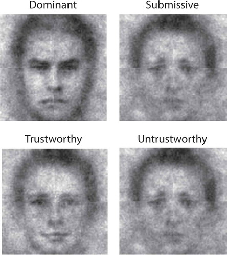
Compared to other implementations, such as photo averaging (reviewed in Sutherland, Oldmeadow, & Young, 2016) or those using computer-generated faces (reviewed in Jack & Schyns, 2017; Todorov et al., 2011), the noise-based implementation places the least constraints on the stimulus set. This allows the most freedom for features to appear in the CI that researchers did not deem relevant a priori. For instance, in a reverse correlation study where mental templates of “dominance” and “submissiveness” were investigated (Dotsch & Todorov, 2012), the CI of the dominant face showed strong contrast around the contours of the face, whereas the submissive face practically blended in with the background (see Figure 2). This feature would have probably been missed when using photos or computer-generated faces as stimulus material, although it reflects an important aspect of our subjective experience of dominant and submissive faces. Moreover, the noise-based implementation is very accessible to researchers, because the necessary software is freely available as a package in R: One needs only R (R Core Team, 2016), the rcicr package (Dotsch, 2017), and minimal coding skills.

Figure 2. CIs for dominance, submissiveness, and (un)trustworthiness (adopted with permission from Dotsch & Todorov, 2012).

The present review is a primer in noise-based reverse correlation. In the first section, we describe methodological details and provide a tutorial on the rcicr R package to create stimulus material and analyse reverse correlation data. In the second section, we highlight major achievements of the technique in social psychological research. In the discussion, we elaborate on future directions and limitations of the technique. In addition, we put forward a novel account to interpret CIs: as visual proxies of internal representations that determine how social stimuli are perceived.

Methodological details

A reverse correlation paradigm consists of four steps: (1) constructing stimulus material with random variations, (2) acquiring data by asking participants to select the images that are congruent with their mental representation, (3) computing CIs based on the responses of the participants and (4) evaluating the CIs. Here we detail these steps for the noise-based reverse correlation approach. A tutorial on how each step can be achieved using the rcicr package (Dotsch, 2017) in R is provided in the appendix.

Stimulus material

As described above, reverse correlation employs randomly varying stimuli. The implementation we discuss here uses random visual noise to create stimulus variations on some constant base image. Two main considerations at this point are which base image and what type of noise to use.

For faces, typical base images are average faces from databases (Langner et al., 2010; Lundqvist & Litton, 1998). The base face should be tailored to the particular research question and could, for example, be male, female, gender neutral or have a particular emotional expression. Importantly, the base face should match the power spectrum of the added noise as best as possible. This can be accomplished by smoothing the base image (e.g., by using a low-pass filter or Gaussian blur), which can be done with most image editing programmes. The advantage of using an averaged face as base image is that the contours of the face are often blurred while the other features of the face (eyes, mouth, nose, etc.) are in focus, making it ideal for optimal blending with the superimposed noise. Other considerations are the resolution of the base images (the more detail you want, the more trials you will need) and making the face area span as large a part of the image as possible. For sine-wave-based noise (see below), the image needs to be a perfect square and the height (and width) in pixels needs to be a power of 2. Using an inappropriate base image may lead to inadequate sampling of the information space: A base face with a closed mouth will make it hard (but not necessarily impossible) to sample the information used by social judgements requiring an open mouth.

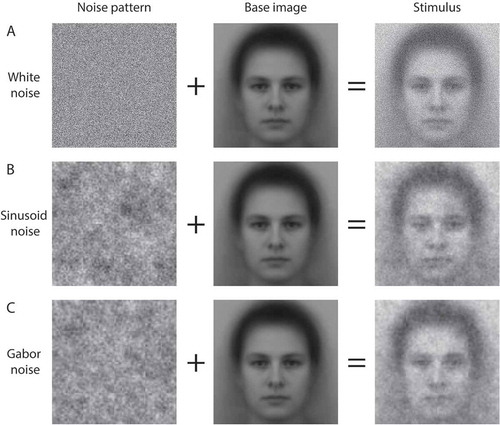
The second consideration is to choose the type of noise to create random variations on the base image. Three types of noise have been used in the literature: White noise (values are drawn from a uniform distribution), sine-wave noise and Gabor noise (Figure 3). In white noise, each pixel can take a completely random value without any constraints. The other two types of noise implement constraints that narrow the possible configurations that a noise pattern in a stimulus can have. The rationale for the constraints is that they allow the researcher to more efficiently sample relevant parts of the stimulus space (e.g., stimuli that constitute meaningful variations of faces).

Figure 3. Stimuli for noise-based reverse correlation (right column) consist of a noise pattern (left column) superimposed on a base image (middle column). The top (a), middle (b) and bottom (c) rows represent white-, sinusoid- and Gabor-noise, respectively.

In a pioneering study, Gosselin and Schyns (2003) studied the mental templates of the letter “S” using no constraints at all: Using white noise and no base image (Gosselin & Schyns, 2003). Participants were asked whether they recognised a letter “S” in stimuli that consisted of 50 × 50 pixel image of white noise. By averaging the noise patterns in the subset of trials where participants indicated that they saw the letter “S” in the stimulus, a CI was obtained which showed the letter S. The number of trials required for this task was vast: 20,000 trials. Note that the mental template of a letter is visually several orders of magnitude less complex than social stimuli. Without the constraint of a base image, the stimulus space is too large and would therefore require too many trials for typical social psychological research.

To constrain the stimulus space, subsequent studies have included a base image (a face) underneath the white noise (Figure 3(a)). Using this approach, Jack, Caldara, and Schyns (2012) visualised mental representations of emotions in Western Caucasian and East Asian participants (Jack et al., 2012). The CIs showed clear differences between the two groups. However, the number of trials in this study was still high (12,000 per participant).

To further reduce the stimulus space, a different type of noise was developed, based on superimposed sine-wave patches (Figure 3(b)), which depend on fewer parameters and match the frequency spectrum of faces (Mangini & Biederman, 2004). Detailed descriptions of how these noise patterns are constructed are provided elsewhere (Dotsch & Todorov, 2012; Mangini & Biederman, 2004). Briefly, the noise pattern is the average of five layers of sine-wave patches (2D gratings going from grey to bright to dark to grey again in a single cycle), that differ per layer in the number of cycles of the sine-wave patch (2, 4, 8, 16 or 32 cycles per patch). Each layer consists of patches that are themselves averages of 12 sine-wave patches (differing in six orientations and two phases). As such, the noise pattern is specified by 4092 parameters,¹ each specifying the contrast (amplitude) of a sine-wave patch. Hence, this type of noise allows one to efficiently sample portions of the stimulus space that vary in dimensions relevant for faces, but at the same time makes it impossible to represent visual information that cannot be encoded by sine-wave noise. Most reverse correlation studies in social psychology currently use sine-wave patches (see the following section for examples).

Recently, a third type of noise was introduced, based on Gabor patches (Figure 3(c)). The procedure to generate the noise is identical to that of sine-wave noise, but uses Gabor patches instead of sine-wave patches and is specified by 16,380 parameters² (van Rijsbergen, Jaworska, Rousselet, & Schyns, 2014). This approach yielded vivid CIs using 3240 trials per participant, with the advantage that the square artefacts visible at the border of sine-wave patches are absent. Whether Gabor noise outperforms sine-wave noise, or vice versa, has not been empirically addressed.

Once a researcher has decided on the base image and the type of noise, generating the stimuli in the rcicr package is straightforward. The required R code is provided in the Appendix (steps 1 and 2).

Data acquisition

There are various ways to set up a reverse correlation task. Specific considerations are the number of stimuli that are simultaneously presented on the screen, the number of response options, and the number of trials. Two prevalent implementations are two-image forced choice (2IFC) and four-alternative forced choice (4AFC) paradigms (Figure 1(b)). In a 2IFC task, each trial consists of two images presented side by side where participants select the image that best reflects their mental representation. The noise pattern in the image on one side of the screen is often the mathematical inverse of the noise patterns of the image on the other side of the screen.

In a 4AFC task, one image is presented per trial and participants rate the image on a 4-point scale on one (or more) dimension(s) of interest. Initially, the 4AFC task was used to rate images on a bipolar dimension (e.g., “probably male”, “possibly male”, “possibly female”, “probably male”) but the approach can equally well be used to provide weighted responses within a unipolar dimension (e.g., masculinity on a scale from 1–4). In 4AFC tasks, only the noise patterns that are categorised in one of the “probably” responses are taken into account to compute a CI. Noise patterns classified as “possibly” are usually ignored.

Formally, the 2IFC and 4AFC implementations have never been compared. The reason the 2IFC variant was originally introduced by Dotsch et al. (2008) is that in cases where the base image does not come close to the mental representation of interest (like visualising a Moroccan and Chinese face from a Scandinavian base image, as in Dotsch et al., 2008), it is very likely that none of the random stimuli will look anything like that mental representation. The result is that none of the stimuli would be classified in the “probably” category in a 4AFC task and no CI can be computed. A 2IFC task on the other hand forces each trial to be maximally diagnostic of the mental representation of interest and capitalises on the idea that after averaging, stimuli that contain no diagnostic information will compensate each other due to their randomness. The advantage of the 4AFC task is that it allows participants to include certainty judgements in their responses, which can be incorporated when calculating the CIs, as described below.

Computing CIs

The rationale for computing CIs is to visualise the parameter estimates that participants deem relevant for the classification of the stimuli. We first explain how CIs are computed for individual participants from data acquired with 2IFC tasks, and then expand to 4AFC tasks and group-level CIs.

The computation of a CI from 2IFC data of a single participant starts with averaging the selected noise patterns (Figure 1(c)). The average noise pattern is then superimposed on the base image. However, the numerical values of the average noise patterns are typically very small (due to averaging noise patterns that contain little signal and mostly random values), sometimes orders of magnitudes smaller than the range of the pixel intensities of the base image. Therefore, before overlaying the average noise pattern on the base image, the average noise pattern is scaled such that the minimum and maximum pixel intensities in the resulting CI match those of the base image.

When CIs are computed for several participants, there are two ways in which this scaling can be applied. Either we scale and maximise each CI independently or we apply a dependent scaling. The latter entails identifying the individual CI with the largest range of pixel intensities, maximising the pixel intensities for that CI by the largest scaling factor needed to match the range of the base image and then scaling the remaining CIs by that same scaling factor. The two approaches (independent versus dependent scaling) yield differences for individuals who have relatively little signal in their responses. Independent scaling will amplify the small signal present, which is accompanied by amplification of noise. Dependent scaling will lead to relatively little amplification of signal and noise for those same participants, resulting in CIs that closely resemble the original base image. Which scaling method is preferable depends on the needs of a researcher. If the researcher wants to take the strength of the signal in the CI into account, they need to use dependent scaling. Otherwise, independent scaling makes as much signal as possible visible in the CIs, at the cost of amplified noise. Both scaling options are implemented in rcicr, as demonstrated below.

Computation of CIs from 4AFC data follows the same logic, but allows the four response options to be weighted differently (Figure 1(c)). In their seminal work, Mangini and Biederman (2004) averaged the noise patterns that were classified at one (or the other) end of the response scale, although it has been shown that using appropriate weights for the different response categories can result in a higher signal-to-noise ratio (Murray, Bennett, & Sekuler, 2002). Apart from this difference, the manner in which CIs are computed for 4AFC data is identical to that of 2IFC data, with the same considerations regarding scaling.

Depending on the research question, one may be interested in CIs of groups of participants (e.g., those in one particular cell of an experimental design), rather than those of individual participants. To compute a group average CI, the unscaled noise patterns that constitute the individual-level CIs are averaged across participants in a group or condition and scaled. Importantly, computing a group-level CI in this way assumes that there is homogeneity in the mental representation of interest across subjects, which may not always be true.

The R code to generate a CI is provided in the Appendix (step 3).

Evaluating CIs

Once CIs are computed, the final step is to evaluate the CIs. Depending on the research question, this can either be done on the level of CIs of individual participants or on group aggregate CIs. A common approach to evaluate CIs is to have an independent sample of participants rate the CIs on some judgement of interest. These judgements can be used for confirmatory hypothesis testing, but only when the set of judgements have been decided on prior to seeing the CIs and when there is high inter-rater reliability. The researcher should bear in mind that a large sample of independent raters will make even the smallest differences between CIs appear significant. This is especially dangerous when independent scaling is used to compute the CIs, amplifying noise as well as signal, yielding significant differences between CIs that may very well be just noise.

An alternative approach is to objectively quantify the amount of information of a certain dimension present in a CI. This can be done by independently obtaining CIs of the dimensions the CIs are to be rated on. For example, if we are interested in the amount of trustworthiness in the CIs of male faces, we can independently collect data to compute the CI of “trustworthiness” using a standard reverse correlation task, with the same base image as used in the male reverse correlation task. We can now objectively assess the amount of trustworthiness in the male face, by correlating the male CI with the trustworthiness CI (e.g., Imhoff & Dotsch, 2013).

There are also statistical approaches that are agnostic about the specific information researchers expect to be present in CIs. One is to use pixel tests to find the pixels that significantly predict the judgement. The results can, for instance, be visualised using a z-map where each pixel represents z-scores rather than brightness, so areas of the face diagnostic for the judgement can be identified visually (e.g., Dotsch & Todorov, 2012; Jack et al., 2012; van Rijsbergen et al., 2014). The R code for computing z-maps is provided in the Appendix (step 4).

Another approach is the recently developed informational value (infoVal) statistic that quantifies the probability that an observed CI deviates from CIs generated by a purely random process. The infoVal statistic can be interpreted as a z-score. CIs without informational value (infoVal < 1.96) contain no detectable signal and should be discarded. Computation of infoVal scores of CIs is implemented in that latest version of the “rcicr” package (version 0.4.0, Dotsch, 2017). The R code to compute informational value is provided in the Appendix (step 5).

Achievements of reverse correlation

In social psychology, reverse correlation has been primarily used to identify diagnostic features that are relevant for social perception and to visualise top-down biases in social perception.

Diagnostic features

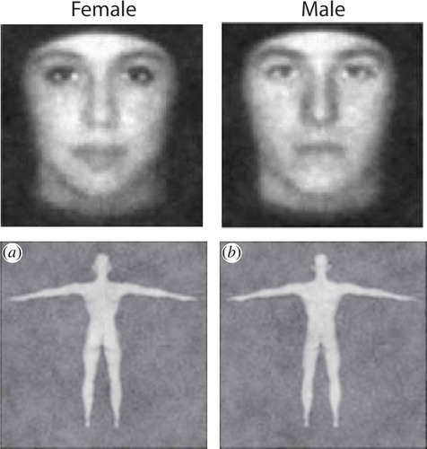
Reverse correlation’s original strength was in visualising the diagnostic features that are predictive of specific social judgements: Which facial features make someone look more male or female, more Chinese or more Moroccan, more trustworthy or more dominant? The question of which features are diagnostic can and has been posed for many social judgements, such as race, gender, age, internal states, group membership and personality. Below we review each briefly. Researchers have used reverse correlation tasks to identify features diagnostic for Black and White faces (Fiset, Wagar, Tanaka, Gosselin, & Bub, 2007; Krosch & Amodio, 2014), Moroccan faces (Dotsch et al., 2008, 2011), Chinese faces (Dotsch et al., 2008), European and Australian (Imhoff, Dotsch, Bianchi, Banse, & Wigboldus, 2011), as depicted in Figure 4. Various studies have focused on visualising the gender of faces (see Figure 5; Mangini & Biederman, 2004; Nestor & Tarr, 2008; Dotsch et al., 2011) and of bodies (Johnson, Iida, & Tassinary, 2012; Lick, Carpinella, & Preciado, 2013). To our knowledge, there is only one study that visualised age (van Rijsbergen et al., 2014). Internal states communicated through facial expressions, such as emotions, have lent themselves well to the reverse correlation technique, as they require only slight alterations of an emotionally neutral base face. Much early reverse correlation work addressed emotional expressions, visualising happy/unhappy expressions (Mangini & Biederman, 2004) or the secret to Mona Lisa’s smiling eyes (Kontsevich & Tyler, 2004). Jack, Caldara, and Schyns (2012) used reverse correlation to identify the facial information diagnostic for the six basic expressions of emotions as a function of perceiver culture (Jack et al., 2012). Going beyond emotions, researchers have employed reverse correlation to visualise facial expression of other internal states, like sexual interest (Lick, Cortland, & Johnson, 2016).

Figure 4. CIs of Black, Moroccan, Chinese, Australian and European faces (adopted from Dotsch et al., 2008, 2011; Imhoff et al., 2011; Krosch & Amodio, 2014), figures adopted with permission.

Figure 5. CIs of male (left column) and female (right column) faces and bodies (top row from Mangini & Biederman, 2004; bottom row from Johnson et al., 2012).

Most of the judgements discussed so far (race, gender, age, emotions portrayed by facial expressions) are in many cases easily and accurately discerned from faces. However, there is a subset of social judgements for which it is less clear that people can depend on visual information, namely judgements of visually (or perceptually) ambiguous groups (Tskhay & Rule, 2012). For instance, it is hard to accurately infer religion, sexual orientation, political affiliation or profession from the face alone. Although people might not be very accurate in determining people’s membership of such groups (Todorov et al., 2015), there may be a shared visual basis on which people rely to make these inferences. If so, reverse correlation should be able to identify it. Researchers have used reverse correlation to visualise diagnostic features for various professions (Hehman, Flake, & Freeman, 2015; Imhoff, Woelki, Hanke, & Dotsch, 2013), such as athletes, bankers, business men, doctors, drug dealers, financial advisors, nursery teachers, nurses, power-lifters and rappers, as well as sexual orientation (Dotsch et al., 2011; Hinzman & Maddox, 2017; Tskhay & Rule, 2015), political orientation (liberal vs. conservative; Tskhay & Rule, 2015) and various castes and religions in India (Dunham, Srinivasan, Dotsch, & Barner, 2014). Finally, Brown-Iannuzzi, Dotsch, Cooley and Payne (2017) visualised faces of welfare recipients (Brown-Iannuzzi, Dotsch, Cooley, & Payne, 2017).

A final example of diagnostic features is that reverse correlation has been used to visualise the facial features diagnostic of personality trait judgements. Dotsch and Todorov (2012) visualised trustworthiness and dominance, the two primary dimensions of face evaluation (Dotsch & Todorov, 2012). Trustworthy faces wore a subtle smile and had slightly more feminine features, whereas untrustworthy faces wore subtle angry expressions and slightly more masculine features (Figure 2). Dominance was very much related to facial masculinity. Similar efforts within this domain are the visualisation of stereotype content dimensions of warmth and competence (Imhoff et al., 2013), criminality (Dotsch et al., 2011), attractiveness (Said & Todorov, 2011), trustworthiness and dominance (Hehman et al., 2015), dominance and physical strength (Toscano, Schubert, Dotsch, Falvello, & Todorov, 2016), trustworthiness as a function of age (Éthier-Majcher, Joubert, & Gosselin, 2013) and sexual promiscuity (Lick et al., 2016).

Top-down biases

The second major use of the reverse correlation technique has been to discover top-down biases in social perception (i.e., the distortion of a mental representation due to pre-existing knowledge or motivation). Although this issue has been pursued in fewer studies, we expect to see more studies in social psychology employing reverse correlation for this purpose in the future, given the field’s traditional interest in bias.

To our knowledge, the first work to demonstrate any bias using reverse correlation was research on visual stereotypes. In two studies, Dotsch et al. (2008) showed that Dutch participants’ CIs of Moroccan faces were biased in line with their implicit evaluation of Moroccans (Figure 6; Dotsch et al., 2008). The more participants negatively evaluated Moroccans, the more criminal and less trustworthy their Moroccan CIs appeared. These results demonstrate that evaluative associations may bias people’s decisions in reverse correlation tasks. A similar bias has also been demonstrated for political candidates: Participants who supported Mitt Romney, and presumably had positive associations with him, generated CIs of Romney that appeared more positive (trustworthy) than those generated by participants who did not support him (Young, Ratner, & Fazio, 2014). Similar top-down biases have been observed for stereotype content dimensions: Visualisations of faces of male nursery teachers and managers yielded faces that were judged relatively warm-incompetent and cold-competent, respectively (Imhoff et al., 2013), as would be predicted by the stereotype content model (Fiske, Cuddy, Glick, & Xu, 2002).

Figure 6. CIs of Moroccan faces for subgroups of participants with different levels of prejudice against Moroccans (adopted with permission from Dotsch et al., 2008).

Some biases in social perception might not even require existing associations with the visualised person’s group. Ratner, Dotsch, Wigboldus, Van Knippenberg, and Amodio (2014) showed that whether a person belongs to the ingroup or an outgroup affects participants’ CI of that person (Ratner et al., 2014). Specifically, participants were first subjected to a minimal group manipulation using a dot estimation paradigm. In this task, participants were asked to estimate the number of dots appearing on the screen several times, after which they received false feedback that they were either an “over-estimator” or “under-estimator”. The feedback was in fact randomised and manipulated between subjects. Over-estimators and under-estimators then completed a reverse correlation task in which they were asked to select the face that looked the most like either an over-estimator or an under-estimator. Of interest were the ingroup CI (based on the data of over-estimators selecting over-estimators and under-estimators selecting under-estimators) and the outgroup CI (based on over-estimators selecting under-estimators and under-estimators selecting over-estimators), as depicted in Figure 7. Generally, the ingroup CI was judged more positively than the outgroup CI by independent raters. This work was extended by Paulus, Rohr, Dotsch and Wentura (2016), who visualised the interpretation of an ingroup vs. outgroup smile after assignment to minimal groups (Paulus et al., 2016). The CIs showed that smiles of ingroup members signal more benevolence than those of outgroup members.

Figure 7. CIs of ingroup and outgroup members (adopted with permission from Ratner et al., 2014).

Another example of bias visualised with reverse correlation is projection, in which participants use information about smaller more concrete social units (e.g., one’s own country in the case of ingroup-projection, or the self in the case of self-projection) in order to understand more abstract superordinate social units (e.g., inhabitants of continents). Both ingroup-projection (Imhoff et al., 2011) and self-projection (Imhoff & Dotsch, 2013) have been investigated by asking European participants to complete a reverse correlation task to visualise a European face. In Imhoff et al. (2011), there were two participant samples: German and Portuguese. The visualised European CI looked more German than Portuguese for German participants, and vice versa for Portuguese participants (Figure 4). When in a second study other German and Portuguese participants were instructed to visualise the unrelated superordinate group of Australians as control, no difference between the samples was observed in the CIs.

Because German participants tend to look more like Germans and Portuguese participants tend to look more like Portuguese people, the resulting European CI could have been biased toward the typical appearance for the respective countries through self-projection, ingroup-projection or both. To tease apart the influence of representations of self and representations of the ingroup in this projective bias, Imhoff and Dotsch (2013) asked German participants to complete three reverse correlation tasks yielding three CIs: Of self, German and European. They then computed the pixelwise correlation between each pair of CIs, as an index of similarity. Their analyses indicated that both the self and the German CIs independently explained variance in the European CIs, which can be interpreted as evidence that both self-projection and ingroup projection independently play a role when people visualise their superordinate group. Although our earlier discussion of associative and intergroup biases may have painted a picture of reverse correlation as a tool that can only tap into evaluative biases, the work on visual projection demonstrates that reverse correlation can also tap into non-evaluative biases.

Reverse correlation can also be used to investigate memory biases. Karremans, Dotsch and Corneille (2011) investigated whether being in a committed romantic relationship versus being single affects memory of the face of potential alternative partners (Karremans et al., 2011). Female participants who were in a relationship or single were first asked to memorise the face of a male. Subsequently, they completed a reverse correlation task with the instruction to select on each trial out of two noisy faces the one that looked the most like the face they had memorised. Note that the task never mentioned attractiveness, potential mates or relationships. CIs of the memorised face looked more attractive to single participants than to participants in a relationship. Female participants in a committed relationship either did not use the attractiveness dimension to encode the male face or the information was lost at retrieval. The authors speculated that this distortion may function as a relationship maintaining device, causing those who are in a committed relationship to be less motivated to approach alternative attractive mates.

General discussion

Reverse correlation has only recently been adopted in the field of social psychology, but even in these early stages the technique has proven to be an invaluable tool in the investigation of social perception (e.g., in perception of race, gender, personality traits, and internal states such as emotions). In the coming years, we expect the reverse correlation technique to become even more popular, because there are numerous potential applications of the reverse correlation approach. We elaborate on this topic in the first part of the discussion. We then briefly discuss a second reason for the increasing popularity, that is, that it is becoming increasingly easy to use reverse correlation paradigms. Third, we turn to a discussion of limitations and pitfalls. For the technique to reach its full potential, it is important to be aware of these limitations and to discuss how to deal with them. A key conceptual limitation of the technique is that it is unclear what can and cannot be inferred from CIs. In the final part of the discussion, we advance a novel perspective on how CIs can be interpreted.

Potential applications

The potential applications for reverse correlation experiments are numerous. One intriguing application is that it could give us a glimpse of what goes on in the mind of a person with mental disability. The approach can, for example, be used in clinical psychology to visualise how patients with mental disorders subjectively perceive the world (e.g., Langner, Becker, & Rinck, 2009; Richoz, Jack, Garrod, Schyns, & Caldara, 2015). We are currently running pilots to visualise aberrant mental representations in schizophrenia patients, with promising results. Identifying aberrant mental representations may provide insights into the nature of mental disorders; the images may convey aspects of the subjective experiences of patients that would otherwise be difficult to communicate. Because reverse correlation can also be applied to body images, reverse correlation can also be applied to visualise ideal and actual body images in patients suffering from Anorexia Nervosa. Pilot data from our lab suggest that reverse correlation is better able to capture features of body image than traditional measures of body image. Another potential application is in the domain of self-image where reverse correlation could be used to visualise how we (implicitly) see ourselves. Such images could serve as a diagnostic tool and could even be used in a therapeutic setting; being confronted with one’s CI of the self might result in a better understanding of oneself or one’s condition.

Ease of use

Another reason why we expect reverse correlation to become more popular in the coming years is that it is becoming increasingly easy to set up and use reverse correlation paradigms. Since 2015, the freely available open source R-package (Dotsch, 2017) makes the generation of stimuli and the computation of CIs very user friendly. As demonstrated in the Appendix, any researcher with a small amount of R knowledge should be able to compute stimuli and analyse reverse correlation data using just a few lines of code. This R-package is frequently updated with new features. Updates in the near future include functions to compute z-maps for diagnostic regions in CIs and metrics to assess data quality. The rcicr package has an active community of users and contributors, which allows users (i.e., researchers) to indicate desired features (at http://github.com/rdotsch/rcicr) to be included in later versions of the package. This makes the package versatile and able to address various outstanding research questions.

Limitations

While the findings summarised in the previous sections highlight the strengths and potential of the reverse correlation approach, it is also important to acknowledge the limitations and pitfalls of the technique. First of all, there are technical limitations that make reverse correlation less suited to address particular research questions. Second, there are no guidelines on good practice to design reverse correlation experiments or analyse reverse correlation data. Third, there is no consensus on how CIs are best interpreted.

While reverse correlation aims to visualise the content of mental representations, it can, by definition, only provide an approximation of the true mental representations. The end-product of any reverse correlation experiment (the CI) is a combination of the true mental image, the stimulus set and the performance of the participant. Even disregarding the latter, the extent to which a CI reflects true mental images is limited by the characteristics of the stimulus set. This also means that when the true mental image deviates strongly from the stimulus set, it will not be reflected accurately in the CI. For this reason, reverse correlation using noise-based stimulus material has not been very successful in the visualisation of specific person identities. Only when the base image resembles a particular individual, accurate CIs are obtained (Mangini & Biederman, 2004). Reverse correlation approaches that use computer-generated faces (instead of variants of one and the same base face) may fare better in the visualisation of person identities. In a recent study it was shown that individual faces were successfully reconstructed from memory using a reverse correlation approach that uses 3D computer-generated faces as stimulus material (Zhan, Garrod, Van Rijsbergen, & Schyns, 2017). By the same token, CIs from the noise-based reverse correlation approach are seldom as crisp as actual photos or computer-generated faces – they always contain residual noise. Moreover, the CIs are in greyscale. Adding colour to the images is technically possible (Nestor & Tarr, 2008), but the number of stimuli needed to adequately sample the stimulus space grows with each added colour dimension, making this approach less feasible.

Apart from the technical limitations, the current use of noise-based reverse correlation in social psychology is hampered by the lack of methodological work addressing validity, reliability, and guidelines for best practice. As a consequence, it is unclear how many trials and/or participants are necessary to derive robust CIs. The lack of formal criteria to make such informed decisions often leads researchers to adopt the task parameters used in previous studies, but the required task parameters may differ extensively for different mental constructs. To make informed decisions about these task parameters, one needs an objective metric to assess whether CIs contain signal and how the amount of signal depends on the number of trials in the experiment. We have recently developed such a metric, infoVal, which assessed the amount of signal relative to reverse correlation data with random responses. The metric is implemented in the latest version of the “rcicr” package (version 0.4.0) and can be used to inform the number of trials and participants in future reverse correlation experiments.

A third limitation deals with the interpretation of the CI. One of the strengths of reverse correlation is that it provides output in a visual format. These images may capture features that would otherwise be difficult to be put in words. However, this also presents a challenge, because how these images are best interpreted is not a trivial issue. In the previous section, we have seen that in social psychology results from reverse correlation studies are interpreted as either visualising top-down biases or diagnostic features. This implicit dichotomy in the interpretation of CIs is unsatisfactory and is presumably the result of different lines of research that use reverse correlation to answer different kinds of research questions. To overcome this dichotomy, we propose a more general account how CIs can be best understood.

A neurally inspired perspective on the interpretation of CIs

We propose that CIs reflect internal representations that determine how social stimuli are perceived. This notion builds on recent advances in cognitive and computational neuroscience that formalise how perception is instantiated in the brain, formally described in the theoretical framework of “predictive coding” (Clark, 2013; Friston, 2005; Summerfield & De Lange, 2014).³ The premise of this framework is that perception is all about making inferences; sensory inputs are processed and interpreted by inferring their likely causes. This notion can be traced back to seminal work by Helmholtz (1878). In the framework of predictive coding, these ideas are formalised as the interplay of (bottom-up) sensory inputs and (top-down) inferences, described in computational models with plausible neural substrates (Bastos et al., 2012; Spratling, 2017). In particular, these models describe how top-down predictions or inferences are matched to incoming sensory inputs across different levels of the cortical hierarchy. Different levels of the cortical hierarchy represent different levels of abstraction at which predictions and inferences are instantiated: Lower levels implement, for example, the continuation of regular spatial patterns behind occlusions or in the blind spot of our retina (Komatsu, 2006; Shimojo, 2014), whereas higher levels implement how we mentally represent others and their expected behaviour (Koster-Hale & Saxe, 2013). When there is a mismatch between the predicted and the received sensory inputs, a prediction-error signal is fed forward up the cortical hierarchy, which in turn evokes new or updated inferences that better match the sensory inputs. The manner in which this updating takes place hinges on the relative weights (or precision) of the sensory data and the inference, respectively. When one receives highly precise sensory inputs that do not match what one expected, this may lead to large updates of the initial inference. For example, when one expects to see a dog, but visual input is more congruent with a cat, we quickly adapt our inference to the creature being a cat. On the other hand, when sensory input is noisy and we have good reasons to expect a specific object, such as our couch in our darkened living room, we may cling more strongly to our initial inference. Through the process of prediction-error minimisation, the system converges on the most likely interpretation.

Key to this framework is the notion of a generative model, which is where all predictions and inferences originate (Friston, 2010). The generative model comprises everything that we have mentally internalised: Concepts, contingencies and representations of our current bodily and mental state. It predicts anticipated sensory inputs, consistent with our current understanding of what is out there in the world and, by the same token, allows us to converge on the most likely interpretation of sensory inputs by updating our initial inferences. While most research in the domain of predictive coding is focused on the first part (how expectations shape perception, as reviewed in Summerfield & De Lange, 2014), for present purposes the second part is crucial: How inferences are updated during convergence. The updating of inferences is determined by the range of possible inferences and the estimated likelihood of those inferences, which together form the unique instantiation of the generative model of a person. The generative model can also be described as the collection of all mental representations. As such, social perception is shaped by the content of mental representations of socially relevant dimensions, where interindividual differences in social perception can be attributed to differences in those mental representations. In previous sections, we argued that CIs reflect the contents of such mental templates. We therefore propose that CIs reflect internal representations that determine how social stimuli are perceived. This suggestion is fully compatible with the notion that CIs reflect top-down biases, as discussed in previous sections. However, the current notion goes one step further: Given the profound role of top-down effects in determining the contents of perception in the framework of predictive coding, we propose that the top-down biases reflected in CIs have a causal influence on social perception.

To return to the example in the introduction, when we determine whether we can trust someone or not, we match our mental template of trustworthiness to the facial appearance of the stranger. If there is a match, we infer that the stranger can be trusted. What we perceive is determined by our mental representation, of which the CI is a visual reflection.

The proposal that CIs are visual proxies of determinants of social perception is open for empirical investigation. Although this notion has not been formally tested, several empirical observations are compatible with this proposal. For example, if CIs truly represent determinants of social perceptions, interindividual differences in CIs should reflect interindividual differences in social perception. This was observed in a study in which participants who differed in their prejudice against Moroccans yielded qualitatively different CIs of a typical Moroccan face (Dotsch et al., 2008). Prejudice was measured with a single-target Implicit Association Task (ST-IAT; Bluemke & Friese, 2008), where participants categorise in parallel words with positive and negative connotations (on valence) and Moroccan names, using the same response options. Prejudice was inferred from slower response times when Moroccan names were categorised with the same response option as words with positive valance. The extent to which CIs looked “criminal”, as judged by independent raters, correlated with the amount of prejudice exhibited by participants. Reconsidering these findings, we propose that the mental representation of a Moroccan face not only reflects one’s prejudice but also determines how the person (implicitly) perceives and evaluates Moroccan names.

Moreover, in a study on social categorisation, participants with a negative bias towards Moroccans (again measured with a ST-IAT) were more likely to categorise criminal-looking faces as Moroccan (Dotsch et al., 2011). Reinterpreting these findings, we suggest that the (biased) mental representation of participants determines both the performance on the ST-IAT and the bias in categorisation.

In a different study, Dotsch, Wigboldus, and Van Knippenberg (2013) used reverse correlation to visualise what people expected faces of members of novel groups to look like (Dotsch et al., 2013). In a learning phase, participants learned to associate positive (trustworthy) or negative (criminal) behaviours with an a priori meaningless Group X. The behavioural information about Group X members was provided alongside noisy images of exemplar faces, identical across experimental conditions. After the learning phase, participants performed a reverse correlation task on the expected facial appearance of a typical Group X member. The resulting CIs were in line with the experimental manipulation: The CIs of participants who previously learned that Group X members were more trustworthy were rated as more trustworthy and less criminal, and vice versa. In addition, the ratings of the CIs correlated with implicit and explicit measures of bias toward outgroup members. Revisiting these results, we suggest that the mental representation of Group X members determined the performance on the tasks that measured implicit and explicit bias toward Group X members and that the CI is a visual proxy of that mental representation.

The suggestion that CIs are visual proxies of determinants of social perception is novel and needs further empirical investigation to establish how fruitful and solid this notion is. A next step would be to formalise these suggestions in a Bayesian computational model, in line with formalisations in the predictive coding framework. Such a model would provide precise empirical predictions about interindividual differences in social perception and can be used to validate or falsify the suggestion that CIs truly reflect determinants of social perception.

Conclusion

Although the noise-based reverse correlation technique has been adopted by social psychologists only in the last decade, it has proven to be an invaluable tool to access mental representations relevant for categorisation of race, gender, personality traits and internal states such as emotions. Moreover, the technique can be used to address many interesting and outstanding questions, for example, investigating (aberrant) mental representations in people with mental disorders. However, before the technique can be successfully deployed in these domains, several methodological issues need to be resolved. The most important issue is the development of an overarching theoretical framework for interpreting CIs. Here we have sketched the outline of such a framework, advancing the notion that CIs are best understood as visual read-outs of the determinants of (social) perception.

Acknowledgements

This work was supported by the Psychology department of Utrecht University, The Netherlands; the Neuroscience & Cognition program of Utrecht University, The Netherlands; and the Netherlands Organisation for Scientific Research (NWO) under grant number 452-11-014 (personal VIDI grant: N.E.M. van Haren). We thank Peter Kok (Yale University, USA) and Ruud Custers (Utrecht University, The Netherlands) for insightful comments regarding the predictive coding framework.

Notes

¹ In comparison, the number of parameters for patches of white noise is equal to the number of pixels, which typically amounts to 512 × 512 = 262,144 parameters.

² Note that in this study, six layers of noise were specified, which allows for more local (high-frequency) modulations of the base image. It is this extra layer that increases the number of parameters, not the noise type per se.

³ In a recent preprint, Zhan et al. (2017) have also interpreted CIs in the context of the predictive coding framework. Their emphasis is on memories as the source of predictions and how these are reflected in the mental representations of person identities. This account does not discuss the possibility of causal influences of CIs on social perception, which is key to the suggestion we put forward here.

⁴ Note that there are various approaches to computing the z-map, and these are all detailed in the documentation of rcicr.

Appendix

Tutorial for noise-based reverse correlation using the rcicr R package

Step 1: Installing the rcicr package

The development version of rcicr (version 0.4.0) can be installed and loaded as follows from within R.

install.packages(“devtools”)

devtools::install_github(“rdotsch/rcicr”, ref = “development”)

library(rcicr)

Note that rcicr is under continuous development and that the syntax below may change in the future. The up-to-date syntax is always stated in the accompanying documentation, which you can access through R’s help system after installing the package.

Step 2: Generating stimuli

Assuming the base image file is called “base.jpg” and resides in your current working directory, you can generate stimuli for 300 trials as follows:

generateStimuli2IFC(list(base =“base.jpg”), n_trials = 300)

This line of code will create stimuli as .png images in a folder called “stimuli” with a default resolution of 512 × 512 pixels (which the base image file should match). These files can subsequently be used with your program of choice for data acquisition. The code will also generate a .Rdata file that stores all the parameter values corresponding to each stimulus. This file is used later in the analysis. By default, this line of code will generate stimuli with sine-wave-based noise. The line above can easily be adapted to generate stimuli with Gabor noise or to set various other options for the noise, although we recommend using default settings. To read the documentation for all the options that can be set, use the following line:

?generateStimuli2IFC

The stimulus files generated here can be used for both a 2IFC and a 4IFC task. The code generates two stimulus files per trial, one with “ori” in the filename, indicating that this is the main stimulus with the original random noise pattern for that trial superimposed, which is the one you should present in a 4IFC task. The stimulus file with “inv” in the filename is the stimulus with the mathematical opposite of that same random noise pattern superimposed (“inv” stands for inverted: Dark noise pixels become bright and vice versa). In a 2IFC task you would present both the original and the inverted stimuli side-by-side on a single trial.

Step 3: Computing classification images

The R code to generate the CI is:

# Path to rdata-file holding all stimulus parameters, created when generating stimuli

rdata <- “stimuli/parameters.Rdata”

ci <- generateCI(S$stim, S$response, “base”, rdata)

Here, “base” refers to the name of the base image, as specified in the .Rdata file. By default, independent scaling will be used. Dependent scaling only makes sense when there are multiple participants in the data set. Let G be the same data frame as S, but now with data from multiple participants and an additional column stating subject number called “subnum”. With the development version you can now generate all participant images with dependent scaling with the following code (previous versions used the batchGenerateCI2IFC function):

cis <- generateCI(G$stim, G$response, “base”, rdata,

participants=G$subnum, individual_scaling = “dependent”,

save_individual_cis = TRUE)

The code will generate the individual CIs with dependent scaling as well as the group-level CI with independent scaling as default.

Step 4: Computing z-maps

Z-maps are computed in R with the following code for an individual participant’s CI⁴:

ci <- generateCI(S$stim, S$response, “base”, rdata, zmap = TRUE, zmapmethod = “t.test”)

Step 5: Computing informational value

Informational value of CIs can be computed as follows:

infoVal <- computeInfoVal2IFC(ci, rdata)

Here, “ci” and “rdata” are variables that have been declared in the previous lines of code (see above).

References

- Ahumada, A., & Lovell, J. (1971). Stimulus features in signal detection. The Journal of the Acoustical Society of America, 49(6B), 1751–1756. doi:10.1121/1.1912577
- Bastos, A. M., Usrey, W. M., Adams, R. A., Mangun, G. R., Fries, P., & Friston, K. J. (2012). Canonical microcircuits for predictive coding. Neuron, 76(4), 695–711. doi:10.1016/j.neuron.2012.10.038
- Beard, B. L., & Ahumada, A. J. (1998). A technique to extract relevant image features for visual tasks. Proceedings of SPIE, 3299, 79. doi:10.1117/12.320099
- Bluemke, M., & Friese, M. (2008). Reliability and validity of the Single-Target IAT (ST-IAT): Assessing automatic affect towards multiple attitude objects. European Journal of Social Psychology, 38, 977–997. doi:10.1002/ejsp.487
- Brown-Iannuzzi, J. L., Dotsch, R., Cooley, E., & Payne, B. K. (2017). The relationship between mental representations of welfare recipients and attitudes toward welfare. Psychological Science, 28(1), 92–103. doi:10.1177/0956797616674999
- Clark, A. (2013). Whatever next? Predictive brains, situated agents, and the future of cognitive science. Behavioral and Brain Sciences, 36, 181–253. doi:10.1017/S0140525X12000477
- Coenders, M., Lubbers, M., Scheepers, P., & Verkuyten, M. (2008). More than two decades of changing ethnic attitudes in the Netherlands. Journal of Social Issues, 64(2), 269–285. doi:10.1111/j.1540-4560.2008.00561.x
- Dotsch, R. (2017). rcicr: Reverse correlation image classification toolbox. R package version 0.4.0. https://CRAN.R-project.org/package=rcicr
- Dotsch, R., & Todorov, A. (2012). Reverse correlating social face perception. Social Psychological and Personality Science, 3(5), 562–571. doi:10.1177/1948550611430272
- Dotsch, R., Wigboldus, D. H. J., Langner, O., & Van Knippenberg, A. (2008). Ethnic out-group faces are biased in the prejudiced mind. Psychological Science, 19(10), 978–980. doi:10.1111/j.1467-9280.2008.02186.x
- Dotsch, R., Wigboldus, D. H. J., & van Knippenberg, A. (2011). Biased allocation of faces to social categories. Journal of Personality and Social Psychology, 100(6), 999–1014. doi:10.1037/a0023026
- Dotsch, R., Wigboldus, D. H. J., & Van Knippenberg, A. (2013). Behavioral information biases the expected facial appearance of members of novel groups. European Journal of Social Psychology, 43(1), 116–125. doi:10.1002/ejsp.1928
- Dunham, Y., Srinivasan, M., Dotsch, R., & Barner, D. (2014). Religion insulates ingroup evaluations: The development of intergroup attitudes in India. Developmental Science, 17(2), 311–319. doi:10.1111/desc.12105
- Eckstein, M. P., & Ahumada, A. (2002). Classification images: A tool to analyze visual strategies. Journal of Vision, 2(1), 1–2. doi:10.1167/2.1.i
- Éthier-Majcher, C., Joubert, S., & Gosselin, F. (2013). Reverse correlating trustworthy faces in young and older adults. Frontiers in Psychology, 4, 592. doi:10.3389/fpsyg.2013.00592
- Fiset, D., Wagar, B., Tanaka, J., Gosselin, F., & Bub, D. (2007). The face of race: Revealing the visual prototype of black and white faces in Caucasian subjects. Journal of Vision, 7(99), 10. doi:10.1167/7.9.10
- Fiske, S. T., Cuddy, A. J. C., Glick, P., & Xu, J. (2002). A model of (often mixed) stereotype content: Competence and warmth respectively follow from perceived status and competition. Journal of Personality and Social Psychology, 82(6), 878–902. doi:10.1037/0022-3514.82.6.878
- Freeman, J. B., & Ambady, N. (2014). The dynamic interactive model of person construal: Coordinating sensory and social processes. Dual-Process Theories of the Social Mind, 235–248. doi:10.1037/a0022327
- Friston, K. (2005). A theory of cortical responses. Philosophical Transactions of the Royal Society B: Biological Sciences, 360(1456), 815–836. doi:10.1098/rstb.2005.1622
- Friston, K. (2010). The free-energy principle: A unified brain theory? Nature Reviews Neuroscience, 11(2), 127–138. doi:10.1038/nrn2787
- Gosselin, F., & Schyns, P. G. (2003). Superstitious perceptions reveal properties of internal representations. Psychological Science, 14(5), 505–509. doi:10.1111/1467-9280.03452
- Greenwald, A. G., McGhee, D. E., Schwartz, J. L. K., & Attitudes, M. I. (1998). Measuring individual differences in implicit cognition: The implicit association test. Journal of Personality, 74(6), 1464–1480. doi:10.1037/0022-3514.74.6.1464
- Greenwald, A. G., Nosek, B. A., & Banaji, M. R. (2003). Understanding and using the Implicit Association Test: I. An improved scoring algorithm. Journal of Personality and Social Psychology, 85(2), 197–216. doi:10.1037/0022-3514.85.2.197
- Hehman, E., Flake, J. K., & Freeman, J. B. (2015). Static and dynamic facial cues differentially affect the consistency of social evaluations. Personality and Social Psychology Bulletin, 41(8), 1123–1134. doi:10.1177/0146167215591495
- Helmholtz, H. (1878). The facts of perception. In Selected writings of Hermann Helmholtz (pp. 1–17). Madison: University of Wisconsin.
- Hinzman, L., & Maddox, K. B. (2017). Conceptual and visual representations of racial categories: Distinguishing subtypes from subgroups. Journal of Experimental Social Psychology, 70(May), 95–109. doi:10.1016/j.jesp.2016.12.012
- Imhoff, R., & Dotsch, R. (2013). Do we look like me or like us? Visual projection as self- or ingroup-projection. Social Cognition, 31(6), 806–816. doi:10.1521/soco.2013.31.6.806
- Imhoff, R., Dotsch, R., Bianchi, M., Banse, R., & Wigboldus, D. H. J. (2011). Facing Europe: Visualizing spontaneous in-group projection. Psychological Science, 22(12), 1583–1590. doi:10.1177/0956797611419675
- Imhoff, R., Woelki, J., Hanke, S., & Dotsch, R. (2013). Warmth and competence in your face! Visual encoding of stereotype content. Perception Science, 4(June), 386. doi:10.3389/fpsyg.2013.00386
- Jack, R. E., Caldara, R., & Schyns, P. G. (2012). Internal representations reveal cultural diversity in expectations of facial expressions of emotion. Journal of Experimental Psychology: General, 141(1), 19–25. doi:10.1037/a0023463
- Jack, R. E., & Schyns, P. G. (2017). Toward a social psychophysics of face communication. Annual Review of Psychology, 68(1), 269–297. doi:10.1146/annurev-psych-010416-044242
- Johnson, K. L., Iida, M., & Tassinary, L. G. (2012). Person (mis)perception: Functionally biased sex categorization of bodies. Proceedings of the Royal Society B: Biological Sciences, 279(1749), 4982–4989. doi:10.1098/rspb.2012.2060
- Karremans, J. C., Dotsch, R., & Corneille, O. (2011). Romantic relationship status biases memory of faces of attractive opposite-sex others: Evidence from a reverse-correlation paradigm. Cognition, 121(3), 422–426. doi:10.1016/j.cognition.2011.07.008
- Komatsu, H. (2006). The neural mechanisms of perceptual filling-in. Nature Reviews Neuroscience, 7(3), 220–231. doi:10.1038/nrn1869
- Kontsevich, L. L., & Tyler, C. W. (2004). What makes Mona Lisa smile? Vision Research, 44(13), 1493–1498. doi:10.1016/j.visres.2003.11.027
- Koster-Hale, J., & Saxe, R. (2013). Theory of mind: A neural prediction problem. Neuron, 79(5), 836–848. doi:10.1016/j.neuron.2013.08.020
- Krosch, A. R., & Amodio, D. M. (2014). Economic scarcity alters the perception of race. Proceedings of the National Academy of Sciences, 111(25), 9079–9084. doi:10.1073/pnas.1404448111
- Langner, O., Becker, E. S., & Rinck, M. (2009). Social anxiety and anger identification: Bubbles reveal differential use of facial information with low spatial frequencies. Psychological Science, 20(6), 666–670. doi:10.1111/j.1467-9280.2009.02357.x
- Langner, O., Dotsch, R., Bijlstra, G., Wigboldus, D. H. J., Hawk, S. T., & Van Knippenberg, A. (2010). Presentation and validation of the Radboud Faces Database. Cognition & Emotion, 24(8), 1377–1388. doi:10.1080/02699930903485076
- Lick, D. J., Carpinella, C. M., & Preciado, M. A. (2013). Reverse-correlating mental representations of sex-typed bodies: The effect of number of trials on image quality. Frontiers in Psychology. doi:10.3389/fpsyg.2013.00476/abstract
- Lick, D. J., Cortland, C. I., & Johnson, K. L. (2016). The pupils are the windows to sexuality: Pupil dilation as a visual cue to others’ sexual interest. Evolution and Human Behavior, 37(2), 117–124. doi:10.1016/j.evolhumbehav.2015.09.004
- Lundqvist, D., & Litton, J. E. (1998). The averaged Karolinska directed emotional faces—AKDEF [CD ROM]. Stockholm: Karolinska Institutet.
- Mangini, M. C., & Biederman, I. (2004). Making the ineffable explicit: Estimating the information employed for face classifications. Cognitive Science, 28(2), 209–226. doi:10.1207/s15516709cog2802_4
- Murray, R. F., Bennett, P. J., & Sekuler, A. B. (2002). Optimal methods for calculating classification images: Weighted sums. Journal of Vision, 2(1), 79–104. doi:10.1167/2.1.6
- Nestor, A., & Tarr, M. J. (2008). Gender recognition of human faces using color. Psychological Science, 19(12), 1242–1246. doi:10.1111/j.1467-9280.2008.02232.x
- Paulus, A., Rohr, M., Dotsch, R., & Wentura, D. (2016). Positive feeling, negative meaning: Visualizing the mental representations of in-group and out-group smiles. PLoS ONE, 11(3), 1–18. doi:10.1371/journal.pone.0151230
- R Core Team. (2016). R: A language and environment for statistical computing. Vienna, Austria: R Foundation for Statistical Computing. Retrieved from https://www.R-project.org/
- Ratner, K. G., Dotsch, R., Wigboldus, D. H. J., Van Knippenberg, A., & Amodio, D. M. (2014). Visualizing minimal ingroup and outgroup faces: Implications for impressions, attitudes, and behavior. Journal of Personality and Social Psychology, 106(66), 897–911. doi:10.1037/a0036498
- Richoz, A.-R., Jack, R. E., Garrod, O. G. B., Schyns, P. G., & Caldara, R. (2015). Reconstructing dynamic mental models of facial expressions in prosopagnosia reveals distinct representations for identity and expression. Cortex, 65, 50–64. doi:10.1016/j.cortex.2014.11.015
- Said, C. P., & Todorov, A. (2011). A statistical model of facial attractiveness. Psychological Science, 22(9), 1183–1190. doi:10.1177/0956797611419169
- Shimojo, S. (2014). Postdiction: Its implications on visual awareness, hindsight, and sense of agency. Frontiers in Psychology, 5(MAR), 1–19. doi:10.3389/fpsyg.2014.00196
- Spratling, M. W. (2017). A review of predictive coding algorithms. Brain and Cognition, 112, 92–97. doi:10.1016/j.bandc.2015.11.003
- Summerfield, C., & De Lange, F. P. (2014). Expectation in perceptual decision making: Neural and computational mechanisms. Nature Reviews Neuroscience, (October), 1–12. doi:10.1038/nrn3838
- Sutherland, C. A. M., Oldmeadow, J. A., & Young, A. W. (2016). Integrating social and facial models of person perception: Converging and diverging dimensions. Cognition, 157, 257–267. doi:10.1016/j.cognition.2016.09.006
- Todorov, A., Dotsch, R., Wigboldus, D. H. J., & Said, C. P. (2011). Data-driven methods for modeling social perception. Social and Personality Psychology Compass, 5(10), 775–791. doi:10.1111/j.1751-9004.2011.00389.x
- Todorov, A., Olivola, C. Y., Dotsch, R., & Mende-Siedlecki, P. (2015). Social attributions from faces: Determinants, consequences, accuracy, and functional significance. Annual Review of Psychology, 66(1), 519–545. doi:10.1146/annurev-psych-113011-143831
- Toscano, H., Schubert, T. W., Dotsch, R., Falvello, V., & Todorov, A. (2016). Physical strength as a cue to dominance. Personality and Social Psychology Bulletin, 42(12), 1603–1616. doi:10.1177/0146167216666266
- Tskhay, K. O., & Rule, N. O. (2012). Accuracy in categorizing perceptually ambiguous groups: A review and meta-analysis. Personality and Social Psychology Review, 17(11), 72–86. doi:10.1177/1088868312461308
- Tskhay, K. O., & Rule, N. O. (2015). Emotions facilitate the communication of ambiguous group memberships. Emotion, 15(6), 812–826. doi:10.1037/emo0000077
- van Rijsbergen, N., Jaworska, K., Rousselet, G. A., & Schyns, P. G. (2014). With age comes representational wisdom in social signals. Current Biology, 24(23), 2792–2796. doi:10.1016/j.cub.2014.09.075
- Verkuyten, M., & Zaremba, K. (2005). Interethnic relations in a changing political context. Social Psychology Quarterly, 68(4), 375–386. doi:10.1177/019027250506800405
- Young, A. I., Ratner, K. G., & Fazio, R. H. (2014). Political attitudes bias the mental representation of a presidential candidate’s face. Psychological Science, 25(2), 503–510. doi:10.1177/0956797613510717
- Zhan, J., Garrod, O. G. B., Van Rijsbergen, N., & Schyns, P. G. (2017). Efficient information contents flow down from memory to predict the identity of faces. BioRxiv, 44(0), 1–35. doi:10.1101/125591