Uncertainties in PM_2.5 Gravimetric and Speciation Measurements and What We Can Learn from Them

ABSTRACT

The U.S. Environmental Protection Agency (EPA) and the federal land management community (National Park Service, United States Fish and Wildlife Service, United States Forest Service, and Bureau of Land Management) operate extensive particle speciation monitoring networks that are similar in design but are operated for different objectives. Compliance (mass only) monitoring is also carried out using federal reference method (FRM) criteria at approximately 1000 sites. The Chemical Speciation Network (CSN) consists of approximately 50 long-term-trend sites, with about another 250 sites that have been or are currently operated by state and local agencies. The sites are located in urban or suburban settings. The Interagency Monitoring of Protected Visual Environments (IMPROVE) monitoring network consists of about 181 sites, approximately 170 of which are in nonurban areas. Each monitoring approach has its own inherent monitoring limitations and biases. Determination of gravimetric mass has both negative and positive artifacts. Ammonium nitrate and other semivolatiles are lost during sampling, whereas, on the other hand, measured mass includes particle-bound water. Furthermore, some species may react with atmospheric gases, further increasing the positive mass artifact. Estimating aerosol species concentrations requires assumptions concerning the chemical form of various molecular compounds, such as nitrates and sulfates, and organic material and soil composition. Comparing data collected in the various monitoring networks allows for assessing uncertainties and biases associated with both negative and positive artifacts of gravimetric mass determinations, assumptions of chemical composition, and biases between different sampler technologies. All these biases are shown to have systematic seasonal characteristics. Unaccounted-for particle-bound water tends to be higher in the summer, as does nitrate volatilization. The ratio of particle organic mass divided by organic carbon mass (Roc) is higher during summer and lower during the winter seasons in both CSN and IMPROVE networks, and Roc is lower in urban than nonurban environments.

IMPLICATIONS

Particulate matter less than 2.5 microns in size (PM_2.5) National Ambient Air Quality Standards (NAAQS) are based on gravimetric analysis of particulate matter collected on a Teflon substrate, using federal reference methodologies, whereas compliance under the Regional Haze Rule (RHR) is based on atmospheric extinction, derived from measurements of individual aerosol species. Gravimetric mass can be over- or underestimated because of volatilization issues and water retention by inorganic species, whereas species-specific estimates of mass are dependent on assumptions concerning their detailed chemical composition. Over- or underestimation of aerosol species or gravimetric mass could result in violation of standards or failure to meet visibility goals established under the RHR.

INTRODUCTION

The U.S. Environmental Protection Agency (EPA) and the federal land management community (National Park Service, United States Fish and Wildlife Service, United States Forest Service, and Bureau of Land Management) are responsible for the operation of two extensive particle monitoring networks that are similar in their design but serve different objectives. The Chemical Speciation Network (CSN)1 consists of approximately 50 long-term-trend sites, with about another 250 sites that are or have been operated by state and local agencies. The sites are located in urban and suburban settings. The objectives of the CSN are to track progress of emission control programs, develop emission control strategies, and characterize annual and seasonal spatial and temporal trends. The CSN data are also used for validating regional air quality models and source apportionment modeling and for linking health effect endpoints to constituents in particulate matter less than 2.5 microns in size (PM_2.5). National Aerosol Air Quality Standards (NAAQS) compliance (mass only) monitoring is also carried out using federal reference methods (FRMs) at approximately 1000 sites.2

The Interagency Monitoring of Protected Visual Environments (IMPROVE) monitoring network consists of about 181 sites, approximately 170 of which are in nonurban areas.3 The IMPROVE monitoring program is used primarily to track long-term temporal changes in visibility in protected visual environments, consistent with the needs of the Regional Haze Rule (RHR).4 Compliance under the RHR is based on reconstructed aerosol mass and light extinction from aerosol composition. Data collected in IMPROVE are also used to identify chemical species and emission sources responsible for existing man-made visibility impairment in federal Class I areas, for identification of episodes of long-range transport (e.g., smoke, dust, sulfates, nitrates, etc., from distant sources), to serve as a regional backdrop for special studies, for regional modeling validation studies, and to support the development and implementation of PM_2.5 NAAQS by characterizing nonurban regional background levels (see Sections 169A and 169B of the Clean Air Act (42) U.S.C. §§ 7491, 7492, and implementing regulations at 40 CFR 51.308 and 51.309, containing legally binding requirements).

The PM_2.5 speciation target analytes for both monitoring networks are similar and consist of an array of ions, carbon species, and trace elements.3,5 Each series of analytes requires sample collection on an appropriate filter medium to allow chemical analysis with methods of adequate sensitivity. The methods used for analyses of these filter media include gravimetry (electro-microbalance) for mass; energy-dispersive X-ray fluorescence for trace elements; ion chromatography (IC) for anions and cations; and controlled-combustion thermal optical transmittance and reflectance (TOT/TOR) analysis for carbon.

PM_2.5 compliance monitoring is based on the gravimetric mass concentrations, whereas determining progress toward natural visibility conditions under RHR requirements is achieved through estimations of extinction, using speciated mass concentrations and measured relative humidity (RH). Each approach has its own inherent monitoring limitations. PM_2.5 mass is determined gravimetrically by pre- and post-weighing of Teflon filter media, after equilibrating at 20–23°C and 30–40% RH. Determination of gravimetric mass using this procedure has both negative and positive artifacts. Ammonium nitrate and other semivolatiles, such as some organic species, are, in part, lost during sampling, whereas, on the other hand, measured mass includes particle-bound water associated with hygroscopic species such as sulfates, nitrates, sea salt, and possibly some organic species.6 Furthermore, some species may react with atmospheric gases, which tend to contribute to a positive artifact. Conditions under which filter substrates are shipped as well as on-site storage practices can also affect retention and evolution of collected aerosol material.

The RHR specifies that measured individual species concentrations be converted to total mass concentrations and extinction. The total mass derived from measured species will be referred to as reconstructed mass. It is assumed that sulfates are fully neutralized as ammonium sulfate, nitrates are in the form of ammonium nitrate, organic carbon mass is estimated from measured organic carbon that has been estimated using TOT/TOR techniques, soil mass is estimated assuming oxide forms of measured soil elements, and sea salt is estimated from chloride measurements.3 Each of these estimates may be high or low, depending on actual molecular composition of the aerosol. Semivolatile organic compound (SVOC) species may volatilize, causing organic carbon to be underestimated, whereas the Roc factor (organic mass/organic carbon) varies as a function of carbon molecular structure.

This paper explores differences in measured organic carbon resulting from using different sampling systems and the implied difference this has on gravimetric mass. Comparison of measured gravimetric mass to reconstructed speciated mass allows for estimating the difference in measured gravimetric and reconstructed mass concentrations as compared to an estimate of true ambient PM_2.5 concentrations. Identified differences will be explored as a function of season and of urban, suburban, and remote locations. The spatial and seasonal variations in the Roc factor, nitrate volatilizations, and retained water on the Teflon filter at the time of weighing will also be explored.

SAMPLE COLLECTION SYSTEMS

Chow et al.7 provide an overview of sampling procedures and protocols for most particulate samplers that are currently being used, including the IMPROVE samplers and the five samplers that have historically been operated in the CSN. Table 1 summarizes these sampler and sampling characteristics, including the number of channels, flow rate, and filter face velocity. The five samplers are referred to as Anderson, Met One, URG, R&P 2300, and R&P 2025.

Table 1. Design specifications of the IMPROVE and CSN samplers

	IMPROVE	CSN	CSN	CSN	CSN	CSN
Sampler type	IMPROVE	Andersen RAAS	Met One SASS	URG MASS	R&P 2300	R&P 2025 sequential FRM
Number of sites (2006)	181	18	179	6	14	22
Number of channels	4	4	5	2	4	2
Flow rate	22.7 L/min	7.3 L/min	6.7 L/min	16.7 L/min	10.0 L/min	16.7 L/min
Filter face velocity	107.2 cm/sec	10.3 cm/sec	9.5 cm/sec	23.7 cm/sec	14.2 cm/sec	23.6 cm/sec
Sampling frequency	3rd day	3rd day	3rd day	3rd day	3rd day/6th day	3rd day/6th day
Quartz filter pack configuration	Q for QBQ	QF	QF	QF	QF	QF
Quartz filter type	25-mm Pall	47-mm Whatman	47-mm Whatman	47-mm Whatman	47-mm Whatman	47-mm Whatman

Interagency Monitoring of Protected Visual Environments (IMPROVE)

A full discussion of site locations and monitoring protocols is presented by Malm et al.3,8 and Hand and Malm.9 The IMPROVE data are available online at http://views.cira.colostate.edu/web/DataWizard/.

The IMPROVE sampler consists of four independent modules. Each module incorporates a separate inlet array, filter pack, and pump assembly; however, all modules are controlled by the same singular timing mechanism. It is convenient to consider a particular module, its associated filter, and the parameters measured from the filter as a channel of measurement (e.g., channel A).

Channels A, B, and C are equipped with 2.5-µm cyclones. The channel A Teflon filter is analyzed for fine mass (PM_2.5) gravimetrically; nearly all elements with atomic mass number >11 (which is Na) and <82 (which is Pb) by X-ray florescence; elemental hydrogen by proton elastic scattering analysis; and light absorption.

Channel B utilizes a sodium carbonate denuder to remove nitric acid, followed by a single Nylasorb filter as a collection substrate. The material collected from the filter is extracted ultrasonically in an aqueous solution that is subsequently analyzed by IC for the anions sulfate, nitrate, nitrite, and chloride.

Channel C utilizes tandem quartz fiber filters for the collection of fine particles and the estimation of the organic carbon artifact from organic gases collected on the secondary filter. These filters are analyzed by TOR for elemental and organic carbon.10 The reported carbon concentrations are corrected for an approximate positive artifact.11 The IMPROVE correction method uses monthly median organic carbon mass measured on backup quartz filters from six nonurban sites, and then this seasonal correction is applied across the entire IMPROVE network.12,13 This assumes that the adsorbed gaseous material mass is equal throughout the continental United States. The method also assumes that the vapors are adsorbed uniformly throughout the front and back filters (adsorption capacity is attained). Both these assumption may not always be true.13

Channel D, fitted with a PM₁₀ inlet, utilizes a Teflon filter, which is gravimetrically analyzed for mass (PM₁₀). Exposed cassettes collected in all channels are placed in sealed plastic bags and shipped for storage under ambient conditions.

The Chemical Speciation Network (CSN)

The CSN data are available online at http://www.epa.gov/ttn/airs/airsaqs/detaildata/downloadaqsdata.htm.

Substrates and analytic procedures used in the CSN are similar to IMPROVE. However, there are important differences between the networks. In the CSN, the sample collected on the Nylasorb filter is analyzed for both anions and cations, and PM₁₀ samples are not collected. In addition, the quartz filters are analyzed using TOT and a method similar to the National Institute for Occupational Safety and Health (NIOSH) 5040 protocol. The carbon concentrations are not corrected for a positive organic carbon artifact.10,14–17 Last, samples are shipped cold from the field to the laboratories for analysis. A general discussion of the handling of laboratory and field blanks can be found in Chow and Watson.14

Although the networks have these differences, comparison of collocated data shows that the PM_2.5 mass concentrations, anions, and a number of the elemental components are in general agreement between the networks. However, there are significant differences in the carbon concentrations.

Exploration of the Differences in the IMPROVE and CSN Carbon Measurements

Collection of PM_2.5 samples on quartz fiber filters, followed by thermal optical analysis for organic carbon (OC) and elemental carbon (EC) content, is subject to a number of artifacts. This includes sampling artifacts due to adsorption of volatile organic compound (VOC) gases by the quartz fiber filter, leading to positive additive artifacts,13,18 and evaporation of particles, leading to negative artifacts proportional to the SVOCs.19 In addition, filter handling procedures and thermal optical analysis protocols can cause artifacts and differences in the OC and EC concentrations.11,20 The following explores the differences between the IMPROVE and CSN carbon concentrations at collocated sites and develops relationships to reconcile these differences. Others have also explored the carbon artifacts in the IMPROVE, CSN, and other networks. Most recently, White,21 Watson et al.,13 and Chow et al.12 performed a number of analyses, including the examination of field blanks, backup quartz fiber filters, and collocated carbon data, to assess the sampling artifacts and their causes. The following is based on work by White.21 The analysis is similar to some of those by Chow et al.,12 but we develop a different physical model, use different sets of data, and estimate monthly artifacts as opposed to seasonal and annual artifacts.

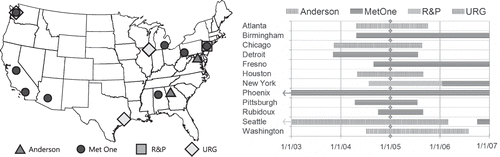
As shown in Figure 1, collocated IMPROVE and CSN samplers were operated at 12 urban sites for different time periods and with different CSN samplers. For this comparative analysis, only data from 2005 through 2006 are used, because in 2005 the carbon analyzers used by IMPROVE were upgraded, the precision of the CSN carbon concentrations improved after 2005, and after 2006 the U.S. EPA began changing the samplers and analytical methods used by the CSN for carbonaceous PM to be nearly identical to those used by IMPROVE, so the differences described here will not be applicable to more recent data.

Figure 1. Location of the 12 urban sites with collocated IMPROVE and CSN carbon measurements and the time period the samplers were operating.

The comparison of the total carbon (TC) concentrations from all collocated samplers is presented in Figure 2. As shown, CSN TC concentrations are generally higher than IMPROVE TC, with the magnitude of the difference dependent on the CSN sampler but independent of the monitoring site. This difference, or bias, has two components. One is additive, as evident by the positive intercept as the IMPROVE TC concentrations approach 0; the second is concentration-dependent, or multiplicative, as evident by the increasing difference with concentration. The additive bias varies by CSN sampler type and, though not shown in Figure 2, there is also a seasonal dependence, with a generally higher difference in the summer months compared to winter. The IMPROVE data have been corrected for an additive positive carbon artifact, whereas the CSN data have not. The additive bias in the CSN data is viewed as the positive organic carbon artifact associated with quartz filters.12,13

Figure 2. Comparison of CSN TC and IMPROVE TC concentrations from collocated monitors for 2005–2006 data. The data are color-coded based on the CSN sampler. The regression line is for the Met One data.

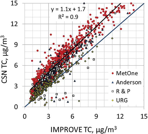
The difference also appears to be sampler-dependent, with the lowest differences for the URG sampler and highest for the Met One sampler, though the difference was not found to vary by season. One potential cause for these differences is that these samples are subject to a negative organic carbon artifact associated with the loss of SVOC, due to pressure differences across the filters. The IMPROVE sampler has the highest face velocity, thus the highest pressure drop, whereas the face velocity of the Met One sampler is an order of magnitude lower than IMPROVE, and URG's is between IMPROVE and Met One (Table 1). Other possible causes include different concentrations of SVOCs at the location of the monitoring site and different filter handling procedures. For example, CSN ships the filters cold whereas IMPROVE does not. Dillner et al.11 found that filters lost 10% of TC when maintained at temperatures at 40 °C for 96 hr. However, the lack of seasonal dependence in the multiplicative bias suggests that these are not the principal causes of the bias.

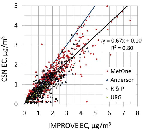
Figure 3 presents the comparison of the IMPROVE and CSN EC concentrations for collocated monitors. As shown, the IMPROVE EC concentrations are generally higher than the CSN EC. This difference is near 0 at low EC concentrations and increases with EC concentrations, indicating a multiplicative bias. The difference between CSN and IMPROVE EC dependencies is not dependent on the CSN sampler, suggesting that it is an analytical bias. Laboratory studies20 have shown that the NIOSH TOT method used for carbon measurements in the CSN results in lower EC and higher OC concentrations compared to the IMPROVE TOR method. The lack of an additive bias is supported by little to no EC measured on IMPROVE backup filters that are used to estimate the positive carbon artifact.13

Figure 3. Comparison of CSN EC and IMPROVE EC concentrations from collocated monitors for 2005–2006 data. The data are color-coded based on the CSN sampler. The regression line is for the Met One data.

Relating CSN to IMPROVE Carbon Concentrations

The TOR and TOT analytical analyses used in IMPROVE and the CSN have equivalent estimates of TC but different OC and EC subfractions.20 However, as discussed above, TC concentrations, reported from data collected using collocated samplers, differ. These differences apparently are due to the use of different sampling hardware and how known sampling artifacts are incorporated into reported data. In order to contrast and compare carbon concentrations derived from the IMPROVE and CSN monitoring networks, the CSN data are normalized or adjusted to account for the relative biases between sampling systems. This is done using data collected from collocated IMPROVE and CSN samplers. Each CSN sampler will necessarily have unique adjustment factors; however, only the Met One sampler has sufficient data for a statistical comparative analysis.

In this analysis, it is assumed that the TC concentrations measured from the filter samples differ from those in the atmosphere, due only to an additive positive organic carbon artifact resulting from filter adsorption of SVOC gases, and a multiplicative negative organic carbon artifact associated with volatilization of collected OC mass such that

(1)

where [TC] and [OC] are the actual ambient total and OC concentrations, respectively; [TC]^F is the TC concentration on the filter; B is the negative multiplicative sampling artifact; and A is positive additive artifact on the filter, represented as a concentration.

Because IMPROVE data-handling protocol calls for a correction for the positive artifact, it is assumed that A ^IMP = 0, and undoubtedly there is some volatilization of OC from both the CSN and IMPROVE samplers. However, because the existing routine monitoring data sets do not allow for the determination of B ^CSN, the strategy taken here is to normalize IMPROVE to CSN. Therefore B ^CSN is set to zero and B ^IMP is estimated relative to the CSN Met One sampler.

Under these assumptions, eq 1 for the reported IMPROVE and CSN TC concentrations becomes

(2)

(3)

If it is further assumed that it is [OC]^IMP and not [EC]^IMP that is volatilized and that the volatilization is proportional to organic mass concentration, then

(4)

Combining eqs 2 – 4, it can be shown that

(5)

Equation 5 relates the CSN TC concentrations to the IMPROVE EC and OC concentrations, with IMPROVE OC corrected for a negative artifact and the CSN TC corrected for the positive artifact.

The form of eq 5 lends itself to a statistical regression model of the form

(6)

where b _OC = (B ^IMP + (B ^IMP)²); a_i is the positive artifact, A ^CSN, for each month, i, of the year.

The ordinary least squares (OLS) regression resulted in a significant b _OC = 0.22 ± 0.03. A b _OC = 0.22 is equivalent to an IMPROVE multiplicative artifact B ^IMP = 0.19. This suggests that ∼20% of the OC collected by IMPROVE is lost due to the negative artifact. The OLS-derived CSN monthly positive organic artifacts for the Met One sampler are presented in Table 2. As shown, these artifacts are seasonal, with about a 1 μg/m³ artifact during the winter and 2 μg/m³ during the summer.

Table 2. The multiplicative artifact (1 + b _OC) and the monthly positive organic artifact (a) used to relate the CSN and IMPROVE carbon concentrations

	Met One
1 + b OC	1.2
a Jan	1.1
a Feb	1.3
a Mar	1.2
a Apr	1.4
a May	1.6
a Jun	1.7
a Jul	1.8
a Aug	1.9
a Sep	1.5
a Oct	1.2
a Nov	1.0
a Dec	1.1
Note : The units for the positive artifacts are μg/m^3 and 1 + b OC is unitless.

Converting CSN to IMPROVE Carbon Concentrations

As shown in Figure 3, the differences between the IMPROVE and CSN EC are approximately multiplicative. Therefore,

(7)

where m is the multiplicative factor relating the two EC measurements.

Solution of eq 7, using OLS, results in m = 1.3 ± 0.2. Therefore, the reported IMPROVE EC concentrations can be approximated by the CSN Met One data via

(8)

To approximate IMPROVE OC using CSN concentrations, eqs 6 and 8 can be combined such that

(9)

Incorporating eq 8 into eq 9 and rearranging gives

(10)

The adjusted CSN TC is then simply the sum of OC^CSN_adj and EC^CSN_adj:

(11)

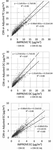
Figure 4 compares the CSN Met One carbon concentration to the reported IMPROVE concentrations for both the reported and adjusted CSN data. As shown, the adjustments of the CSN data significantly improve the comparison to the IMPROVE data. The positive intercepts for the reported TC and OC data are now near 0 for the adjusted data, and the slopes of the regression lines are near 1. The slope of the regression line for the EC data has also significantly improved from 0.68 to 0.89. In all cases the correlation between the data is high, with r ² ≥ 0.8.

Figure 4. The CSN and IMPROVE TC, OC, and EC concentrations for all collocated IMPROVE and CSN Met One samplers that collected data in 2005 and 2006. The lighter data points are for the reported CSN carbon concentrations and the darker data points are for the adjusted CSN carbon concentrations.

As evident by the remaining scatter between the IMPROVE and adjusted CSN data in Figure 4, the adjustments do not account for all variability between the CSN and IMPROVE carbon concentrations. In addition, the artifacts were derived using data from only five urban sites and may not be applicable to other sites and years. An alternative method for estimating the positive artifact is to regress the OC against ΔPM_2.5, where ΔPM_2.5 = PM_2.5 − inorganic compounds.13 The PM_2.5 mass on the Teflon filter would not have a positive OC artifact, so the regression intercept would be an estimate of the positive OC artifact. This was done using all CSN Met One data from 2000 to 2006 for each season, with winter comprising the months December–February. The resulting intercepts were approximately 1 μg/m³ for the winter, 2 μg/m³ for the summer, and 1.35 μg/m³ for the spring and fall, which are similar to those in Table 2. Although the average values are similar, there is some spatial variability in the intercept, with generally higher intercepts in California than the eastern United States. These results indicate that the derived artifacts in Table 2 are applicable to other years and sites but are most appropriate for examining aggregated data across multiple sites and time periods.

Comparison of Reconstructed to Measured Mass

In the CSN, five different samplers have been employed; however, about 75% were Met One samplers (Table 1). To minimize the influence of the different samplers, only samples collected using the Met One spiral aerosol speciation sampler (SASS) are used in the comparative analysis of reconstructed and gravimetric PM_2.5. Data collected between 2000 and 2008 are used in the CSN analysis, whereas data collected between 1988 and 2008 are used for the IMPROVE analysis. Where appropriate, CSN data are adjusted or calibrated to IMPROVE using eqs 8 and 10.

PM_2.5 and PM_2.5 species are often used in a closure-type calculation where assumed forms of aerosol mass species are added together and compared to gravimetrically measured PM_2.5. Even though ammonium concentrations are measured in the CSN, they will not be used in the following analysis. First, because ammonium is not routinely measured in the IMPROVE system, and second, unless volatilized ammonium is accounted for, which it is not in the CSN, the reported concentrations of ammonium can be significantly underestimated.22

The governing equation, assuming NH₄ concentrations are not measured, is

(12)

where

	RPM2.5 = reconstructed PM2.5 mass
	SO4 = sulfate ion concentration
	NO3 = nitrate ion concentration
	Roc = POM/OC
	POM = particulate organic matter
	OC = organic carbon concentration
	EC = elemental carbon
	Soil = oxides of crustal elements
	SS = sea salt
	D/D 0 = wet over dry particle diameter
	RH = relative humidity
	x = ammoniated sulfate to sulfate ion ratio, which varies from a minimum of 1.02 for sulfuric acid to a maximum of 1.375 for fully neutralized ammonium sulfate, a difference of about 30%.

PM_2.5 can be biased low because of volatilization of SVOCs and other volatile species such as ammonium nitrate or high because of retained water associated with inorganic salts and some water-soluble organic species. Typically, PM_2.5 concentrations are reported and used without correcting for these potential biases. In IMPROVE, SO₄ is usually assumed to be in the form of ammonium sulfate, which is an upper bound of mass associated with inorganic sulfate, the nitrate ion is assumed to be in the form of ammonium nitrate, and f′_salts is usually assumed to be 1, when in reality it is more likely to be between 1.15 and 1.3, assuming a laboratory RH between 30% and 40% and typical D/D ₀ factors at these RHs.23,24 Roc is usually assumed to be a constant between about 1.2 and 2.0, and the algorithms used to estimate soil and sea salt from elemental measured concentrations are assumed to be constant in both space and time.3

Some of these assumptions may have a seasonal dependence, such as sulfate ammoniation.25–35 Furthermore, it has been well documented that ammonium nitrate volatilization from a Teflon substrate is greater during the warmer summer season as opposed to cooler winter conditions.36–40 Nitrate volatilization as high as 90% in the summer and as low as 10% in the winter has been reported. However, even though more nitrate is retained on a fractional basis in the winter months, on an absolute basis the nitrate loss during the winter may be greater than summer.

Many authors have reported average Roc values that range from as low as 1.2 to values greater than 2.0.41–53 concluded that a factor of about 1.6 would be appropriate for an urban organic aerosol, whereas a factor of 2.1 may be more appropriate for an aged, nonurban aerosol.

A few authors have reported some seasonal dependence of Roc.53–58 Polidori et al.,57 using extraction/fractionation techniques, reported somewhat higher Roc values of 1.9–2.1 in the summer/winter for the Pittsburgh aerosol, probably because of a greater contribution of oxidized species.

Summing assumed forms of all species other than OC, subtracting this value from gravimetric PM_2.5, and assuming this value represents particulate organic matter (POM), Roc is estimated as POM/OC.52,53 This method of estimating Roc will be referred to as the mass difference technique (MDT). Chen and Yu,56 using a modified MDT for a Hong Kong data set, did not find any seasonal variability in Roc but did find the Roc was dependent on whether the air mass was “continental” or “marine”. Bae et al.,54 using an MDT for rural and urban New York data sets, reported a slight seasonal dependence for a nonurban site, with the warm season having a ratio of 2.1, whereas the urban site did not have a seasonal dependence but did have lower Roc factors of 1.3–1.6. Bae et al.55 used the MDT approach for a data set collected in St. Louis to estimate a Roc factor of 1.95 ± 0.17 in the summer and 1.77 ± 0.13 in winter. El-Zanan et al.53 reported on Roc factors derived from an Atlanta data set. They concluded that there was a slight seasonal difference in Roc, with a value of 1.77 in December and 2.39 in July. Lowenthal,58 using a Great Smoky Mountain National Park summer data set, reported Roc factors of 2.4 and 1.9 for water-soluble and dichloromethane extracts, respectively.

Figure 5 shows summary plots of gravimetric fine mass, sulfate as ammonium sulfate, nitrate as ammonium nitrate, soil as oxides of the soil elements, sea salt as 1.8·Cl, POM as 1.8·OC, and EC for IMPROVE and CSN urban and nonurban sites. CSN urban and nonurban sites were identified based on their classification in the U.S. EPA CSN database (http://www.epa.gov/ttn/airs/airsaqs/detaildata/downloadaqsdata.htm).

Figure 5. Stacked bar charts showing average concentrations of each species for all and each season for IMPROVE, CSN suburban, and CSN center city.

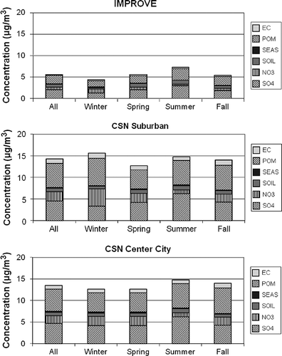
Notice that CSN total fine mass concentrations are about a factor of 3 times greater than in the IMPROVE network. This difference is undoubtedly in part due to the difference in urban/suburban and remote concentrations but also because most of the CSN sites are in the East, where regional sulfate concentrations are high, whereas IMPROVE sites are spread more uniformly across the country. There is also more seasonal variability in the IMPROVE data set, with concentrations being lowest in winter and highest during the summer months. Data for the suburban locations actually show the highest total concentrations during winter, primarily because of POM and nitrates. In the urban data set, winter and spring RPM_2.5 is about the same and lower than either summer or fall. Possibly, during winter months, during more stable and stagnant meteorological conditions, aerosols are more constrained to concentrate around the source areas, with less transport into the more remote locations where most IMPROVE monitors are located. Furthermore, nitrate and POM are a larger fraction of RPM_2.5 in urban locations, whereas in the IMPROVE network, soil, on a fractional basis, is elevated relative to CSN sites.

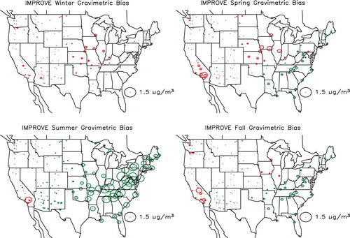
To see if there are systematic spatial and seasonal differences between reconstructed and gravimetric mass in the CSN and IMPROVE data sets, timelines of the percent difference between gravimetric and reconstructed PM_2.5, % ΔPM_2.5 = ((PM_2.5 − RPM_2.5)/PM_2.5) × 100, were plotted for each of the approximately 300 CSN and 170 IMPROVE sites. For these plots, it is assumed that x = 1.375 (fully neutralized ammonium sulfate), NH₄NO₃ = 1.29·NO₃, f′(RH) = 1, Roc = 1.8, sea salt = 1.8·Cl⁻, and Soil = 2.2[Al] + 2.49[Si] + 1.94[Ti] + 1.63[Ca] + 2.42[Fe]. An example plot of % ΔPM_2.5 is shown in Figure 6 in green for Brigantine National Wildlife Refuge.

Figure 6. Temporal plot of PM_2.5 − PM_2.5avg and the percent difference between reconstructed and gravimetric mass for Brigantine National Wildlife Refuge. The red line is a sinusoidal curve fit to the percent difference between reconstructed and gravimetric mass.

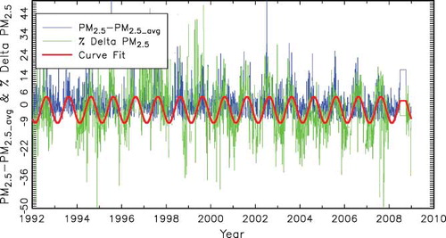
Also presented in Figure 6 in blue is a temporal plot of PM_2.5 − PM_2.5avg, where PM_2.5avg is the average PM_2.5 over the entire time period. Notice that there is a systematic seasonal bias in % ΔPM_2.5, with summer being biased high and winter low by as much as ±15%. Also notice that this bias tends to follow increases and decreases in PM_2.5 concentrations. Gravimetric mass, PM_2.5, is greater than RPM_2.5 during summer time periods, when PM_2.5 is high, and is lower than RPM_2.5 during winter months, when PM_2.5 is lower. It is also of interest to point out that the seasonal temporal trends in both PM_2.5 and % ΔPM_2.5 are more systematic after about 1999, possibly indicating a higher degree of precision in the post-1999 data set. The difference between pre- and post-1999 data is evident throughout the IMPROVE data set.

The seasonal variability exhibited in Figure 6 was modeled using a simple time-dependent cosine function relationship:

(13)

where T refers to time and f(T) was adjusted to yield a maximum and minimum during the summer and winter seasons, respectively. b ₁ and b ₂ are regression coefficients that have a physical interpretation of b ₁ being equal to the average positive or negative percent bias, whereas b ₂ is the average percent variability between summer and winter.

The red line in Figure 6 is the curve fit of eq 13 for the data shown, giving b ₁ = −4.3 and b ₂ = 16.4, implying that on the average PM_2.5 is 4.3% lower than RPM_2.5 and there is an average difference between summer and winter of 16.4%. The t statistic for this site was 15.1, indicating a high level of significance.

This analysis was carried out for each site in both the IMPROVE and CSN networks. Only coefficients with t values greater than 1.7 are reported. Figure 7 shows the percent variability, b ₂, between the summer and winter seasons and the average bias, b ₁, for the IMPROVE and CSN networks.

Figure 7. Average percent seasonal variability (b ₂) and percent difference (b ₁), as represented by eq 13, between reconstructed and gravimetric mass for the IMPROVE and CSN monitoring networks. Green represents a positive value, whereas red represents a negative bias.

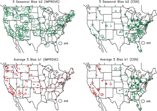
The number of observations varies significantly from site to site, especially in the CSN, where site start dates vary considerably. Of the 168 sites with t values greater than 1.7, about 30% have 100–300 observations, whereas another 40% of the sites have 300–500 data points. A few sites have as many as 900 observations. In the IMPROVE network, 80% of the monitoring sites have over 800 observations. Therefore the statistical significance of the bias estimations presented in Figure 7 varies from site to site and should be viewed as being semiquantitative. All sites were included in the analysis to elucidate possible spatial and seasonal trends across the spatial and temporal scales that these networks represent.

A statistical summary of seasonal variability and average bias is presented in Table 3 for all IMPROVE and CSN sites. Referring to Table 3 and Figure 7, notice that the seasonal variability in the IMPROVE network is on the average about twice as high as in the CSN, with average values of 14.9% and 7.6%, respectively. The maximum value of seasonal variability is also higher for the CSN.

Table 3. Summary of the percent seasonal variability and average difference of reconstructed versus gravimetric mass

Variable	Mean	SD	Minimum	Maximum	N
Seasonal variability (IMPROVE)	14.9	6.14	0.0	26.7	158
% Seasonal variability (CSN)	7.6	4.51	0.0	19.0	168
Average difference (IMPROVE)	−3.9	4.44	−17.9	9.4	158
Average difference (CSN)	3.4	7.00	−17.7	22.7	168

Interestingly, almost all sites exhibit some seasonal dependence of % ΔPM_2.5. There are some qualitatively consistent spatial patterns that emerge from both networks. The high plateau (Mogollon Rim) region of northern Arizona and New Mexico and a region extending down into Texas (Big Bend National Park) have lower seasonal variability, as do areas of the northern California Sierra Nevada mountains. Generally, the upper Midwest and parts of Florida also have low seasonal variability. The Columbia River Gorge and Snake River valley have high variability, with lower values to the immediate north and south.

Figure 7 also shows the overall average percent bias, b ₁, for the IMPROVE and CSN networks. Red symbols indicate that the average bias is negative (PM_2.5 < RPM_2.5), whereas green symbols represent a positive bias (PM_2.5 > RPM_2.5). Referring to the map for IMPROVE, notice that except for a few sites in the West, in the IMPROVE network reconstructed mass is greater than gravimetric mass. This is especially true in the warm Southwest and Southern California, where nitrate mass concentrations are high relative to other species, suggesting nitrate volatilization from the Teflon filter on which gravimetric analysis is performed. Referring to the map for the CSN, one can see that RPM_2.5 > PM_2.5 in almost every urban/suburban area in the West, whereas RPM_2.5 < PM_2.5 in almost every urban/suburban site in the East. Notice the very interesting dichotomy between the rural/remote and urban/suburban sites in the East. On the average, RPM_2.5 is an underestimate of PM_2.5 by about 4% and an overestimate of about 3% in the IMPROVE and CSN networks, respectively.

The average biases and seasonal variability in % ΔPM_2.5 could have significant ramifications. In the RHR guidance, it is recommended that reconstructing extinction, the parameter used to determine whether progress is being made toward improvement of visibility in Class I areas, is based on the assumption that days with high PM_2.5 concentrations have average mass size distributions that are more conducive to efficient scattering of light. The high-concentration days tend to occur during summer months, and possibly all or part of this observed relationship between increased scattering on higher-concentration days is a result of assuming an Roc, the level of sulfate ammoniation, or an assumed molecular form of other species is constant, when in fact one or more may have significant seasonal variability.

Furthermore, interpreting PM_2.5 as it relates to health endpoints may be problematic. The bias associated with gravimetric mass determinations varies from one region of the country to the other. For instance, in the Midwest where nitrate makes up a significant fraction of PM_2.5, if 70% of the nitrate is volatilized and nitrate contributed 80% of the PM_2.5, then PM_2.5 would be underestimated by 56%. Likewise, if SO₄ were 80% of PM_2.5, more than 20% of reported mass would be due to water on the hygroscopic species.

INVESTIGATING BIAS ASSOCIATED WITH EACH SPECIES

Differences between gravimetric and reconstructed mass are a function of the difference between the gravimetric and assumed mass of each species. The differences between species-by-species PM_2.5 and RPM_2.5 are given by

(14)

where Other is the sum of elemental carbon (EC), sea salt, and soil dust.

PM_{2.5 i} refers to the various species on the Teflon filter from which gravimetric mass is determined, RFM_{2.5 i} refers to the individual derived or reconstructed species mass. The remaining variables are defined in eq 12. Each of the terms in the parentheses contributes to either a positive or negative bias between PM_2.5 and RPM_2.5.

The relationship between PM_2.5 and aerosol species concentrations can be explored with a regression model of the form

(15)

where Other = Soil + EC+ sea salt; a_i = the regression coefficients.

The regressions were carried out for all data (across all sites) collected in the IMPROVE monitoring network and for the data set subdivided into seasons. The same analysis was carried out using CSN data after they had been subdivided into urban and suburban categories. Results of these analyses are presented in Tables 4a–4c.

Table 4a. Results of OLS regression analysis using eq 15 for the IMPROVE monitoring data

Variable	Estimate	SE	t value	Probability of >|t |
All
R ^2 = 0.95
ASO4	1.12	0.00	1328.90	0.00
ANO3	0.75	0.00	410.67	0.00
POM	1.60	0.00	822.62	0.00
Other	1.06	0.00	597.08	0.00
Winter
R ^2 = 0.96
SO4	1.02	0.00	391.99	0.00
NO3	0.92	0.00	403.37	0.00
POM	1.42	0.00	301.41	0.00
Other	1.05	0.00	234.18	0.00
Spring
R ^2 = 0.93
SO4	1.10	0.00	560.18	0.00
NO3	0.70	0.00	200.96	0.00
POM	1.52	0.00	344.45	0.00
Other	1.09	0.00	402.66	0.00
Summer
R ^2 = 0.96
SO4	1.15	0.00	793.24	0.00
NO3	0.51	0.01	47.14	0.00
POM	1.70	0.00	465.24	0.00
Other	1.08	0.00	295.10	0.00
Fall
R ^2 = 0.96
SO4	1.09	0.00	696.73	0.00
NO3	0.75	0.00	206.21	0.00
POM	1.59	0.00	467.48	0.00
Other	1.06	0.00	273.71	0.00

Table 4b. Results of OLS regression analysis using eq 15 for the CSN/suburban monitoring data

Variable	Estimate	SE	t value	Probability of >|t |
All
R ^2 = 0.96
SO4	1.23	0.00	412.51	0.00
NO3	0.94	0.00	237.83	0.00
OC	1.52	0.01	230.17	0.00
Other	1.16	0.01	111.73	0.00
Winter
R ^2 = 0.92
SO4	1.22	0.01	109.01	0.00
NO3	1.04	0.01	151.13	0.00
OC	1.41	0.01	110.58	0.00
Other	1.10	0.03	42.38	0.00
Spring
R ^2 = 0.89
SO4	1.20	0.01	155.65	0.00
NO3	0.90	0.01	118.87	0.00
OC	1.53	0.01	107.78	0.00
Other	1.31	0.02	70.84	0.00
Summer
R ^2 = 0.93
SO4	1.19	0.01	230.61	0.00
NO3	0.77	0.02	47.88	0.00
OC	1.77	0.01	125.08	0.00
Other	1.23	0.02	58.29	0.00
Fall
R ^2 = 0.94
SO4	1.20	0.01	216.18	0.00
NO3	0.96	0.01	126.32	0.00
OC	1.43	0.01	114.22	0.00
Other	1.14	0.02	62.40	0.00

Table 4c. Results of OLS regression analysis using eq 15 for the CSN/urban monitoring data

Variable	Estimate	SE	t value	Probability of >|t |
All
R ^2 = 0.90
SO4	1.25	0.00	370.11	0.00
NO3	0.97	0.00	197.57	0.00
OC	1.44	0.01	233.14	0.00
Other	1.07	0.01	102.34	0.00
Winter
R ^2 = 0.94
SO4	1.25	0.01	100.28	0.00
NO3	1.06	0.01	128.23	0.00
OC	1.33	0.01	96.02	0.00
Other	1.04	0.03	38.43	0.00
Spring
R ^2 = 0.880
SO4	1.24	0.01	139.37	0.00
NO3	0.93	0.01	87.96	0.00
OC	1.34	0.02	86.97	0.00
Other	1.22	0.02	62.96	0.00
Summer
R ^2 = 0.93
SO4	1.23	0.01	217.79	0.00
NO3	0.71	0.03	20.50	0.00
OC	1.61	0.01	155.65	0.00
Other	1.23	0.02	62.47	0.00
Fall
R ^2 = 0.91
SO4	1.24	0.01	197.59	0.00
NO3	0.98	0.01	101.19	0.00
OC	1.39	0.01	112.29	0.00
Other	1.00	0.02	50.08	0.00

 

The coefficients in the regression model represented by eq 15 have physical interpretations. a ₁·1.375·SO₄ is PM_{2.5 SO4}, or the sulfate plus water mass on the Teflon substrate used to determine gravimetric mass. Therefore, for fully neutralized sulfate one would expect a ₁ to be greater than 1 and 1 − a ₁ to be the fraction of sulfate mass that is particle-bound water. However, a ₁ is an upper bound because sulfate may not be fully neutralized, and the regression coefficient a ₁ will necessarily be decreased to reflect the difference between the assumed fully neutralized sulfate and sulfate mass actually contributing to gravimetric mass.

a ₂·1.29·NO₃ is interpreted as the nitrate mass plus water as measured on the Teflon filter used for gravimetric analysis (PM_2.5 NO₃). This value includes the nitrate not volatilized from the Teflon filter as well as bound water on the nitrate aerosol. Assuming that 1 − a ₁ is also a representation of the mass fraction of water associated with nitrate aerosol, then 1 − a ₂/a ₁ is an approximation of the fraction of nitrate volatilized from the Teflon filter, assuming that sulfate was fully neutralized.

a ₃·1.8 is the Roc factor, assuming that POM collected on the Teflon and quartz substrates is the same. The OC^CSN data were adjusted according to eq 9 to account for the differences between TOT and TOR but were not adjusted for the volatilization loss associated with the IMPROVE sampling system. The Roc factors associated with the Met One and IMPROVE samplers could be different for the same ambient POM aerosol because of preferential volatilization of some POM species.

The annual and seasonal estimates for the fractional increase in sulfate mass due to water retention, fraction of nitrate lost from the Teflon filter, and Roc factor for IMPROVE and CSN urban and suburban sites are summarized in Figures 8–10. Referring to Figure 8, notice that water retention is on the order of 1.2–1.25 for center city/suburban sites. This range of fractional retention of water is consistent with measured and theoretical values of D/D ₀ ratios of about 1.05–1.1 or an increase of mass of about 15–30% at 30–40% RH. It is greatest at center city sites and decreases as one moves to suburban and rural/remote areas. There is very little seasonal dependence for the center city/suburban sites but a very pronounced seasonal dependence for the rural/remote IMPROVE sites. There is little predicted water retention during the winter months, whereas during the summer season the water retention factor is 1.15. The difference between times when sulfates retain water at the low RH found in the laboratory may be due to sulfate neutralization and the mixing characteristics of urban aerosols. Sulfates during winter months tend to be more neutralized than during the summer and may not have deliquesced and therefore retain little water. Furthermore, measurements in the eastern areas of the United States, where most CSN monitors are located, show f(RH) and D/D ₀ functions that have continuous growth curves showing neither deliquescence or crystallization characteristics.59–61

Figure 8. Average fractional increase in sulfate and nitrate mass, a ₁, due to retained water for the IMPROVE and CSN monitoring networks.

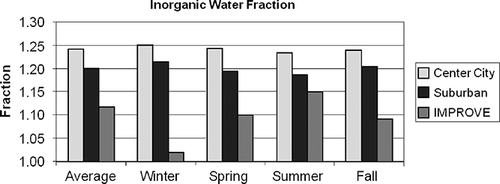
Figure 9. Average fraction of nitrate volatilized from a Teflon filter, (1 − a ₂/a ₁), for the IMPROVE and CSN monitoring networks.

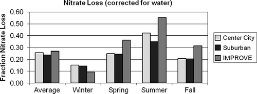
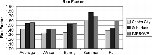
Figure 10. Average Roc factor, a ₃, for the IMPROVE and CSN monitoring networks.

Estimated seasonal variability of nitrate volatilization from a Teflon filter is consistent with reported values. In Figure 9, winter fractional loss of nitrate is about 10%, whereas during the summer the average loss is estimated to be 40–50%, with spring and fall loss being intermediate compared to summer/winter. There is very little difference of nitrate volatilization between urban and suburban sites.

Figure 10 shows that there is a rather dramatic seasonal difference in Roc factors, with winter and summer being at about 1.3–1.4 and 1.6–1.8, respectively. Spring and fall have intermediate values as compared to winter/summer. Because of less photochemistry during winter months, one might expect POM to be less oxygenated and have lower Roc factors than summer months. Also, because urban areas are likely sources of OC, it might be expected that a “young” urban organic aerosol would have a lower Roc factor than a more aged rural or remote aerosol. Figure 10 shows that these differences, if they exist, are not large. The center city Roc factors are systematically lower than either suburban or rural sites but only by about 5–15%. Interestingly, suburban and rural Roc factors are about the same. Because the Roc factors between IMPROVE and CSN Met One monitoring systems are nearly the same, in spite of a 20% loss of OC using the IMPROVE system, it seems reasonable to hypothesize that the Roc factor of the volatilized SVOC is about the same as the OC that is retained.

Using the regression results summarized in Tables 4a–4c, it is possible to assess the average difference between PM_2.5 and RPM_2.5 as a function of species as represented by eq 14 and shown for one location in Figure 6. Typically, PM_2.5 − RPM_2.5 cycles between having its highest and lowest values during the summer and winter, respectively. Figures 11–13 show the combined difference (PM_2.5 − RPM_2.5) and the difference associated with each species for the IMPROVE network and for the CSN, subdivided into center city and suburban, as a function of season.

Figure 11. The estimated average difference between gravimetric and assumed forms of the various aerosol species contributing to PM _2.5 for IMPROVE. The differences are estimated as 1.375·SO₄ × (a ₁ − 1), 1.29·NO₃ × (a ₂ − 1), OC × (a ₃ − 1.8), and Other × (a ₄ − 1) for sulfates, nitrates, organics, and Other, respectively.

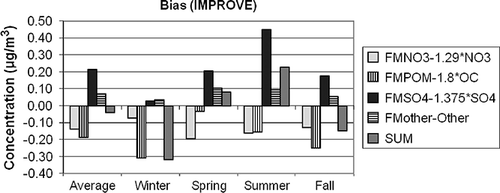
Figure 12. The estimated average difference between gravimetric and assumed forms of the various aerosol species contributing to PM _2.5 for CSN center city. The differences are estimated as 1.375·SO₄ × (a ₁ − 1), 1.29·NO₃ × (a ₂ − 1), OC × (a ₃ − 1.8), and Other × (a ₄ − 1) for sulfates, nitrates, organics, and Other, respectively.

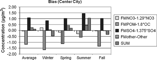
Figure 13. The estimated average difference between gravimetric and assumed forms of the various aerosol species contributing to PM _2.5 for CSN suburban. The differences are estimated as 1.375·SO₄ × (a ₁ − 1), 1.29·NO₃ × (a ₂ − 1), OC × (a ₃ − 1.8), and Other × (a ₄ − 1) for sulfates, nitrates, organics, and Other, respectively.

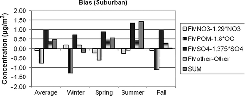
First, notice that the scale of the ordinate axis on the IMPROVE and CSN graphs are different in that the range of values for IMPROVE is −0.4 to +0.5 µg/m³, whereas for the CSN graphs it is −2.0 to +2.0 µg/m³, reflecting the higher aerosol concentrations in urban/suburban areas. On the average the difference between PM_2.5 and RPM_2.5 is only a few percent, at 1.5% and 4% for urban and suburban, respectively, and 3% for IMPROVE. These overall average low differences between PM_2.5 and RPM_2.5 suggest a false sense of certainty as to the chemical characteristics of individual species, as well as the confidence in gravimetric mass levels. It is evident from Figures 11–13 that there are compensating uncertainties or errors both in the species differences and in temporal or seasonal difference characteristics.

The two largest average differences are in sulfate and POM mass. The temporal trend of the difference for both species is the same in that the difference is lowest in winter and highest during the summer months. However, the sulfate difference is always positive, whereas the POM difference is always negative. In the IMPROVE network, the water/sulfate difference is near 0 during the winter months and approaches 0.5 µg/m³ during the summer, which is about 6% of the gravimetric mass and about 16% of the sulfate mass. Both center city and suburban water/sulfate differences vary from near 0.5 to 1.5 µg/m³ during winter and summer, respectively. On a percentage basis, this is about 3–10% of gravimetric mass and 15–25% of ammonium sulfate mass.

In the IMPROVE network, POM difference varies from −0.35 µg/m³ (−20%) to −0.15 µg/m³ (−5%) during the winter and summer months, respectively. The POM winter difference for center city is about −1.5 µg/m³ (−40%) for the winter, whereas the summer difference is −0.5 µg/m³ (−16%). The average POM suburban difference is about the same as center city for the winter months but is only −0.08 µg/m³ (−3%) for summer months. The implication here is that an Roc factor of 1.8 may be, on the average, a bit high for the higher-POM-concentration summer months but substantially high for the lower-concentration time periods, which correspond to the winter season.

Nitrate difference has the opposite seasonal trend in that the difference is lowest in winter months and highest during summer, when ambient temperatures are higher and therefore conducive to more ammonium nitrate volatilization. The average difference across the IMPROVE network during the winter is −0.08 µg/m³ (9%), whereas during the summer it is −0.17 µg/m³ (56%). There is little variation in nitrate difference between center city and suburban. In both the center city and suburban data sets, the wintertime nitrate difference is on the order of 0.25 µg/m³ (4–6%), whereas during the summer it is about −0.25 µg/m³ (−25%). Even though nitrate is volatilized from the PM Teflon filter during the winter season, the nitrate plus bound water on the Teflon filter is greater than nitrate alone on the nylon filter. During the summer there is enough nitrate volatilized from the Teflon filter such that the nitrate plus particle-bound nitrate water is substantially less than the nitrate collected on the nylon substrate.

Other (sea salt + EC+ soil) also has systematic seasonal differences, although they are harder to interpret. It is assumed that sea salt is represented by 1.8·Cl. This could be an over- or underestimate, depending on the aging and reactions that a sea salt aerosol has undergone and the assumed form of oxides of the elements that make up the “soil” fraction. For instance, the elemental composition, internationally transported dust is different from that found in the desert Southwest and, for that matter, anywhere in the continental United States. The “correction” or regression factors were on the order of 1.04–1.08 for IMPROVE and a bit higher for CSN data, at about 1.2, indicating that Other has been underestimated by about 10–20%.

Bias in Gravimetric Mass

Having an approximate understanding of the difference between measured and reconstructed mass concentrations, it is possible, with some assumptions, to develop over- or underestimates of the policy-relevant variables as they relate to PM_2.5 NAAQS and the RHR. First, it must be pointed out that the above analysis does not establish the bias associated with volatilization of SVOCs from various filter media as a function of sampler design and physical characteristics. However, it was shown that OC collected using the IMPROVE sampling system is systematically about 20% lower than OC collected using the Met One sampler and that the difference may be in part due to filter face velocity. This suggests that all samplers have some inherent loss of semivolatile species, although the amount cannot be quantified with the data sets that are currently routinely collected.

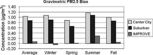
The average difference between PM_2.5 gravimetric mass and true ambient mass (TPM_2.5) concentration is estimated by assuming that POM, crustal material, and sea salt gravimetric mass are measured without bias and that the positive difference due to retained water on the nitrate and sulfate aerosol at the time of filter weighing and nitrate loss due to volatilization can be estimated using regression coefficients a ₁ and a ₂:

These results are summarized in Figure 14 for the IMPROVE and the center city and suburban CSN data sets. The difference associated with nitrate volatilization from the Teflon filter is compensated for by retained water on the hygroscopic inorganic species. The only time when nitrate volatilization is greater than retained water mass is during the winter season in the IMPROVE network, when the average PM_2.5 mass is underestimated by less than 0.1 µg/m³. The average difference for the IMPROVE data set is 0.07 µg/m³ or about 1%. The maximum difference occurs during the summer season and is about 0.3 µg/m³ or 4%. The difference associated with the CSN data set is nearly the same for all seasons and always positive at about 0.8–1.2 µg/m³, which is about 6%. These values are well within measurement uncertainty.

Figure 14. Average difference between gravimetric and estimated true PM_2.5 mass concentration for the IMPROVE and CSN data sets (see eq 16).

Bias in Reconstructed Mass

The sum of biases shown in Figure 15 associated with OC and Other can be used to estimate the average difference of reconstructed PM_2.5 relative to TPM_2.5 concentrations:

Figure 15. Average difference between reconstructed and estimated true PM_2.5 concentrations for the IMPROVE and CSN data sets (see eq 17).

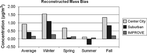
The bias of assuming sulfates are fully neutralized is not addressed, nor are differences associated with assuming all nitrates are in the form of ammonium nitrate. Furthermore, eq 17 implicitly assumes that, after correction for positive artifacts associated with the quartz substrate that is used in the OC TOT/TOR analysis, the volatilization (negative artifact) of SVOCs from the Teflon substrate used in the gravimetric analysis and quartz filter used in OC determination is the same.

Figure 15 shows the estimated overall average and seasonal differences between reconstructed and TPM_2.5. The average overall difference for the IMPROVE data set is 0.2 µg/m³, or about 3.5%. The average differences for the center city and suburban sites are 0.9 and 0.4 µg/m³, respectively. These values correspond to 7% and 3% of measured fine mass. The greatest difference occurs during the winter season, primarily because POM is overestimated (see Figures 11–13). The winter difference for IMPROVE is 0.3 µg/m³, whereas for center city and suburban sites it is 1.6 and 1.1 µg/m³, respectively. These values correspond to about a 7% difference for IMPROVE and suburban sites and about a 10% difference for center city data. The least difference occurs during the summer months, when it is on the order of only 1% or 2%. Differences for the spring and fall seasons are intermediate to winter and summer.

SPATIAL AND SEASONAL VARIABILITY IN PM_2.5 AND RPM_2.5 BIASES

The approximate seasonal and spatial variability in CSN and IMPROVE fine gravimetric and reconstructed fine mass biases can be explored by applying the regression coefficients a ₁, a ₂, a ₃, and a ₄ derived from the CSN and IMPROVE seasonal data sets for all sites to the site-specific sulfate, nitrate, POM, and Other concentration averages. Alternatively, regressions could be carried out using site-specific data; however, because of an insufficient number of data points, the regression coefficients can be highly variable with large standard errors. It is recognized that the regressions using the site-combined data sets may not be entirely representative of physical and chemical processes that might occur on a site-specific basis. However, they will capture the implications of seasonal variability in aerosol mix that occurs on a site-by-site basis.

Figure 16 shows the spatial distribution in the estimated difference between gravimetric and true mass concentration (PM_2.5 − TPM_2.5) for the combined urban/suburban data sets as a function of season, whereas Figure 17 shows the same information for the IMPROVE data set. The circles are color-coded so that green and red correspond to gravimetric mass being greater or less than true mass. First of all, notice that for both data sets the differences associated with the West, except for Southern California, are lower than for the eastern United States. Furthermore, the central-eastern United States has the highest difference at about 1.5–2.0 µg/m³ for the CSN and for the summer months in the IMPROVE network. The positive difference is associated with retained water on an aerosol primarily made up of sulfate. This sulfate-driven positive difference in the eastern United States should be compared to Southern California, where during the summer there is a greater than 1.5 µg/m³ negative difference in both networks. In the IMPROVE network there is a negative difference in gravimetric mass at nearly all monitoring sites during the winter and spring months, when sulfate concentrations are lowest and nitrate concentrations the highest. The negative difference corresponds to volatilization of a nitrate-dominated ambient aerosol.

Figure 16. Seasonal and spatial variability in difference between gravimetric and true mass concentration (PM_2.5 − TPM_2.5) for the CSN monitoring network. Green color refers to positive and red to negative numbers.

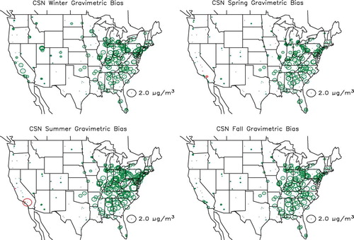
Figure 17. Seasonal and spatial variability in difference between gravimetric and true mass concentration (PM_2.5 − TPM_2.5) for the IMPROVE monitoring network. Green color refers to positive and red to negative numbers.

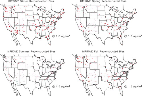
Figure 18 shows the spatial and seasonal distribution in the variability between true and reconstructed mass concentration (TPM_2.5 − RPM_2.5) for the CSN combined urban/suburban data sets, whereas Figure 19 shows the same information for the IMPROVE data set. Circles coded red correspond to reconstructed mass being greater than ambient mass concentration. In both data sets the negative difference is greatest in the winter and lowest in the summer months. This difference is primarily associated with an assumed Roc factor used to estimate POM from measured OC that is too high during winter months and about right during summer. As shown in Figure 10, the Roc factor was shown to vary from about 1.4 during the winter months to near 1.8 in the summer, and the Roc factor used in estimating reconstructed mass concentrations for all months was 1.8. It should also be noted that during the winter there are negative-difference “hot spots” around western urban areas. These hot spots correspond to elevated concentration levels of OC in urban areas such as Phoenix, Arizona, Spokane, Washington, the California San Joaquin valley, and the south coast air basin in California that are located in valleys and basins where wintertime emissions are trapped by shallow mixing heights.

Figure 18. Seasonal and spatial variability in difference between true and reconstructed mass concentration (TPM_2.5 − RPM_2.5) for the CSN monitoring network. Green color refers to positive and red to negative numbers.

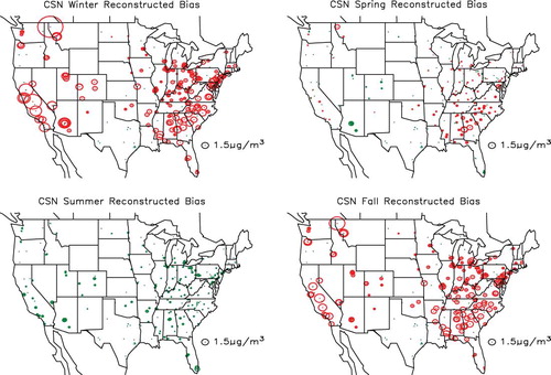
Figure 19. Seasonal and spatial variability in difference between true and reconstructed mass concentration (TPM_2.5 − RPM_2.5) for the IMPROVE monitoring network. Green color refers to positive and red to negative numbers.

SUMMARY

The NAAQS guideline for PM_2.5 is based on a gravimetric analysis of particulate matter collected on a Teflon substrate using federal reference methodologies. To help understand which of the many aerosol species contribute to elevated levels of PM, the U.S. EPA and the states also operate the CSN at approximately 200 sites. Filter substrates collected in the CSN are analyzed for gravimetric mass, inorganic ions, carbon, and elements. The IMPROVE monitoring program is operated to meet the needs of the Regional Haze Program, which is mandated to track long-term temporal changes in visibility in certain protected visual environments such as national parks and wilderness areas. The IMPROVE monitoring program is similar to the CSN, with exceptions being the sampling system hardware used to collect the aerosols, some filter handling protocols, and some quality assurance procedures. Only one type of sampling system is used throughout the IMPROVE monitoring network, whereas five systems have been used in the CSN, all of which are different from the IMPROVE system. Compliance under the RHR is based on reconstructed aerosol mass and light extinction from aerosol composition. Anions, OC, and elements are measured, and aerosol species concentrations are estimated assuming molecular forms of sulfates, nitrates, POM, sea salt, and soil dust.

Both measured and reconstructed mass have inherent biases. Compliance monitoring for PM_2.5 mass concentrations relies on a gravimetric analysis of aerosols that have been collected on a Teflon filter, whereas reconstructed mass is estimated from the sum of aerosol species that contribute to PM, assuming an average molecular form of those species. Collection of aerosols on a Teflon substrate results in volatilization of semivolatile species such as ammonium nitrate and some organic species, which corresponds to an overall loss of mass or negative artifact. These losses are to some degree compensated for when the filters are weighed in environments where the RH is 30–40%. Hygroscopic species can retain significant amounts of water at these RHs. For instance, sulfate and nitrate mass may be increased by as much as 30% due to retained water.

On the other hand, the aerosol species used in reconstructed mass are derived from assumed forms of sulfates, nitrates, OC, and soil dust. Typically, sulfates and nitrates are assumed to be fully neutralized by ammonium, a POM to OC ratio is assumed, and a form of oxides of soil-related elements is assumed. Furthermore, it is assumed that EC as derived from TOR/TOT is elemental and does not have other carbon compounds associated with it. It is known that all these assumptions can be violated at times.

A regression analysis between PM_2.5 and the assumed mass concentrations of derived aerosol species allows for an estimation of how each of the major aerosol species contributes to differences between PM_2.5 and RPM_2.5, and with certain assumptions, the bias from true mass in gravimetric and reconstructed mass concentration estimates.

First of all, it was demonstrated that there is on the order of a 20% difference in OC mass, depending on which sampling system was used. It is suggested that this loss may be associated with volatilization of SVOCs and may be dependent on filter face velocity. This implies that there may be some loss of SVOCs from all sampling systems; however, the specific loss as a function of sampler characteristics cannot be addressed with data that are routinely collected in the IMPROVE and CSN monitoring programs.

Assuming that the gravimetric mass of POM, crustal material, and sea salt is measured without bias and that the positive bias due to retained water at the time of filter weighing and nitrate loss due to volatilization can be estimated from the regression analysis, the overall difference between gravimetrically determined and true ambient fine mass was estimated. On the average, the difference is about the same for the urban and suburban data sets at about 1 µg/m³ or 6%. The average difference for the IMPROVE data set is 0.1 µg/m³ or 4%. The biggest difference for the IMPROVE data set occurs during the summer at 0.3 µg/m³, whereas for the CSN data sets, both summer and winter have the greatest bias at 1.0 µg/m³, with spring and fall having somewhat intermediate differences at 0.6–0.8 µg/m³.

Differences between reconstructed and true ambient mass concentrations associated with assumed molecular forms of species used in the RHR guidelines were estimated by assuming that sulfates and nitrates are accurately speciated and that the gravimetrically determined mass of POM, EC, sea salt, and soil dust accurately reflects these species' true mass. It was further assumed that, after correction for positive artifacts associated with the quartz substrate that is used in the OC TOT/TOR analysis, the volatilization (negative artifact) of SVOCs from the Teflon substrate used in the gravimetric analysis and the quartz filter used for OC determination is the same. Under these assumptions, the average overall difference between reconstructed and true mass for the IMPROVE data set is 0.2 µg/m³, or about 3.5%. The average differences for the center city and suburban sites are 0.9 and 0.4 µg/m³, respectively. These values correspond to 7% and 3% of measured fine mass. The greatest difference occurs during the winter season, primarily because of POM overestimation. The winter difference for IMPROVE is 0.3 µg/m³, whereas for center city and suburban sites it is 1.6 and 1.1 µg/m³, respectively. These values correspond to about a 7% difference for IMPROVE and suburban sites and about a 10% difference for center city data. The least difference occurs during the summer months, when the difference is on the order of only 1% or 2%. Differences for the spring and fall seasons are intermediate to winter and summer.

Fine gravimetric mass concentration bias in the western United States, except for Southern California, is lower than the eastern United States, and the central-eastern United States has the highest bias at about 1.5–2.0 µg/m³ for both networks. The positive bias is associated with retained water on an aerosol primarily made up of sulfate. This sulfate-driven positive bias in the eastern United States should be compared to Southern California, where during the summer there is a greater than 1.5 µg/m³ negative bias in both networks, primarily associated with a region of the country where ambient nitrate concentrations are high and nitrate volatilization becomes the biggest contributor to gravimetric mass concentration bias. In the IMPROVE network, there is a negative bias in gravimetric mass at nearly all monitoring sites during the winter and spring months.

Negative differences in reconstructed and estimated true mass concentrations in both the CSN and IMPROVE data sets are greatest in the winter and lowest in the summer months. These differences are primarily associated with an assumed Roc factor that is too high during winter months and about right during summer. The derived Roc factor is about 1.4 during the winter months to near 1.8 in the summer. Furthermore, there are negative-bias “hot spots” linked to western urban areas. These hot spots correspond to elevated concentration levels of OC in western urban areas that are located in valleys and basins, where wintertime emissions tend to be trapped by shallow mixing heights.

DISCLAIMER

The assumptions, findings, conclusions, judgments, and views presented herein are those of the authors and should not be interpreted as necessarily representing the National Park Service or National Oceanic and Atmospheric Administration policies.

REFERENCES

- Clean Air Status and Trends Network http://www.epa.gov/ttn/amtic/speciepg.html (http://www.epa.gov/ttn/amtic/speciepg.html) (Accessed: 5 April 2010 ).
- U.S. Environmental Protection Agency . March 1998 . SLAMS/NAMS/PAMS: Network Review Guidance, EPA-454/R-98-003 , March , Research Triangle Park , NC : Office of Air Quality, Planning and Standards .
- Malm , W.C. , Sisler , J.F. , Huffman , D. , Eldred , R.A. and Cahill , T.A. 1994 . Spatial and Seasonal Trends in Particle Concentration and Optical Extinction in the United States . J. Geophys. Res. , 99 : 1347 – 1370 .
- Regional Haze Regulations . 1999 . Fed. Regist. , 64 : 35714 – 35774 . Code of Federal Regulations, Part 51, Title 40, 1999
- U.S. Environmental Protection Agency. PM2.5 and Chemical Speciation—Speciation—Laboratory Standard Operating Procedures http://www.epa.gov/ttnamti1/specsop.html (http://www.epa.gov/ttnamti1/specsop.html) (Accessed: 5 April 2010 ).
- Frank , N.H. 2006 . Retained Nitrate, Hydrated Sulfates, and Carbonaceous mass in Federal Reference Method Fine Particulate Matter for Six Eastern U.S. Cities . J. Air Waste Manage. Assoc. , 56 : 509 – 511 .
- Chow, J.C.; Watson, J.G.; Chen, L.-W.A.; Rice, J.; Frank, N.H. Quantification of PM2.5 Organic Carbon Sampling Artifacts in US Networks; Atmos. Chem. Phys. 2010, 10, 5223–5239. http://www.atmos-chem-phys.net/10/5223/2010/acp-10-5223-2010.pdf (http://www.atmos-chem-phys.net/10/5223/2010/acp-10-5223-2010.pdf)
- Malm , W.C. , Schichtel , B.A. , Pitchford , M.L. , Ashbaugh , L.L. and Eldred , R.A. 2004 . Spatial and Monthly Trends in Speciated Fine Particle Concentration in the United States . J. Geophys. Res. , 109 : D0336 doi: 1029/2003JD003739
- Hand, J.L.; Malm, W.C. Review of the IMPROVE Equation for Estimating Ambient Light Extinction Coefficients; Cooperative Institute for Research in the Atmosphere (CIRA), ISSN 0737-5352-71; Colorado State University: Fort Collins, Colorado, March 2006 http://vista.cira.colostate.edu/improve/Publications/GrayLit/016_IM PROVEeqReview/IMPROVEeqReview.htm (http://vista.cira.colostate.edu/improve/Publications/GrayLit/016_IM PROVEeqReview/IMPROVEeqReview.htm)
- Chow , J.C. , Watson , J.G. , Pritchett , L.C. , Pierson , W.R. , Frazier , C.A. and Purcell , R.G. 1993 . The DRI Thermal/Optical Reflectance Carbon Analysis System: Description, Evaluation, and Applications in U.S. Air Quality Studies . Atmos. Environ. , 27A : 1185 – 1201 .
- Dillner , A.M. , Phuah , C.H. and Turner , J.R. 2009 . Effects of Post-Sampling Conditions on Ambient Carbon Aerosol Filter Measurements . Atmos. Environ. , 43 : 5937 – 5943 .
- Chow , J.C. , Watson , J.G. , Chen , L.-W.A. , Rice , J. and Frank , N.H. 2010 . Quantification of PM2.5 Organic Carbon Sampling Artifacts in US Networks . Atmos. Chem. Phys. , 10 : 5223 – 5239 .
- Watson , J.G. , Chow , J.C. , Chen , L.-W.A. and Frank , N.H. 2009 . Methods to Assess Carbonaceous Aerosol Sampling Artifacts for IMPROVE and Other Long-Term Networks . J. Air Waste Manage. Assoc. , 59 : 898 – 911 . doi: 10.3155/1047-3289.59.8.898
- Chow , J.C. and Watson , J.G. 1999 . “ Ion Chromatograpy in Elemental Analysis of Airborne Particles ” . In Elemental Analysis of Airborne Particles , Edited by: Landberger , S. and Creatchman , M. Vol. 1 , 97 – 137 . Amsterdam : Gordon and Breach Science .
- Chow , J.C. , Watson , J.G. , Crow , D. , Lowenthal , D.H. and Merrifield , T.M. 2001 . Comparison of IMPROVE and NIOSH Carbon Measurements . Aerosol Sci. Technol. , 34 : 23 – 34 .
- Chow , J.C. , Watson , J.G. , Chen , L.-W.A. , Arnott , W.P. , Moosmüller , H. and Fung , K.K. 2004 . Equivalence of Elemental Carbon by Thermal/Optical Reflectance and Transmittance with Different Temperature Protocols . Environ. Sci. Technol. , 38 : 4414 – 4422 .
- Chow , J.C. , Watson , J.G. , Chen , L.-W.A. , Paredes-Miranda , G. , Chang , M.C. , Trimble , D. , Fung , K.K. , Zhang , J. and Yu , J.Z. 2005 . Refining Temperature Measures in Thermal/Optical Carbon Analysis . Atmos. Chem. Phys. Discuss. , 5 : 4477 – 4505 .
- Kukreja , V.P. and Bove , J.L. 1976 . Determination of Free Carbon Collected on High-Volume Glass-Fiber Filter . Environ. Sci. Technol. , 10 : 187 – 189 .
- Galasyn , J.F. , Hornig , J.F. and Soderberg , R.H. 1984 . The Loss of PAH from Quartz Fiber High Volume Filters . J. Air Pollut. Control Assoc. , 34 : 57 – 59 .
- Currie , L.A. , Benner , B.A. , Kessler , J.D. , Klinedinst , D.B. , Klouda , G.A. , Marolf , J.V. , Slater , J.F. , Wise , S.A. , Cachier , H. Cary , R. 2002 . A Critical Evaluation of Interlaboratory Data on Total, Elemental, and Isotopic Carbon in the Carbonaceous Particle Reference Material, NIST SRM 1649a . J. Res. Nat. Inst. Stand. Technol. , 107 : 279 – 298 .
- White, W.H. Interim Approach for Relating the Two Datasets: Discussion and Action Plan Development. Presented at the IMPROVE–CSN PM Monitoring Workshop, Davis, CA, xx-xx January 2008 http://vista.cira.colostate.edu/improve/Publications/Work-shops/Carbon_Jan2008/IMP-CSN_ White.ppt (http://vista.cira.colostate.edu/improve/Publications/Work-shops/Carbon_Jan2008/IMP-CSN_ White.ppt) (Accessed: 29 November 2009 ).
- Yu , X.Y. , Lee , T. , Ayres , B. , Kreidenweis , S.M. , Malm , W.C. and Collett , J.L. Jr. 2006 . Loss of Fine Particle Ammonium from Denuded Nylon Filters . Atmos. Environ. , 40 : 4797 – 4807 .
- Tang , I.N. 1976 . Phase Transitions and Growth of Aerosol Particles Composed of Mixed Salts . J. Aerosol Sci. , 7 : 361 – 371 .
- Tang , I.N. and Munkelwitz , H.R. 1994 . Water Activities, Densities, and Refractive-Indexes of Aqueous Sulfates and Sodium-Nitrate Droplets of Atmospheric Importance . J. Geophys. Res. , 99 : 18801 – 18808 .
- Gebhart , K.A. , Malm , W.C. and Day , D.E. 1994 . Examination of the Effects of Sulfate Acidity and Relative Humidity on Light Scattering at Shenandoah National Park . Atmos. Environ. , 28 : 841 – 849 .
- Liu , L.-J.S. , Burton , R. , Wilson , W.E. and Koutrakis , P. 1996 . Comparison of Aerosol Acidity in Urban and Semi-Rural Environments . Atmos. Environ. , 30 : 1237 – 1245 .
- Day , D.E. , Malm , W.C. and Kreidenweis , S.M. 1997 . Seasonal Variations in Aerosol Composition and Acidity at Shenandoah and Great Smoky Mountains National Parks . J. Air Waste Manage. Assoc. , 47 : 411 – 418 .
- Lowenthal , D.H. , Watson , J.G. and Saxena , P. 2000 . Contributions to Light Extinction during Project MOHAVE . Atmos. Environ. , 34 : 2351 – 2359 .
- Lefer , B.L. and Talbot , R.W. 2001 . Summertime Measurements of Aerosol Nitrate and Ammonium at a Northeastern U.S. Site . J. Geophys. Res. , 106 ( D17 ) : 20365 – 20378 .
- Quinn , P.K. , Miller , T.L. , Bates , T.S. , Ogren , J.A. , Andrews , E. and Shaw , G.E. 2002 . A 3-year Record of Simultaneously Measured Aerosol Chemical and Optical Properties at Barrow, Alaska . J. Geophys. Res. , 107 ( D11 ) : 4130 doi: 10:1029/2001JD001248
- Chu , S.-H. 2004 . PM2.5 Episodes as Observed in the Speciation Trends Network . Atmos. Environ. , 38 : 5237 – 5246 .
- Hogrefe , O. , Schwab , J.J. , Drewnick , F. , Lala , G.G. , Peters , S. , Demerjian , K.J. , Rhoads , K. , Felton , H.D. , Rattigan , O.V. , Husain , L. and Dutkiewicz , V.A. 2004 . Semicontinuous PM2.5 Sulfate and Nitrate Measurements at an Urban and Rural Location in New York: PMTACS-NY Summer 2001 and 2002 Campaigns . J. Air Waste Manage. Assoc. , 54 : 1040 – 1060 .
- Schwab , J.J. , Felton , H.D. and Demerjian , K.L. 2004 . Aerosol Chemical Composition in New York State from Integrated Filter Samples: Urban/Rural and Seasonal Contrasts . J. Geophys. Res. , 109 ( D16 ) : D16 505 doi: 10.1029/2003JD004078
- Tanner , R.L. , Parkhurst , W.J. , Valente , M.L. and Phillips , W.D. 2004 . Regional Composition of PM2.5 Aerosols Measured at Urban, Rural, and “Background” Sites in the Tennessee Valley . Atmos. Environ. , 38 : 3143 – 3153 .
- Zhang , Q. , Canagaratna , M.R. , Jayne , J.T. , Worsnop , D.R. and Jimenez , J.-L. 2005 . Time- and Size-resolved Chemical Composition of Submicron Particles in Pittsburgh: Implications for Aerosol Sources and Processes . J. Geophys. Res. , 110 ( D07 ) : D07509 doi: 10.1029/2004JD004649
- Chow , J.C. , Watson , J.G. , Lowenthal , D.H. and Magliano , K. 2005 . Loss of PM2.5 Nitrate from Filter Samples in Central California . J. Air Waste Manage. Assoc. , 55 : 1158 – 1168 .
- Ashbaugh , L.L. and Eldred , R.A. 2004 . Loss of Particle Nitrate from Teflon Sampling Filters: Effects on Measured Gravimetric Mass in California and in the IMPROVE Network . J. Air Waste Manage. Assoc. , 54 : 93 – 104 .
- Zhang , X.Q. and McMurry , P.H. 1992 . Evaporative Losses of Fine Particulate Nitrates during Sampling . Atmos. Environ. , 26A : 3305 – 3312 .
- Mozurkewich , M. 1993 . The Dissociation-Constant of Ammonium-Nitrate and Its Dependence on Temperature, Relative-Humidity and Particle-Size . Atmos. Environ. , 27A : 261 – 270 .
- Chang , M.C. , Sioutas , C. , Kim , S. , Gong , H. and Linn , W.S. 2000 . Reduction of Nitrate Losses from Filter and Impactor Samplers by Means of Concentration Enrichment . Atmos. Environ. , 34 : 85 – 98 .
- Turpin , B.J. and Lim , H.J. 2001 . Species Contributions to PM2.5 Mass Concentrations: Revisiting Common Assumptions for Estimating Organic Mass . Aerosol Sci. Technol. , 35 : 602 – 610 .
- Yu , X.Y. , Lee , T. , Ayres , B. , Kreidenweis , S.M. , Collett , J.L. Jr. and Malm , W.C. 2005 . Particulate Nitrate Measurement Using Nylon Filters . J. Air. Waste Manage. Assoc. , 55 : 1100 – 1110 .
- Aiken , A.C. , Decarlo , P.F. , Kroll , J.H. , Worsnop , D.R. , Huffman , J.A. , Docherty , K.S. , Kimmel , J.R. , Sueper , D. , Sun , Y. Zhang , Q. 2008 . O/C and OM/OC Ratios of Primary, Secondary, and Ambient Organic Aerosols with High-Resolution Time-of-Flight Aerosol Mass Spectrometry . Environ. Sci. Technol. , 42 : 4478 – 4485 . doi: 10.1021/es703009q
- Chan , T.W. , Huang , L. , Leaitch , W.R. , Sharma , S. , Brook , J.R. , Slowik , J.G. , Abbatt , J.P.D. , Brickell , P.C. , Liggio , J. Li , S.-M. 2010 . Observations of OM/OC and Specific Attenuation Coefficients (SAC) in Ambient Fine PM at a Rural Site in Central Ontario, Canada . Atmos. Chem. Phys. , 10 : 2393 – 2411 .
- Sun , Y. , Zhang , Q. , Macdonald , A.M. , Hayden , K. , Li , S.M. , Liggio , J. , Liu , P.S.K. , Anslauf , K.G. , Leaitch , W.R. Steffen , A. 2009 . Size-Resolved Aerosol Chemistry on Whistler Mountain, Canada with a High-Resolution Aerosol Mass Spectrometer during INTEX-B . Atmos. Chem. Phys. , 9 : 3095 – 3111 .
- Gilardoni , S. , Russell , L.M. , Sorooshian , A. , Flagan , R.C. , Seinfeld , J.H. , Bates , T.S. , Quinn , P.K. , Allan , J.D. , Williams , B. Goldstein , A.H. 2007 . Regional Variation of Organic Functional Groups in Aerosol Particles on Four US East Coast Platforms during the International Consortium for Atmospheric Research on Transport and Transformation 2004 Campaign . J. Geophys. Res. Atmos. , 112 ( D10 ) : D10527
- Kiss , G. , Varga , B. , Galambos , I. and Ganszky , I. 2002 . Characterization of Water-Soluble Organic Matter Isolated from Atmospheric Fine Aerosol . J. Geophys. Res. Atmos. , 107 ( D21 ) : 8339 doi: 10.1029/2001jd000603
- Liu , S. , Takahama , S. , Russell , L.M. , Gilardoni , S. and Baumgardner , D. 2009 . Oxygenated Organic Functional Groups and Their Sources in Single and Submicron Organic Particles in MILAGRO 2006 Campaign . Atmos. Chem. Phys. , 9 : 6849 – 6863 .
- Reff , A. , Turpin , B.J. , Offenberg , J.H. , Weisel , C.P. , Zhang , J. , Morandi , M. , Stock , T. , Colome , S. and Winer , A. 2007 . A Functional Group Characterization of organic PM2.5 Exposure: Results from the RIOPA Study . Atmos. Environ. , 41 : 4585 – 4598 .
- Russell , L.M. 2003 . Aerosol Organic-Mass-to-Organic-Carbon Ratio Measurements . Environ. Sci. Technol. , 37 : 2982 – 2987 .
- Russell , L.M. , Takahama , S. , Liu , S. , Hawkins , L.N. , Covert , D.S. , Quinn , P.K. and Bates , T.S. 2009 . Oxygenated Fraction and Mass of Organic Aerosol from Direct Emission and Atmospheric Processing Measured on the R/V Ronald Brown during TEXAQS/GoMACCS 2006 . J. Geophys. Res. Atmos. , 114 : D00F05
- El-Zanan , H.S. , Lowenthal , D.H. , Zielinska , B. , Chow , J.C. and Kumar , N. 2005 . Determination of the Organic Aerosol Mass to Organic Carbon Ratio in IMPROVE Samples . Chemosphere , 60 : 485 – 496 .
- El-Zanan , H.S. , Zielinska , B. , Mazzoleni , L.R. and Hansen , D.A. 2009 . Analytical Determination of the Aerosol Organic Mass-to-Organic Carbon Ratio . J. Air Waste Manage. Assoc. , 59 : 58 – 69 . doi: 10.3155/1047-3289.59.1.58
- Bae , M.S. , Demerkian , K.L. and Schwab , J.J. 2006 . Seasonal Estimation of Organic Mass to Organic Carbon in PM2.5 at Rural and Urban Locations in New York State . Atmos. Environ. , 40 : 7467 – 7479 .
- Bae , M.S. , Schauer , J.J. and Turner , J.R. 2006 . Estimation of the Monthly Average Ratios of Organic Mass to Organic Carbon for Fine Particulate Matter at an Urban Site . Aerosol Sci. Technol. , 40 : 1123 – 1139 .
- Chen , X. and Yu , J.Z. 2007 . Measurement of Organic Mass to Organic Carbon Ratio in Ambient Aerosol Samples Using a Gravimetric Technique in Combination with Chemical Analysis . Atmos. Environ. , 39 : 8857 – 8864 .
- Polidori , A. , Turpin , B.J. , Davidson , C.I. , Rodenburg , L.A. and Maimone , F. 2008 . Organic PM2.5: Fractionation by Polarity, TRIR Spectroscopy, and OM/OC Ratio for the Pittsburgh Aerosol . Aerosol Sci. Technol. , 42 : 233 – 246 .
- Lowenthal , D. , Zielinska , B. , Mason , B. , Samy , S. , Samburova , V. , Collins , D. , Spencer , C. , Taylor , N. , Allen , J. and Kumar , N. 2009 . Aerosol Characterization Studies at Great Smoky Mountains National Park, Summer 2006 . J. Geophys. Res. Atmos. , 114 : D08206
- Day , D.E. and Malm , W.C. 2001 . Aerosol Light Scattering Measurements as a Function of Relative Humidity: A Comparison between Measurements Made at Three Different Sites . Atmos. Environ. , 35 : 5169 – 5176 .
- Malm , W.C. , Day , D.E. and Kreidenweis , S.M. 2000 . Light Scattering Characteristics of Aerosols as a Function of Relative Humidity: Part I: A Comparison of Measured Scattering and Aerosol Concentrations Using the Theoretical Models . J. Air Waste Manage. Assoc. , 50 : 686 – 700 .
- Malm , W.C. , Day , D.E. and Kreidenweis , S.M. 2000 . Light Scattering Characteristics of Aerosols at Ambient and as a Function of Relative Humidity: Part II—A Comparison of Measured Scattering and Aerosol Concentrations Using Statistical Models . J. Air Waste Manage. Assoc. , 50 : 701 – 709 .