A generalized fuzzy linear programming approach for environmental management problem under uncertainty

Abstract

In this study, a generalized fuzzy linear programming (GFLP) method was developed to deal with uncertainties expressed as fuzzy sets that exist in the constraints and objective function. A stepwise interactive algorithm (SIA) was advanced to solve GFLP model and generate solutions expressed as fuzzy sets. To demonstrate its application, the developed GFLP method was applied to a regional sulfur dioxide (SO₂) control planning model to identify effective SO₂ mitigation polices with a minimized system performance cost under uncertainty. The results were obtained to represent the amount of SO₂ allocated to different control measures from different sources. Compared with the conventional interval-parameter linear programming (ILP) approach, the solutions obtained through GFLP were expressed as fuzzy sets, which can provide intervals for the decision variables and objective function, as well as related possibilities. Therefore, the decision makers can make a tradeoff between model stability and the plausibility based on solutions obtained through GFLP, and then identify desired policies for SO₂-emission control under uncertainty.

Implications:

The GFLP method is effective in addressing air quality management planning associated with fuzzy parameter in the constraints and objective. The stepwise interactive algorithm proposed to solving the GFLP model would not lead to complicated intermediate submodels. Thus it would be much applicable for large-scale air quality management problems. The applications of the method can help decision makers in (i) generating allocation schemes for SO₂ emissions; (ii) identifying the plausibility of each allocation alternative; and (iii) estimating the total costs of different SO₂ emission control policies.

Introduction

Air pollution has been a major concern for almost one century since it not only directly relates to human activities and economic development, but also poses a serious threat to public health (Liu et al., 2003). The problem of air pollution involves many factors, such as properties of pollutants, locations of sources and receptors, meteorological conditions, and control measures (Li et al., 2006). All of them may have dynamic, interactive, multiobjective features and are associated with uncertainties. For example, pollutant emissions from a facility could vary temporally; in a given time period, the amount of air pollutant emissions may be uncertain. Due to these complexities, inexact system analysis techniques are desired to facilitate the development of long-term air quality management plans.

In the past decades, a number of inexact optimization techniques were developed to tackle uncertainties in air pollution control systems. Most of them are related to stochastic mathematical programming (SMP) derived from probability theory (Ellis et al., 1985; Ellis et al., 1986; Guldman, 1988; Qin et al., 2010), interval mathematical programming (IMP) based on interval analysis (Li et al., 2006; Li et al., 2010; Lu et al., 2010; Lu et al., 2009) and fuzzy mathematical programming (FMP) as a branch of fuzzy sets theory (Liu et al., 2003; Lu et al., 2008). SMP can deal with various probabilistic uncertainties; however, the increased data requirements for specifying the parameters' probability distributions may affect its practicality (Nie et al., 2007). IMP has been proved to be effective in dealing with uncertainties, which does not require distributional information and will not lead to complicated intermediate models. However, the solutions obtained from the IMP are expressed as interval numbers with known lower and upper bounds. Consequently, the IMP model cannot provide more detailed information for decision making.

Fuzzy sets theory and the related possibility theory, which are designed to supplement the interpretation of linguistic or measured uncertainties for real-world random phenomena, provide powerful tools for dealing with imprecise information (Zadeh, 1965). Although the fuzziness offers less informative indication of uncertainty than randomness, fuzzy sets theory and possibility theory do not require amounts of precise data to quantify distributional information. Furthermore, the fuzzy sets contain more information than interval numbers. FMP can generally deal with uncertainties expressed as fuzzy sets or fuzzy goals and constraints. (Buckley and Feuring, 2000; Chanas, 1983; Delgado et al., 1989; Delgado et al., 1993; León and Vercher, 2004; Rommelfanger, 1996). It has been applied to air quality management. For example, Liu et al. (2003) proposed a fuzzy-stochastic programming method for planning regional air quality management problem, which can tackle uncertain parameters expressed as probability density functions (PDFs) and membership functions. Kwon et al.(2007) presented a fuzzy dynamic programming method for solving long-term electricity supply planning considering sulfur oxides and nitrogen oxides emissions constraints under uncertain circumstances. Lu et al. (2008) proposed an interval-parameter fuzzy-stochastic programming approach for planning air quality management systems with fuzzy set theory representing various sulfur dioxide control costs. However, most of the previous studies mainly focused on fuzzy goal and constraints, as well as imprecise parameters expressed as fuzzy sets. No studies considered solutions expressed as fuzzy sets for an air quality planning model, which may provide more detailed information for decision makers than those presented as interval type (Li et al., 2010; Lu et al., 2008; Lu et al., 2010; Lu et al., 2009; Xu et al., 2010).

This study aims to (i) develop a generalized fuzzy linear programming (GFLP) method for air quality management to reflect ambiguous information in the model coefficients; (ii) advance a stepwise interactive algorithm (SIA) to solve the GFLP model, and generate solutions expressed as fuzzy sets. The GFLP model can deal with uncertainties expressed as fuzzy sets existing in both objectives and constraints, and the SIA can allow uncertainty to be directly communicated into the optimization process and generate solutions, which are also presented as fuzzy sets. Finally, a case of regional air quality management planning will be studied to illustrate the applicability of the proposed GFLP approach.

Methodology

Preliminaries

The theory of fuzzy sets was firstly introduced by Zadeh in 1965 for describing vague and uncertain information. In this subsection, definitions related to fuzzy sets will be presented (Ammar, 2008; Dubois and Prade, 1980; Kaoufmann and Cupta, 1988).

Definition 2.1

(Fuzzy set) Let X denotes a universal set. Then a fuzzy subset of X can be defined by its membership function as follows:

(1)

where for each element , the value of at x shows the grade of membership for x in .

Definition 2.2

(α-cut). The α-cut of a fuzzy set is defined as an ordinary set in which the membership degrees of its elements exceed the level α:

(2)

Definition 2.3

(Extension principle). Let be a mapping from set X to set Y. Then the extension principle allows us to define the fuzzy set in Y induced by the fuzzy set in X through f as follows:

(3)

with

(4)

where is the inverse image of y.

Definition 2.4

(Fuzzy number). A fuzzy number is a convex normalized fuzzy set of the real line R whose membership function is piecewise continuous.

Definition 2.5

(LR fuzzy numbers). A fuzzy number M becomes an LR fuzzy number when satisfying the following condition:

(5)

where m is the mean value of and α and β are left and right spreads, respectively. A function L(.) is the left shape function satisfying: (i) L(x) = L(−x), (ii) L(0) = 1 and L(1) = 0, and (iii) L(x) is nonincreasing on . A right shape function R(.) is similarly defined as L(.). Using its mean value, left and right spreads, and shape functions, such a LR fuzzy number is symbolically written as (m, α, β)_LR. If L(x) and R(x) are linear functions, then the corresponding LR fuzzy number is said to be a triangular fuzzy number.

Definition 2.6

Let F ₀(R) denote the set of all fuzzy numbers on R. For any , the α-cut of can be expressed as a closed interval:

Remark 1:

Let F ₀(R) denote a set of all fuzzy numbers on R. For any , suppose two α-levels (α₁, α₂) are selected to cut . Thus two α-cuts can be formulated as:

If α₁ ≥ α₂, then

Definition 2.7

for and , we can define

1.
2.
3.
4.	The order relation “≤” is defined by: if only if
5.	Let , , I is the index set, then , if ; , if

Definition 2.8

Let , α ∈ [0, 1], then

1.	is defined by a fuzzy number such that
2.	is defined by a fuzzy number such that

Remark 2:

Let , ∈ F₀(R). Then for any α ∈ (0, 1], we have

where * may be any continuous algebraic operation.

Modeling formulation

Consider a generalized fuzzy linear programming (GFLP) problem as follows (Fan et al., 2009):

(6a)

Subject to

(6b)

(6c)

where , , , ; denotes a set of fuzzy numbers, and , , , . , , , and are fuzzy numbers with known membership functions.

A stepwise interactive algorithm (SIA) which improves upon the interactive algorithm by Huang et al. (1992) will be developed to solve model (6). As an extension of the existing solution method for interval linear programming (ILP), the SIA allows uncertainties to be directly communicated into the optimization process. This algorithm leads to simple intermediate models, and thus has a relatively low computational requirement. Moreover, through discretizing the range of membership grade [0, 1] into a finite number of α-cut levels, SIA can help generate fuzzy interval solutions under each α-cut level; consequently, the membership function for each fuzzy variable can be approximate through statistical regression. The detailed solution process is provided as follows.

Step 1: For the range of membership grades between 0 and 1 for parameters , , , and in model (6), we can discretize it into a finite number of α-cut levels. For any α ∈ [0, 1], parameters , , , and can be denoted as , , , . Thus, model (6) can be transformed into an interval linear programming (ILP) problem as follows:

(7\rm a)

Subject to

(7b)

(7c)

This model is based on remarks 1 and 2. For any α-cut level, eq (6a) can be converted to == . Equation (7b) can be similarly obtained through eq (6b).

Step 2: Reorder the series of α-cut levels into a sequence: α₍₁₎, α₍₂₎, …, α_(q), where α₍₁₎ ≤ α₍₂₎ ≤…≤ α_(q). We can appoint the minimum α-cut level [α₍₁₎] as the first cut for parameters in model (6). Then the ILP submodel can be expressed as follows:

(8a)

Subject to

(8b)

(8c)

The procedure of reordering the α-cut levels aims to generate solutions under these α-cut levels in sequence. The ILP submodel under the minimum α-cut level [α₍₁₎] is to be solved firstly, since its solutions will be used as boundary constraints for the submodel under α₍₂₎. Similarly, for two α-cut levels α_(l−1) and α_(l), the ILP submodel under α_(l−1) would be solved formerly, then the submodel under α_(l) is solved based on solutions from the ILP submodel under α_(l−1).

Step 3: According to the interactive algorithm proposed by Huang et al. (1992), model (8) can be transformed into two LP submodels. The first submodel corresponding to can be formulated as follows (supposing that ,):

(9a)

Subject to

(9b)

(9c)

where , j = 1, 2, …, k ₁, are interval variables with positive coefficients in the objective function, and , j = k ₁+1, k ₁+2, …, n, are interval variables with negative coefficients. = 1 if ≥ 0; and = −1 whereas < 0. Thus, solutions of (j = 1, 2, …, k ₁) and (j = k ₁+1, k ₁+2, …, n) can be obtained from model (9). Then the second submodel corresponding to can be formulated based on the solutions from the first submodel, which can be expressed as follows:

(10a)

Subject to

(10b)

(10c)

(10d)

(10e)

Hence, solutions of () and () can be obtained from submodel (10). Therefore, the final solutions for model (8) can be attained as follows:

(11a)

(11b)

Step 4: Select the other α-cut levels [α₍₂₎, …, α_(q)] in sequence and formulate the corresponding q − 1 ILP submodels as follows:

(12a)

Subject to

(12b)

(12c)

(12d)

where α_(l) ∈ {α₍₂₎, …, α_(q)}, and are the optimal solutions obtained from the (l − 1)th ILP submodel.

Step 5: Solve ILP model (12) in order from l = 2 to q, through converting it into two submodels which are presented as follows:

Submodel 1

(13a)

Subject to

(13b)

(13c)

(13d)

(13e)

Submodel 2

(14a)

Subject to

(14b)

(14c)

(14d)

(14f)

(14g)

(14h)

From submodels (13) and (14), we can obtain the final solutions for the model (12) presented as:

(15a)

(15b)

Step 6: From Steps 2 to 5, we can obtain a series of fuzzy interval solutions for model (6) under different α-cut levels. Then we can approximately generate the membership function for every decision variables by statistical regression based on the obtained fuzzy intervals. In this step, the GFLP model is supposed to be an experiment. The selected α-cut levels are its inputs (i.e., independent variables) and the lower and upper bounds of decision variables and objective function are its outputs (i.e., dependent variables). q α-cut levels indicate that the experiment will be conducted for q times, and q groups of solutions will be obtained. Finally, we can approximate the membership function for decision variables through statistical regression method.

Illustrative example

The following illustrative example will be used to demonstrate applicability of the proposed method:

(16a)

Subject to

(16b)

(16c)

(16d)

where ,,,,,,,,, and are triangular fuzzy numbers expressed as (m, α, β). m is the most possible value; α and β, are the left and right spreads, respectively. Also, = (3, 0.5, 1), = (3, 1, 0.5), = (1, 0.5, 0.4), = (1.4, 0.4, 0.6), =(1, 0.5, 0.5), = (1, 0.5, 0.5), = (5, 1, 2), and = (3, 0.8, 1).

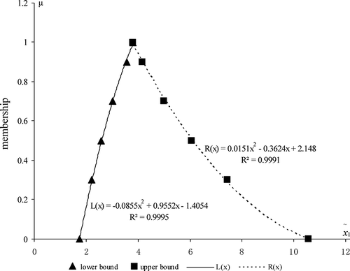
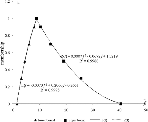
Table 1 shows the solution process for model (16). Six α-cut levels (i.e., α = 0, 0.3, 0.5, 0.7, 0.9, 1) are selected to cut the fuzzy parameters, leading to six corresponding ILP submodels. The ILP submodel under α = 0 would be solved firstly through the interactive algorithm proposed by Huang et al. (1992). Then, the ILP submodel under α = 0.3 is developed and solved based on solutions obtained through the ILP submodel under α = 0, as shown in Table 1; step by step, ILP submodels under α = 0.5, 0.7, 0.9, and 1 are obtained and solved based on interval solutions under α = 0.3, 0.5, 0.7, and 0.9, respectively. Consequently, interval solutions for model (16) under each α-cut level can be acquired. For example, when α = 0, the interval solution of would have a very wide range (= [1.75, 10.57]); however, as the value of α increases, the range of deceases (i.e., = [2.22, 7.45], = [2.59, 6.06], = [3.03, 4.99], = [3.56, 4.16]). When α = 1, model (16) becomes a deterministic model. Similar characteristics exist in the objective function (as shown in Table 1). Moreover, the GFLP model can also be supposed as an experiment, with α-cut levels are its inputs (i.e., independent variables) and the lower and upper bounds of decision variables and objective function are its outputs (i.e., dependent variables). Consequently, we can obtain six groups of samples based on the six α-cut levels. For example, the outputs for the lower bound are {1.75, 2.22, 2.59, 3.03, 3.56, 3.8}, when corresponding to the input samples {0, 0.3, 0.5, 0.7, 0.9, 1}; then we can obtained a regression function between dependent variable and independent variable α, which is considered as the L ⁻¹(x) for ; finally we would acquire the left shape function L(x) for , as shown in Figure 1. Similarly, we can obtain the right shape function for , and the left and right shape functions for the objective value . As shown in Figures 1 and 2, satisfactory curves can be acquired through polynomial statistical regression and all values of R ² are approximately equal to 1, indicating that the regression line well fits the data. Therefore, from these fitting curves, the values for , , and at any α-cut level within [0, 1] can be obtained.

Figure 1. Fuzzy membership function curve for .

Table 1. Solution process for model (17)

α	ILP Models	Solutions
0	Max = [2.5, 4]− [2, 3. 5] Subject to [0. 5, 1.4]+ [1, 2]≤ [4, 7] [0. 5, 1. 5]− [0. 5, 1. 5] ≤ [2.2, 4] ≥ 0, ≥ 0	= [1.75, 10.57] = 0.86 = [1.38, 40.57]
0.3	Max = [2.65, 3.7]− [2.3, 3.35] Subject to[0.65, 1.28] + [1.12, 1.82] ≤ [4.3, 6.4] [0.65, 1.35] − [0.65, 1.35] ≤ [2.44, 3.7] ,	= [2.22, 7.45] = 0.86 = [3.01, 25.58]
0.5	Max = [2.75, 3.5] − [2.5, 3.25] Subject to[0.75, 1.2]+ [1.2, 1.7] ≤ [4.5, 6][0.75, 1.25] − [0.75, 1.25]≤ [2.6, 3.5] ,	= [2.59, 6.06] = 0.86 = [4.35, 19.06]
0.7	Max = [2.85, 3.3] − [2.7, 3.15] Subject to[0.85, 1.12]+ [1.28, 1.58] ≤ [4.7, 5.6][0.85, 1.15]− [0.85, 1.15]≤ [2.76, 3.3] ,	= [3.03, 4.99] = 0.86 = [5.95, 14.17]
0.9	Max = [2.95, 3.1]− [2.9, 3.05] Subject to[0.95, 1.04]+ [1.36, 1.46] ≤ [4.9, 5.2][0.95, 1.05] − [0.95, 1.05]≤ [2.92, 3.1] ,	= [3.56, 4.16] = 0.86 = [7.88, 10.39]
1	Max = 3− 3 Subject to+ 1.4≤ 5 − ≤ 3 ,	= 3.8 = 0.86 = 8.83

Figure 2. Fuzzy membership function curve for the objective function

Through model (16), it is indicated that the proposed GFLP model can effectively deal with fuzzy uncertainty in both objective and constraints, and also obtain solutions expressed as fuzzy sets. The stepwise interactive algorithm (SIA) can allow fuzzy uncertainty to be communicated into solution process and would not lead to complicated intermediate submodels. Moreover, only a few of α-cut levels are needed to cut the optimization model, and consequently would not generate amounts of submodels. Therefore, the SIA would significantly reduce computation requirement. This is much meaningful for the GFLP method to be applied to practical environmental problems such as air pollution control planning.

Application To Air Quality Management

Background

For a regional system, air pollution problems are usually characterized by many emission sources at different scales, causing adverse impacts on receptors. Large sources (e.g., power plants and industrial sources) can pose a series of threats on the surrounding communities, especially under stable meteorological conditions that cause portions of the plumes to reach the ground with high concentrations. Consequently, air quality management scheme is desired for reducing air pollutant emissions through different control techniques to satisfy ambient air quality standard. In an air quality management system, many factors are involved, including pollutant generation rates, cost and treatment efficiencies of different pollutant abatement techniques, and related environmental standards such as loading capacities in different receptor zones. Establishment of a practical air quality management system is implemented through (Xu et al., 2010): (i) system investigation and data collection related to emission sources, climatic conditions, and available control measures; (ii) determination for allowable levels of pollutant emissions and environmental loading capacities; (iii) development of optimization model to minimize the total treatment cost under consideration of relevant emission standards and environmental capacities being met; and (iv) provision of emission control alternatives for decision makers to make best trade-off between system cost and excessive risk of loading capacities in different receptor zones.

In the real world, atmosphere can be polluted by many kinds of substances, such as sulfur oxides, nitrogen oxides, volatile hydrocarbons, and so on. Among them, sulfur dioxide (SO₂) is one of the most important causes for many environmental problems, such as acid rain, corrosion of buildings and monuments, and respiratory illness for human. There are amounts of sulfur dioxide emitted into atmosphere from both developed and developing countries. In the United States, more than 14 million tons SO₂ were emitted into atmosphere in 2005 even after conducting the acid rain program since 1990. And also, it was predicted that more than 30% monitors would violate the low target NAAQS (National Ambient Air Quality Standard) level in 2020 (EPA, 2009). In developing countries, the SO₂ pollution is much more serious due to rapid development of economy. For example, from 2000 to 2006, SO₂ emissions in China increased by 53%, from 21.7 to 33.2 million tons, at an annual growth rate of 7.3% (Lu et al., 2010). Therefore, formulation of desired plans for SO₂-emission control is much critical for (Li et al., 2006) (1) satisfying the environmental requirement, (2) improving the ambient air quality, (3) minimizing the required SO₂-emission control costs, and (4) identifying effective management policies.

Meanwhile, many uncertainties may be involved in a variety of impact factors and pollution-related process of a practical air quality management problem. For example, the parameters of modeling pollutant transport in the atmosphere, which are influenced by meteorological and topographical conditions, may be estimated as fuzzy sets by experts due to insufficient data; the SO₂ generation rate varied with the operating process and applied fuel could also show fuzzy features; also, environmental loading capacity for SO₂ at a given receptor location can be quantified as a fuzzy set. Simply ignoring these uncertainties in SO₂ control planning is considered undesired as it may result in inferior or wrong decisions. Therefore, identification of such uncertainties is a critical task for allocating the produced SO₂ stream to different abatement facilities with minimized economic cost and maximized environmental efficiencies.

Overview of the study system

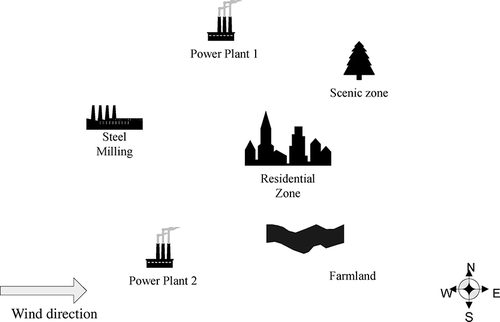
In this study, an air quality management case, proposed by Li et al., (2010), will be applied to illustrate the application of the proposed GFLP approach. As shown in Figure 3, Three SO₂ emission sources are considered in the proposed case, including two coal-fired power plants (i = 1, 2), and one steel milling factory (i = 3). The planning horizon is divided into three 5-year periods. Three land-use types (including one farmland [p = 1], one residential [p = 2], and one scenic zone [p = 3]) are considered within the studied region that adversely affected by the emitted SO₂ from three sources. According to related literatures and reports (Kitto, 1996; Li et al., 2010) three types of control measures are available for each emission source, including soda ash scrubber (SAS; j = 1), wet limestone scrubber (WLS; j = 2), and lime dry scrubber (LDS; j = 3).

Figure 3. The study system.

The objective of an air quality management model is to control adverse effects on health and property caused by air pollution. These effects are directly related to the pollutant concentration that people and property contacting. However, the air pollution emissions from different sources are presented as decision variables in the air quality management model. Consequently, it is quite desired to establish the relationship between air pollution emissions and loading concentrations. In this paper, the Gaussian dispersion model is applied to quantify the SO₂ concentrations at different receptor zones under the assumption of a cone emission plume. The ground concentration at each arbitrary downwind location (x, y) can be estimated as follows (Haith, 1982):

(17)

where C(x, y) is ground-level pollutant concentration (mg/m³) at point (x, y); x is the downwind distance from source; Q denotes pollutant emission rate (mg/sec); u is average wind velocity (m/sec) along x direction; and σ _y and σ _z represent horizontal and vertical dispersion coefficients of plume versus downwind distance x from the pollution source, and function of both meterologic conditions and downwind distance. Generally, the σ _y and σ _z can be approximated by the following equations (Davidson, 1990):

(18)

where γ₁ and β₁ are constants along y direction; γ₂ and β₂ are the coefficient along z direction, respectively. The values of γ₁, β₁, γ₂, and β₂ are related to atmospheric stability classes defined for different meteorological situations, through wind speed and solar radiation (during the day) and cloud cover during the night (Haith, 1982; Pasquill, 1974). Then, a transfer factor t_ip can be determined fromeq (17), and expressed as follows (Haith, 1982):

(19)

where t_ip represents contribution of pollutant emission rate at source i to the ground concentration of receptor zone p; the index i indicates the air pollution source; the index p indicates different receptors influenced by air pollution emissions; H_i indicates the effective height for air pollution plume from source i.

Formulation of GFLP model for air quality management

The problem under consideration focuses on mitigation of SO₂ emissions from multiple sources through different control measures over a 15-year planning horizon (divided into three periods), with a minimized system performance cost. The decision variables represent the amount of SO₂ allocated to control measure j for reduction from source i in period k, denoted as X_ijk . The objective is to minimize the total cost for SO₂ abatement. Thus, the optimization model of a regional air quality management model can be formulated as (Li et al., 2010):

(20a)

Subject to

(20b)

(20c)

(20d)

(20e)

(20f)

where i is SO₂ emission source, i = 1 and 2 represent power plants 1 and 2, respectively, i = 3 represents the steel milling factory; j is the type of SO₂ control method ( j = 1, 2, and 3 denotes SAS, WLS, and LDS, respectively); k is the planning period; X_ijk is the amount of SO₂ allocated to control measure j for reduction from source i in period k (t/day); TC _jk is the operating cost of control measure j during period k ($/t); L_k denotes the length of period k; FC _ijk is the maximum mitigation capacity of measure j at source i in period k; S_ik is the SO₂ generation amount of emission source i in period k; η _j is the efficiency of control measure j; e_ik denotes the SO₂-emission allowance for source i during period k (t/day); t_ip is the transfer factor from emission source i to receptor zone p; θ_kp is the environmental loading capacity of receptor zone p during period k (mg/m³).

In practical problem, many system parameters related to SO₂ mitigation such as cost coefficients, treatment capacities, emission allowances, and loading concentration standards may not be determined as crisp values. Many of them are estimated by experts, which are usually presented as fuzzy numbers. Moreover, solutions for decision variables expressed as fuzzy sets are also much valuable, which can provide the fluctuating ranges with related possibilities. Thus, the GFLP method is much desired to tackle fuzzy parameters and generate fuzzy solutions for this study. Therefore, model (20) can be reformulated into a GFLP model as follows:

(21a)

Subject to

(21b)

(21c)

(21d)

(21e)

(21f)

where all the parameters in model (21) are presented as fuzzy numbers. In this case, the parameters of , , , , , and are assumed to be estimated as triangular fuzzy numbers. The triangular form is the simplest type of fuzzy sets that can be easily defined, through lower-bound, upper-bound, and the most possible value of a fuzzy set. Table 2 shows the related technical and economic data including SO₂-emission rates, SO₂-emission allowances, regular costs of different pollution control measures, and allowable SO₂-loading levels for different receptors. Table 3 shows the efficiencies and capacities of different control measures. Table 4 provides the transfer factors from different sources to different receptors. These representative cost and technical data were investigated based on governmental reports and the related literatures (Environment Canada, 2009; EPA, 2004; Flagan and Seinfeld, 1988; Kitto, 1996; Li et al., 2006; Li et al., 2010; Liu et al., 2003; Nevers, 2000; Wark et al., 1998).

Table 2. Technical and economic data

	Planning Period
	k = 1	k = 2	k = 3
SO2-emission rate, (tonne/day)
Power plant 1	(240, 20, 30)	(275, 25, 35)	(310, 30, 25)
Power plant 2	(150, 18, 22)	(180, 20, 25)	(220, 25, 30)
Steel mill factory	(70, 15, 15)	(100, 20, 20)	(120, 20, 30)
SO2-emission allowance,(tonne/day)
Power plant 1	(40, 5, 5)	(38, 5, 5)	(36, 5, 5)
Power plant 2	(30, 5, 5)	(28, 5, 5)	(26, 5, 5)
Steel mill factory	(20, 5, 5)	(18, 5, 5)	(16, 5, 5)
Regular cost of different pollution control measures ($/tonne)
SAS	(76.7, 10, 10)	(84.5, 10, 10)	(97.2, 10, 10)
WLS	(59.0, 10, 10)	(65.0, 10, 10)	(74.8, 10, 10)
LDS	(38.4, 6, 6)	(42.3, 6, 6)	(48.6, 6, 6)
Allowable SO2-loading level, (mg/m^3 )(×10^−2)
Farmland zone	(22.2, 2.5, 2.5)	(20.5, 2.5, 2.5)	(18.3, 2.5, 2.5)
Residential zone	(20, 2, 2)	(19, 1.5, 1.5)	(17, 1.5, 1.5)
Scenic zone	(18, 1.2, 1.2)	(16, 1, 1)	(14, 1.5, 1.5)

Table 3. SO₂ treatment efficient and capacities

	SAS	WLS	LDS
SO2-treatment efficiency, (%)
	(0.95, 0.03, 0.03)	(0.93, 0.03, 0.03)	(0.89, 0.04, 0.04)
SO2-treatment capacity,
Power plant 1	(280, 30, 30)	(220, 20, 20)	(160, 20, 20)
Power plant 2	(180, 20, 20)	(140, 15, 15)	(100, 10, 10)
Steel milling factory	(100, 10, 10)	(100, 10, 10)	(80, 10, 10)

Table 4. The transfer factor from different sources to different receptors (× 10^{−1 1} day/m³)

	t ip
	Farmland	Residential	Scenic
Power plant 1	0.05	0.14	0.26
Power plant 2	0.11	0.16	0.04
Steel milling factory	0.13	0.31	0.15

Results and Discussion

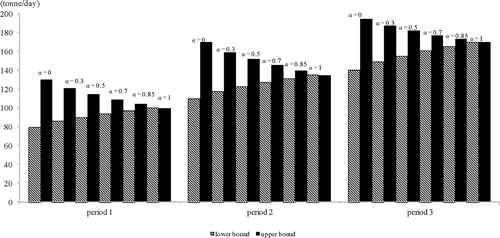
In this study, six α-cut levels (0, 0.3, 0.5, 0.7, 0.85, and 1) were considered. For each α-cut level, the fuzzy parameters can be expressed as intervals, and thus model (21) can be converted into an interval linear programming model. Table 5 presents the solutions obtained from the GFLP model for SO₂ emission abatement under each α-cut level. It shows that allocation to lime dry scrubber (LDS) would be assigned first and then to wet limestone scrubbing (WLS). This is because LDS can control SO₂-emission with a lowest operation cost among three proposed techniques; therefore, this measure is the first choice to mitigate SO₂-emission to satisfy the ambient air quality standard. The amount of SO₂ allocated to different control measures would be varied due to the temporal and spatial variations of air quality management conditions over the planning horizon. Moreover, a fuzzy interval under each α-cut level denotes a subset that the membership degree (also named degree of plausibility) of any element in the subset belonging to the original fuzzy set is larger than α. The results indicate that different α-cut levels correspond to different SO₂ allocation schedules and costs. Under a lower degree of plausibility (i.e., lower α-cut level), the intervals are wider; conversely, a higher degree of plausibility would lead to narrower intervals.

Table 5. Solutions for the GFLP under each α-cut level

	α-Cut Level
SO2 Amount	0	0.3	0.5	0.7	0.85	1
	0	0	0	0	0	0
	[80, 130]	[86, 121]	[90, 115]	[94, 109]	[97, 104.5]	100
	140	140	140	140	140	140
	0	0	0	0	0	0
	[110, 170]	[117.5, 159.5]	[122.5, 152.5]	[127.5, 145.5]	[131.25, 140.25]	135
	140	140	140	140	140	140
	0	0	0	0	0	0
	[140, 195]	[149, 187.5]	[155, 182.5]	[161, 177.5]	[165.5, 173.75]	170
	140	140	140	140	140	140
	0	0	0	0	0	0
	[42, 82]	[47.4, 75.4]	[51, 71]	[54.6, 66.6]	[57.3, 63.3]	60
	90	90	90	90	90	90
	0	0	0	0	0	0
	[70, 115]	[76, 107.5]	[80, 102.5]	[84, 97.5]	[87, 93.75]	90
	90	90	90	90	90	90
	[0, 35]	[0, 26]	[0, 20]	[0, 14]	[1.25, 9.5]	5
	[105, 125]	[112.5, 125]	[117.5, 125]	[122.5, 125]	125	125
	90	90	90	90	90	90
	0	0	0	0	0	0
	[0, 15]	[0, 10.5]	[0, 7.5]	[0, 4.5]	[0, 2.25]	0
	[55, 70]	[59, 70]	[62, 70]	[65, 70]	[67.75, 70]	70
	0	0	0	0	0	0
	[10, 50]	[16, 44]	[20, 40]	[24, 36]	[27, 33]	30
	70	70	70	70	70	70
	0	0	0	0	0	0
	[30, 80]	[36, 71]	[40, 65]	[44,59]	[47, 54.5]	50
	70	70	70	70	70	70
(×10^8)	[1.23, 2.24]	[1.35, 2.06]	[1.43, 1.94]	[1.52, 1.83]	[1.59, 1.74]	1.66

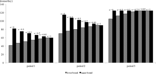
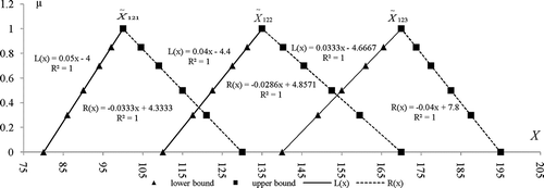
For power plant 1, all SO₂ emissions from it would be treated by lime dry scrubber (LDS) and wet limestone scrubbing (WLS) over the planning horizon. Furthermore, the LDS is the first choice for control its SO₂ emissions, which would always reach its maximum capacity (i.e., 140 t/day) in the three periods under all α-cut levels. Then the remaining emissions would be controlled by WLS, as showed in Table 5. However, the amount of SO₂ emissions allocated to WLS would vary due to the variation of SO₂ emissions from source 1under different α-cut levels. For example, when all possible values of the parameters are considered (i.e., α = 0), the allocation to WLS in period 1 is [80, 130] t/day, meaning that the lower bound flowing to WLS under α = 0 is 80 t/day, and the upper bound is 130 t/day. Furthermore, as the degree of plausibility for all the parameters increases (i.e., α-cut levels reach higher values), the solutions for SO₂ allocation to WLS would fluctuate in narrower ranges with higher lower-bound values and lower upper-bound values (e.g., [86, 121], [90, 115], [94, 109], and [97, 104.5] t/day for α = 0.3, 0.5, 0.7, and 0.85, respectively). Also, the value of 100 t/day of SO₂ emissions would be controlled by WLS under α =1, meaning that the most possible assignment of SO₂ emissions from source 1 allocated to WLS would be 100 t/day. Similar results can be obtained for SO₂ emissions from source 1 in the other two periods. However, there exist some increases for the amounts of SO₂ emissions allocated to WLS due to a rising tendency of SO₂ emissions from source 1 over the planning horizon, as shown in Figure 4. Finally, the membership functions for the SO₂-emission allocated to WLS from source 1 can be generated through linear regression, as presented in Figure 5. The R ² values are all equal to 1. Consequently, the detailed allocations can be obtained from these membership curves under every α-cut level.

Figure 4. The amount of SO₂ generated from source 1 allocated to WLS under each α-cut level.

Figure 5. The membership functions fitted for amount of SO₂ generated from source 1 allocated to WLS.

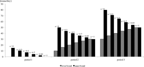
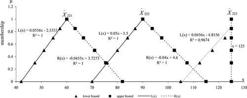
For power plant 2, the SO₂ emissions would be allocated to LDS firstly because of its lowest operation cost. The amount of SO₂ emissions flowing to LDS would be 90 t/day under every α-cut level over the planning horizon. Then the remaining emissions would be distributed to WLS after satisfying the capacity of LDS. In the first period, the SO₂-emission control condition for source 2 would be similar to that for source 1. LDS and WLS would be used to satisfy the ambient air quality standard. The widest fluctuating range for SO₂ allocated to WLS would be [42, 82] t/day in period 1 under α = 0. This range would decrease as the plausibility of the parameters increases. For example, the amounts of SO₂ distributed to WLS in period 1 would be [47.4, 75.4], [51, 71], [54.6, 66.6], and [57.3, 63.3] t/day under α = 0.3, 0.5, 0.7, and 0.85, respectively. Under α = 1, the most possible value of SO₂ allocated to WLS can be obtained (i.e., 60 t/day) in period 1. Figure 6 presents the amount of SO₂ flowing to WLS over the planning horizon. It is indicated that more SO₂ would be controlled by WLS due to the increase of SO₂ emissions from source 2. Besides, some SO₂ would be allocated to SAS (with [0, 35] t/day as the widest fluctuating range, and 5 t/day as the most possible amount) due to the capacity limitations of the LDS and WLS. Figure 7 shows the membership functions for the SO₂ emissions allocated to WLS from source 2. It is indicated that these membership curves are well fitted through linear regression (R ² = 1, 1, and 0.9674 for , and , respectively). Therefore, the detailed allocation to WLS from source 2 can be obtained under every α-cut level.

Figure 6. The amount of SO₂ generated from source 2 allocated to WLS under each α-cut level.

Figure 7. The membership functions fitted for amount of SO₂ generated from source 2 allocated to WLS.

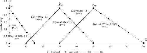
For the steel milling factory (emission source 3), most of SO₂ emissions would flow to LDS with some residuals allocated to WLS ([0, 15] t/day under α = 0, and 0 under α = 1) in period 1, as presented in Table 5. With the increase of SO₂ emissions from source 3, more allocations would be assigned to WLS (with [10, 50] and [30, 80] t/day as fluctuating ranges, and 30 and 50 t/day as the most possible values in periods 2 and 3, respectively), as shown in Figure 8. Figure 9 also presents the membership functions for SO₂ emissions allocated to WLS from steel milling factory, which can be used for generating SO₂ allocation to WLS under every α-cut level.

Figure 8. The amount of SO₂ generated from source 3 allocated to WLS under each α-cut level.

Figure 9. The membership functions fitted for amount of SO₂ generated from source 3 allocated to WLS.

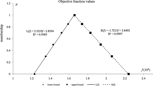
Generally, the above results indicate that, through the proposed modeling approach, uncertainties presented as fuzzy sets in all parameters can be communicated into the GFLP solution process. Table 5 also provides the total system cost from the GFLP model under six selected α-cut levels. The results suggest that different plausibility degrees of uncertain inputs would lead to varied objective function values. The lower-bound cost corresponds to advantageous conditions, while the upper-bound one is associated with more demanding conditions. For example, when α = 0, the system cost would be $[1.23, 2.24] × 10⁸. Under α = 0.3, the lower bound of system cost would be $1.35 × 10⁸ and the upper bound is $2.06 × 10⁸, meaning that the system cost would vary within $[1.35, 2.06] × 10⁷ when the plausibility of fuzzy input parameters is larger than 0.3. The objective function value of $1.66 × 10⁸ under α = 1 means that, when all fuzzy inputs reach their most possible or mean values, the system cost would be $1.66 × 10⁸. Figure 10 presents the membership curve for the total cost as fitted through linear regression. This curve coincides with the actual membership function of the total cost due to their high R ² values (R ² = 0.9985 for the left shape function, and R ² = 0.9997 for right one). Therefore, the system cost can be acquired through the fitted membership function under every plausibility degree of fuzzy inputs.

Figure 10. The membership function fitted for the total cost.

The conventional interval linear programming (ILP) method would consider uncertain parameters with known lower and upper bounds, and neglect the distributional information between the lower and upper bounds of the parameters. In this study, the solution of the GFLP model under α = 0 is identical to the solution of the conventional ILP model. As shown in Table 5, the solutions of ILP model can only provide fluctuating ranges of the decision variables without considering the plausibilities of the inputs. Consequently, ILP would generate much wide intervals for decision variables than GFLP when the distribution information is available. GFLP cannot only provide intervals for all possible decision alternatives (i.e., lower and upper bounds), but also offer plausibility degrees of the interval solutions as well as the most possible values of the decision variables and objective function value (i.e., solutions under α = 1).

Conclusions

In this study, a generalized fuzzy linear programming (GFLP) method has been developed for regional air quality management under uncertainty. The developed GFLP can deal with uncertainties expressed as fuzzy sets that exist in the constraints' left and right sides and the objective function. A stepwise interactive algorithm (SIA) was then advanced to solve GFLP model and generate solutions expressed as fuzzy sets. The SIA is implemented through (i) discretizing the membership grade of fuzzy parameters into a finite number of α-cut levels; (ii) converting the GFLP model into an interval linear programming (ILP) submodel under every α-cut level; (iii) solving the ILP submodel through an interactive algorithm and obtaining interval solutions; (iv) acquiring the membership functions of the fuzzy solutions through statistical regression method. GFLP allows uncertainties to be directly communicated into the optimization process, and has a relatively low computational requirement. This characteristic is meaningful for its applications to practical environmental management problems.

To demonstrate the applicability of the GFLP method, a regional sulfur dioxide (SO₂) control planning model was proposed to mitigate SO₂-emission from multiple sources through different control measures with a minimized system performance cost. Six α-cut levels were selected to cut the GFLP model. Interval solutions representing SO₂ allocation to different control measures from different sources were obtained under each α-cut level, and then the membership functions of the decision variables and objective were fitted through statistical regression. Compared with the conventional interval-parameter linear programming (ILP) approach, the solutions obtained through GFLP were expressed as fuzzy sets. These solutions can not only provide the fluctuating intervals for the decision variables and objective function, but also generate related plausibility degrees of these intervals. Therefore, the decision makers can make a tradeoff between model stability and the plausibility based on solutions obtained through GFLP. High plausibilities lead to narrow fluctuating ranges of decision variables and objective values, and thus result into less stability of the planning system, whereas low plausibilities produce large adjusting intervals for decision variables and objective function values and then enhance the stability of the planning system.

The developed GFLP can deal with various fuzzy set with known membership functions, regardless whether or not these functions are linear. However, it has difficulties in dealing with other kinds of uncertainties expressed as intervals and random variables. Therefore, GFLP can be further integrated with interval programming and stochastic programming methods to advance its capabilities of dealing with uncertainties expressed in multiple formats.

Acknowledgments

This research was supported by the Major Science and Technology Program for Water Pollution Control and Treatment (2009ZX07104-004) of China. The authors are grateful to the editors and the anonymous reviewers for their insightful comments and suggestions.

References

- Ammar , E.E . 2008 . On solutions of fuzzy random multiobjective quadratic programming with applications in portfolio problem . Inform. Sci. , 178 : 468 – 484 .
- Buckley , J. and Feuring , T. 2000 . Evolutionary algorithm solution to fuzzy problems: fuzzy linear programming . Fuzzy Sets Syst. , 109 : 35 – 53 .
- Chanas , S . 1983 . The use of parametric programming in fuzzy linear programming . Fuzzy Sets Syst. , 11 : 243 – 251 .
- Davidson , G.A . 1990 . A modified power law representation of the pasquuill-gifford dispersion coefficients . J. Air Waste Manage. Assoc. , 40 : 1146 – 1147 .
- Delgado , M. , Herrera , F. , Verdegay , J.L. and Vila , M.A. 1993 . Post-optimality analysis on the membership functions of a fuzzy linear programming problems . Fuzzy Sets Syst. , 53 ( 289–297 )
- Delgado , M. , Verdegay , J.L. and Vila , M.A. 1989 . A general model for fuzzy linear programming . Fuzzy Sets Syst. , 29 : 21 – 29 .
- Dubois , D. and Prade , H. 1980 . Fuzzy Sets and Systems: Theory and Applications , Academic Press : London .
- Ellis , J.H. , McBean , E.A. and Farquhar , G.J. 1985 . Chance-constrained stochastic linear programming model for acid rain abatement—I. Complete colinearity and noncolinearity . Atmos. Environ. , 19 : 925 – 937 .
- Ellis , J.H. , McBean , E.A. and Farquhar , G.J. 1986 . Chance-constrained stochastic linear programming model for acid rain abatement—II. Limited colinearity . Atmos. Environ. , 20 : 501 – 511 .
- Environment Canada . 2009 . Canada-United States Air Quality Agreement: Progress Report 2008 , Environment Canada : Ottawa, Ontario .
- Fan , Y.R. , Huang , G.H. , Li , Y.P. , Cao , M.F. and Cheng , G.H. 2009 . A fuzzy linear programming approach for municipal solid-waste management under uncertainty . Eng. Optimiz. , 41 : 1081 – 1101 .
- Flagan , R.C. and Seinfeld , J.H. 1988 . Fundamental of Air Pollution Engineering , Prentice-Hall : Englewood Cliffs, NJ .
- Guldman , J.-M . 1988 . Chance-constrained dynamic model of air quality management . Fuzzy Sets Syst. , 114 : 1116 – 1126 .
- Haith , A.D. 1982 . Environmental Systems Optimization , John Wiley & Sons : New York .
- Huang , G.H. , Baetz , B.W. and Patry , G.G. 1992 . A grey linear programming approach for municipal solid waste management planning under uncertainty . Civil Eng. Environ. Syst. , 9 : 319 – 335 .
- Kaufmann , A. and Cupta , M. 1988 . Fuzzy Mathematical Models in Engineering and Many Science , Amsterdam : North Holland .
- Kitto, J.B.1996. Air Pollution Control for Industrial Boiler Systems. Presented to ABMA Industrial Boiler Systems Conference, West Palm Beach, FL, November 6–7, 1996
- Kwon , J. , Choi , J. and Tran , T. 2007 . Emissions constrained multi-criteria-best generation mix using fuzzy dynamic programming . Int. J. Innov. Comput. Inform. Control , 3 : 41 – 52 .
- León , T. and Vercher , E. 2004 . Solving a class of fuzzy linear programs by using semi-infinite programming techniques . Fuzzy Sets Syst. , 146 : 235 – 252 .
- Li , Y.P. , Huang , G.H. , Guo , P. , Yang , Z.F. and Nie , S.L. 2010 . A dual-interval vertex analysis method and its application to environmental decision making under uncertainty . Eur. J. Oper. Res. , 200 : 536 – 550 .
- Li , Y.P. , Huang , G.H. , Veawab , A. , Nie , X.H. and Liu , L. 2006 . Two-stage fuzzy-stochastic robust programming: a hybrid model for regional air quality management . J. Air Waste Manage. Assoc. , 56 : 1070 – 1082 .
- Liu , L. , Huang , G.H. , Liu , Y. , Fuller , G.A. and Zeng , G.M. 2003 . A fuzzy-stochastic robust programming model for regional air quality management under uncertainty . Engineer. Optimiz. , 35 : 177 – 199 .
- Lu , H.W. , Huang , G.H. and He , L.A. 2010 . Two-phase optimization model based on inexact air dispersion simulation for regional air quality control . Water Air Soil Pollut. , 211 : 121 – 134 . doi: 10.1007/s11270-009-0286–3
- Lu , H.W. , Huang , G.H. , Liu , L. and He , L. 2008 . An interval-parameter fuzzy-stochastic programming approach for air quality management under uncertainty . Environ. Eng. Sci. , 25 : 895 – 909 .
- Lu , Z. , Streets , D.G. , Zhang , Q. , Wang , S. , Carmichael , G.R. , Cheng , Y.F. , Wei , C. , Chin , M. , Diehl , T. and Tan , Q. 2010 . Sulfur dioxide emissions in china and sulfur trends in east asia since 2000 . Atmos. Chem. Phys. , 10 : 6311 – 6331 .
- Lv , Y. , Huang , G.H. , Li , Y.P. , Yang , Z.F. and Li , C.H. 2009 . Interval-based air quality index optimization model for regional environmental management under uncertainty . Environ. Eng. Sci. , 26 : 1585 – 1597 .
- Nevers , D.N. 2000 . Air Pollution Control Engineering , 2nd , McGraw-Hill : New York .
- Nie , X.H. , Huang , G.H. , Li , Y.P. and Liu , L. 2007 . IFRP: A hybrid interval-parameter fuzzy robust programming approach for waste management planning under uncertainty . J. Environ. Manage. , 84 : 1 – 11 .
- Pasquill , F. 1974 . Atmospheric Diffusion: The Dispersion of Windborne Material from Industrial and Other Sources , Halsted Press : New York .
- Qin , X.S. , Huang , G.H. and Liu , L.A. 2010 . Genetic-algorithm-aided stochastic optimization model for regional air quality management under uncertainty . J Air Waste Manage. Assoc. , 60 : 63 – 71 . doi: 10.3155/1047-3289.60.1.63
- Rommelfanger , H . 1996 . Fuzzy linear programming and applications . Eur. J. Oper. Res. , 92 : 512 – 527 .
- U.S. Environmental Protection Agency (EPA) . 2004 . SO2 Allowance Market Analysis: 2004 Update , U.S. EPA : Washington, DC .
- U.S. Environmental Protection Agency (EPA) . 2009 . Proposed Revisions to Sulfur Dioxide Primary National Air Quality Standard , Washington, DC : U.S. EPA .
- Wark , K. , Warner , C.F. and Davis , W.T. 1998 . Air Pollution: Its Origion and Control , 3rd , Harper Collins Publishers : New York .
- Xu , Y. , Huang , G.H. , Qin , X.S. and Huang , Y. 2010 . An inexact fuzzy-chance-constrained air quality management model . J. Air Waste Manage. Assoc. , 60 : 805 – 819 . doi: 10.3155-1047-3289.60.7.805
- Zadeh , L.A . 1965 . Fuzzy sets . Inform Control , 8 : 338 – 353 .