Switching nonparametric regression models

Abstract

We propose a methodology to analyse data arising from a curve that, over its domain, switches among J states. We consider a sequence of response variables, where each response y depends on a covariate x according to an unobserved state z. The states form a stochastic process and their possible values are j=1, … , J. If z equals j the expected response of y is one of J unknown smooth functions evaluated at x. We call this model a switching nonparametric regression model. We develop an Expectation–Maximisation algorithm to estimate the parameters of the latent state process and the functions corresponding to the J states. We also obtain standard errors for the parameter estimates of the state process. We conduct simulation studies to analyse the frequentist properties of our estimates. We also apply the proposed methodology to the well-known motorcycle dataset treating the data as coming from more than one simulated accident run with unobserved run labels.

Keywords:

• nonparametric regression
• machine learning
• mixture of Gaussian processes
• latent variables
• EM algorithm
• motorcycle data

AMS Subject Classification:

• Primary: 62G08, 62G05
• Secondary: 62M99

1. Introduction

In this paper we propose a methodology to analyse data arising from a curve that, over its domain, switches among J states. The state at any particular point is determined by a latent process, which also determines a function.

Suppose we have a sequence of response variables, , where y_i depends on a covariate x_i (usually time) according to an unobserved state z_i, also called a hidden or latent state. The possible values of the states are j=1, … , J. If z_i=j the expected response of y_i is f_j(x_i). We call this model a switching nonparametric regression model.

The objective of the proposed methodology is to estimate the f_js as well as to estimate the regression error variance and the parameters governing the distribution of the state process. We also obtain standard errors (SEs) for the proposed parameter estimators of the state process. We consider two types of hidden states, those that are independent and identically distributed (iid) and those that follow a Markov structure. The Markov structure would usually require x to be time.

As an application we consider a new type of analysis of the well-known motorcycle dataset. The data consist of 133 measurements of head acceleration taken through time in a simulated motorcycle accident (see Figure 1). A table containing the raw data can be found in Härdle (1990) and the data are also available in the software R. Analyses appearing in the literature treat the data as coming from one simulated accident (see, for instance, Silverman 1985; Härdle and Marron 1995; Rasmussen and Ghahramani 2002; Gijbels and Goderniaux 2004; Wood 2011; Yang and Ma 2011; Lázaro-Gredilla, Van Vaerenbergh, and Lawrence 2012; Schiegg, Neumann, and Kersting 2012). However, close examination of the data suggests the measurements are from J>1 accidents. Indeed, although Schiegg et al. fit a mixture of three Gaussian processes (or experts) they write ‘the experts of the mixture of Gaussian processes have no specific meaning’. In the discussion of Silverman (1985) Prof. A.C. Atkinson wrote ‘inspection of [the Figure], particularly in the region 30–40 ms, suggests that the data may not be a single time series but are rather the superposition of, perhaps, three series’. Professor Silverman replied ‘Professor Atkinson is right about the motorcycle data in that they are the superposition of measurements made by several instruments but the data I have presented are precisely in the form they were made available to me’. The details of the dataset will most likely remain unclear as the original report (Schmidt, Mattern, and Schüler 1981) seems to be no longer available.

Figure 1. Motorcycle data. Head acceleration in g (one g ≈ 9.8 m/s²) versus the time in milliseconds after impact.

The motorcycle data should be analysed as coming from J>1 simulated accident runs with hidden (lost) run labels. We carry out just such an analysis, recovering and estimating the functions corresponding to each of the accident runs, using the following device: we treat the data as arising from one curve that switches among J>1 functions with hidden function labels. We choose J using an ad hoc Akaike information criterion (AIC). To our knowledge this is the first time that the motorcycle data are analysed taking into account that they describe more than one simulated accident.

The paper is organised as follows. In Section 2 we present an overview of the proposed methodology. A literature review on the topic is presented in Section 3. In Section 4 we describe the solution for the estimation problem. The SEs for the parameter estimators of the state process are calculated in Section 5. In Section 6 we present the results of simulation studies. An application of the proposed methodology to the motorcycle data is shown in Section 7. Some discussion is presented in Section 8.

The methodology is implemented in R via the package switchnpreg. This package is available on CRAN (http://cran.r-project.org/).

2. Overview of the proposed methodology

Suppose we have observed data x_i, y_i, and hidden states z_i, i=1, … , n. The states form a stochastic process and their possible values are j=1, … , J. Given z_i, , for independent with mean of zero and variance of one. Therefore, given the f_js and the z_is, the y_is are independent with the mean of y_i equal to and the variance equal to .

Let , and . Define γ to be the set of parameters defining the distribution of given and the s. So, for instance, if the ε_is are normally distributed, then . Let α be the vector of parameters that determine the joint distribution of . If the z_is are iid, then the parameter vector α is of length J with jth component equal to P(z_i=j). If the z_is follow a Markov structure, the parameter vector α consists of initial and transition probabilities.

Our goal is to estimate , along with SEs or some measure of accuracy of estimates of the parameters in α.

To obtain the parameter estimates we maximise

(1)

where the exact form of is chosen by the user. We consider two forms of arising from two approaches, a frequentist approach called penalised log-likelihood estimation and a Bayesian approach where the posterior density is maximised. These two approaches are computationally similar and consist of using the Expectation–Maximisation (EM) algorithm (Dempster, Laird, and Rubin 1977) to maximise Equation (1).

In the frequentist approach we assume that f_j″ exists almost everywhere and for j=1, … , J and maximise Equation (1) with

The λ_js are the smoothing parameters.

If one were to take a Bayesian approach, one would elicit a prior distribution for the parameters in θ. For the f_js, we consider a Gaussian process regression approach (Rasmussen and Williams 2006) with independent and f_j a Gaussian process with mean function and covariance function, , that depends on a vector of parameters λ_j. We place a non-informative prior on the other parameters. Therefore, we can write where is an n×n matrix with entries given by with known. In our applications and simulations we assume the following covariance function

(2)

with parameter vector . These parameters control the amount of smoothness of each curve f_j and, as in the penalised log-likelihood approach, are called smoothing parameters.

No matter how the penalty P arises in Equation (1), whether via a Bayesian or a penalised log-likelihood approach, we choose the values of the λ_js automatically by cross-validation.

3. Background

Similar models have appeared in the machine learning literature, where they are called mixture of Gaussian processes models (Tresp 2001; Rasmussen and Ghahramani 2002; Ou and Martin 2008). A main difference between our model and the model in these three papers is in the distribution of the z_is. All three papers begin by assuming that the z_is are independent, conditional on the parameters governing the latent process. In Rasmussen and Ghahramani and in Ou and Martin, the process parameters are , j≥1, which are modelled using a Dirichlet distribution. Rasmussen and Ghahramani use a limit of a Dirichlet distribution in order to model an infinite number of possible hidden states, to avoid choosing the number of states. Ou and Martin use a finite number of states to avoid computational complexity. Both papers use an ad hoc modification of the distribution of the z_is to allow z_i to depend on x_i in a smooth way; see Rasmussen and Ghahramani's equation (5) and Ou and Martin's equation (13). However, as remarked by Rasmussen and Ghahramani in the discussion, the properties of the resulting joint distribution of the z_is are not completely known. Tresp's distributional assumptions are more straightforward: he assumes that the distribution of z_i depends on x_i according to a logit model governed by a Gaussian process. None of these papers consider Markov z_is.

While the three papers contain methodology that can, in principle, lead to estimation of the f_js and the latent variable process parameters, the papers focus on estimation of just one function – the mixture. Thus the resulting methodology is a form of variable bandwidth smoothing (see, for instance, Fan and Gijbels 1992). In contrast, our goal is estimation of the individual processes that make up the mixture and estimation of the parameters governing the hidden state process, along with SEs. We see the distinction between the goals by considering the analysis of the motorcycle data: Rasmussen and Ghahramani present just one function to summarise the data. We present J>1 functions, one for each of the J simulated accidents, and we estimate the expected proportion of data points from each function, and provide SEs. We also conduct extensive simulation studies of the frequentist properties of the estimates.

A closely related approach, used in density estimation, is the Gaussian mixture model, where the ith data point comes from one of a finite set of Gaussian distributions, determined by the value of a latent variable z_i. In his work on Gaussian mixture models, Bilmes (1998) considered two types of latent variables: in the first the latent variables are independent and identically distributed and in the second they follow a Markov structure. The latter corresponds to a classic hidden Markov model, which is the same as our approach for Markov zs if the f_js are constant.

These models are not to be confused with the work of Shi, Murray-Smith, and Titterington (2005) on Gaussian process mixtures for regression and Chiou (2012) on functional mixture prediction. These authors analyse data from M independent curves where the entire ith curve is a realisation of one of J Gaussian processes, determined by the value of the latent variable z_i. In contrast, like Tresp, Rasmussen and Ghahramani, and Ou and Martin, we consider M=1 observed curve, which switches among J Gaussian processes.

We see that the literature contains many similar but distinct models with names containing the words Gaussian and mixture. For this reason, we prefer to call our models and those of Tresp (2001), Rasmussen and Ghahramani (2002) and Ou and Martin (2008) switching nonparametric regression models as we feel this is more descriptive. To our knowledge, no one has considered a Markov structure for the latent variables to estimate multiple functions, nor has anyone used the non-Bayesian penalised likelihood approach. Our frequentist approach and our calculation of SEs appear to be new.

4. Parameter estimation via the EM algorithm

We use the EM algorithm to obtain the parameter estimates for the penalised log-likelihood and Bayesian approaches. The E-step of the algorithm is exactly the same for both approaches. The M-step differs only in the part involving the calculation of fˆ_j. In the M-step we restrict our calculations to normally distributed errors. Furthermore, for the M-step of the penalised approach, we model each f_j as a linear combination of K known cubic B-spline basis functions , that is, with the set of unknown parameters determining f_j. We justify this by the fact that, in the M-step, the maximising f_js are cubic smoothing splines (see Silverman 1985, Equation (5.1) or Heckman 2012). In our simulation studies and application we consider K=40 basis functions with equally spaced knots following the recommendations of Ruppert, Wand, and Carroll (2003). One could use automatic methods to choose K such as the ones described by Ruppert et al. (2003), based on the minimisation of a cross-validation criterion. We have not done this as using K large with penalty suffices.

Let be the log-likelihood based on the observed data. Our goal is to find θˆ that maximises

(3)

The form of is complicated, since it involves the distribution of the latent z_is. Therefore, we use an EM algorithm to maximise Equation (3). We can show (see, for instance, Cappé, Moulines, and Rydén 2005; McLachlan and Krishnan 2008) that our EM algorithm generates a sequence of estimates, θ^(c), c≥1, satisfying .

To define our EM algorithm, let be the joint distribution of the observed and latent data given θ, also called the complete data distribution. In what follows view θ as an argument of a function, not as a random variable. Note that we write to denote the conditional expected value of assuming that the data and are generated with parameter vector θ^(c).

The proposed EM algorithm consists of the following two steps based on writing , where and

(4)

1. Expectation step (E-step): calculate

2. Maximisation step (M-step): let Use the Expectation–Conditional maximisation (ECM) algorithm (Meng and Rubin 1993) to find so that . We can show that if then as desired. For details, see Cappé et al. (2005) and McLachlan and Krishnan (2008).

4.1. E-step: general z_is

Using and assuming a regression model with normal errors, we obtain

(5)

where whose exact form depends on the model for the z_is.

In the following sections we calculate and considering different models for the latent variables. Note that depends on the model for the z_is only through .

4.1.1. E-step: iid z_is

In this section we calculate and assuming that the latent variables are iid with parameter vector , where and .

Since the z_is are iid, we obtain

(6)

Note that we can easily calculate Equation (6) when the regression errors are normally distributed. To calculate for iid z_is we can write

(7)

and, therefore,

(8)

4.1.2. E-step: Markov z_is

Here we calculate and assuming a Markov structure for the latent variables , with initial probabilities , j=1, … , J. We assume that

1. the ith latent variable depends on past latent variables only via the (i−1)st latent variable, i.e. and

2. the transition probabilities do not depend on i, that is,

To compute when the z_is are Markov, we use the results of Baum, Petrie, Soules, and Weiss (1970). These authors let and and show how to calculate these recursively using what they call the forward and backward procedures, respectively. Because of the Markovian conditional independence

Thus, we can calculate via

Now let us consider . Since for Markov z_is

(9)

(10)

where . This can be expanded as which we easily calculate using the normality assumption for the regression errors.

More details on how to obtain the expressions for and can be found in Bilmes (1998), Rabiner (1989) and Cappé et al. (2005).

4.2. M-step

For the M-step we combine our discussion of iid zs and Markov zs. We want to find so that . For normally distributed errors is given by Equation (5) and, therefore, we can write

(11)

(12)

(13)

We want to maximise S as a function of with θ^(c), and thus the s, fixed. We also consider the smoothing parameters, , to be fixed. We apply a natural extension of the EM approach, the ECM algorithm, to guarantee that .

Because the expression for does not depend on the f_js or s, the f_js and s that maximise S are the f_js and s that maximise (11) + (12). Therefore, the form of the maximising f_js and s will not depend on the model for the zs. Their only dependence on the model for the zs is via the s.

Thus, to obtain the vector of parameter estimates, , we apply the ECM algorithm as follows.

1. Hold the s and the parameters in α fixed and maximise (11) plus (12) with respect to . Let

   (14)
   For the Bayesian approach this is equivalent to maximising obtaining Let be with in replaced by . For the penalised log-likelihood approach, , where is the vector of coefficients corresponding to f_j and is an n×K matrix with entries . Thus, we maximise with respect to φ_j yielding where is a K×K matrix with entries . Let be φˆ_j with in replaced by . So we let .

2. Now holding the s and the parameters in α fixed and maximising Equation (11) with respect to we get

   (15)
   Let be with f_j(x_i) replaced by . If we assume for all j, then we find that
   (16)
   We improve our variance estimates by adjusting the degrees of freedom to account for the estimation of the f_js. We do that by replacing the denominator of Equation (15) by and the denominator of Equation (16) by , where and is the so called hat matrix satisfying . For the Bayesian approach
   (17)
   and for the penalised approach
   (18)
   This modification is similar to a weighted version of what Wahba (1983) has proposed for the regular smoothing spline case.

3. Now we hold the f_j(x)s and s fixed and maximise S with respect to the parameters in α. Since Equations (11) and (12) do not depend on α, we only maximise in Equation (13). Because the form of does depend on the model for the zs, we must obtain the estimates of α for each model separately. For iid z_is, where , using Equation (8) and Lagrange multipliers with the restriction that , we obtain: For Markov z_is we first maximise given in Equation (10) with respect to the transition probabilities, the a_ljs. Holding π_j fixed and using a Lagrange multiplier with the constraint , we obtain: Maximising Equation (10) with respect to the π_js with yields: .

5. SEs for the parameter estimators of the state process

We use the results of Louis (1982) to obtain SEs for the estimators of the parameters of the state process. We consider for iid z_is J≥2 possible state values. For Markov z_is we restrict the possible number of states to J=2 to reduce complexity.

Louis (1982) derived a procedure to obtain the observed information matrix when the maximum likelihood estimates are obtained using the EM algorithm. The procedure requires the computation of the gradient and of the second derivative matrix of the log-likelihood based on the complete data and can be implemented easily within the EM steps. We use Louis's technique with known γ to derive the formula for the information matrix associated with αˆ. We then plug our final estimates, αˆ and γˆ, into this formula, yielding our estimated information matrix:

(19)

with is as in Equation (4), the gradient vector of and the associated second derivative matrix.

In the next sections we show how to calculate Î for the different models for the z_is.

5.1. SEs: iid z_is

We rewrite Equation (7) in terms of as

Consider the matrix in Equation (19) evaluated at and . Its jlth entry, for j≠l, is equal to n/pˆ_J where . Let . Then the jjth entry is

One can also show that the matrix in Equation (19) evaluated at αˆ and γˆ has off-diagonal elements jl equal to and jth diagonal element given by

5.2. SEs: Markov z_is

For Markov z_is we show how to obtain SEs for the estimates of the transition probabilities for J=2 possible state values. We apply Louis's method to find SEs for â₁₂ and â₂₁ by using in Equation (9) with π₁ and π₂ fixed.

Then the 2×2 matrix with π₁ and π₂ fixed, evaluated at , and is given by

Calculating the 2×2 matrix is straightforward but tedious, involving sums of expectations of indicator functions. The summands require the calculation of , and , with r, s, t and u taking values 1 or 2 and Δ a positive integer. These conditional probabilities can be calculated using Bayes’ Theorem and the Markovian conditional independence of the z_is.

6. Simulations

We carry out simulation studies considering that the z_is can take values 1 or 2 and they can be either iid or follow a Markov structure. The parameters of interest are estimated using both the Bayesian and the penalised log-likelihood approaches presented in Section 4. For each simulation study 300 independent datasets are generated.

6.1. Simulated data

We consider three types of simulation studies according to three different types of simulated data. Table 1 presents a summary of these simulation studies. In all studies we use the same vector of evaluation points and the same true functions f₁ and f₂. The vector consists of n=199 equally spaced points, . The true functions evaluated at , that is, the vectors and , are obtained by sampling from a multivariate normal distribution with mean of zero and covariance matrix determined by Equation (2). We let the parameter U_j in Equation (2) be equal to so that . We consider and for and , respectively.

Table 1.  Summary of the simulation studies.

Sim'n	Type of zis	zis parameters	s
1	iid	p1=0.7
		p2=0.3
2	Markov
		a12=0.3
		a21=0.4
3
		a12=0.1
		a21=0.2

In each simulation study after we obtain the commonly used and we generate each of the 300 simulated datasets as follows.

1. Generate the z_is according to the specified model (iid or Markov).

2. Generate , , where and the ε_is are independent standard normal random variables.

In our first simulation study we generate data assuming that the z_is are independent with . The top row of Figure 2 shows an example of a dataset of this type.

Figure 2. Top row: Simulation 1 (iid z_is with p₁=0.7). Bottom row: Simulation 2 (Markov z_is with a₁₂=0.3 and a₂₁=0.4). Example of simulated data along with the initial and final estimates of f₁ and f₂ obtained using the Bayesian approach and the penalised log-likelihood approaches. The light-coloured dots correspond to z=2 and the dark-coloured dots to z=1. The solid lines correspond to the true functions f₁ and f₂, respectively. The dot-dashed lines are the initial estimates of f₁ and f₂ obtained using the function estimate method. The dashed lines are the final estimates of f₁ and f₂. See online version for colours.

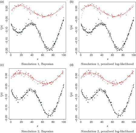
For the second and third simulation studies we consider Markov z_is. In the second study we use transition probabilities and and in the third study a₁₂=0.1 and a₂₁=0.2. For both studies we consider initial probabilities . The bottom rows of Figure 2 and Figure 3 both show examples of datasets from the second and third studies, respectively. With this Markov structure, we see that the system can stay in one state for a long time, giving information about just one of the functions during that range of x values. This is more pronounced in Figure 3 when a₁₂ and a₂₁ are small.

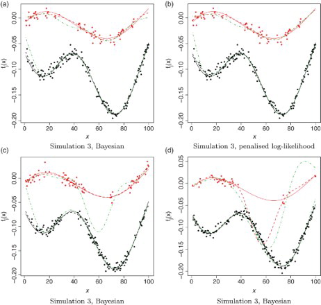
Figure 3. Simulation 3 (Markov z_is with a₁₂=0.1 and a₂₁=0.2). Top row: Example of simulated data along with the initial and final estimates of f₁ and f₂. The light-coloured dots correspond to z=2 and the dark-coloured dots to z=1. The solid lines correspond to the true functions f₁ and f₂, respectively. The dot-dashed lines are the initial estimates of f₁ and f₂ obtained using the residual-based method. The dashed lines are the final estimates of f₁ and f₂. Bottom row: Example of simulated datasets along with initial estimates (dot-dashed lines) that yield (c) good and (d) bad final function estimates (dashed lines) using the Bayesian approach. See online version for colours.

6.2. Initial values

To analyse the data via our EM algorithm, we need to provide initial values of all of the parameter estimates. We set the initial estimates of all of the parameters governing the distribution of the z_is to 0.5.

Examples of initial values of and are shown as the green lines in Figures 2 and 3. In order to automatically obtain such initial values, we first assign temporary values to the latent variables, creating two groups of observations (one consisting of all (x_i, y_i)s with temporary z_i value equal to 1, the other consisting of the remaining (x_i, y_i)s). For each group, we estimate the corresponding . For the Bayesian approach we estimate by its posterior mean, commonly used in Gaussian regression (Rasmussen and Williams 2006), with initial . For the penalised log-likelihood approach we use smoothing splines to estimate the f_js. The smoothing parameters for both approaches are chosen by cross-validation (CV). For the Bayesian approach we also add the restriction that if the λ_j obtained by CV is smaller than 10 we use a bigger value, in this case 15.

Two methods are used to assign the temporary values to the z_is.

• Function estimate method: we fit one curve, , to the whole dataset using a standard cubic smoothing spline. If , we set z_i=1, otherwise we set z_i=2.

• Residual-based method: we obtain as in the function estimate method and calculate the residuals . We then divide the evaluation interval into small subintervals. Within each subinterval, we consider all residuals corresponding to x_is within that subinterval. We use the k-means algorithm (k=2) to partition these residuals into two groups. We label the group with the smaller mean as group 1 .

The function estimate method is used in Simulations 1 and 2, but this method performs poorly for data as in Simulation 3, when the z process tends to remain in one state for an extended period, yielding information about only one of the f_js. Therefore we developed and used the residual-based method in Simulation 3. The residual-based method requires a choice of number of sub-intervals and sub-interval lengths. Our choice of sub-intervals is based on examination of results from a few datasets. The chosen sub-intervals are as follows: [1, 34], [34.5, 67.5] and [68, 100].

A wide range of reasonable initial estimates of f₁ and f₂ yields good final estimates. For all datasets considered we can always find reasonable initial estimates by eye. For most datasets the proposed automatic methods work. However, for a few datasets the automatic procedures produce obviously bad initial estimates that do not allow the method to recover. This is particularly true in Simulation 3. Figure 3(c) and 3(d) show examples of simulated datasets with initial function estimates that yield good and bad final estimates, respectively.

To obtain an initial estimate of σ² we first use the initial function estimates and the two temporary groups of observations to obtain the sample variance of the residuals of each group separately adjusting for the correct degrees of freedom. We then set the initial estimate of σ² equal to the pooled variance.

6.3. Choice of the smoothing parameters, the λ_js

We find the optimal λ_js iteratively starting with initial values , j=1, … , J. The choice of the s is important to obtain good final estimates of the f_js. We found out that very small s do not lead to good final estimates as more points tend to be initially misclassified. For the Bayesian approach, in each dataset we set the s to the values used to obtain the initial function estimates, which were forced to be greater than 10. For the penalised log-likelihood approach, we use one value of for all datasets: we set to a value that worked well when tested on a couple of simulated datasets.

We update the λ_js as follows.

1. With , j=1, … , J, use the EM algorithm of Section 4 to find the pˆ_ijs, and the fˆ_js.

2. Discard the fˆ_js from Step 1.

3. Treat and the pˆ_ijs as fixed and thus W_j as in Equation (14) as fixed. For each λ on a grid and each j=1, … , J, calculate with as in Equation (17) or Equation (18).

4. For each j=1, … , J, set as the value in the grid that minimises the following cross-validation criterion: where is the ith entry of the diagonal of .

5. Repeat 1–4 with , j=1, … , J, till convergence.

We use the final values of the λ_js to obtain all of the parameter estimates from the EM algorithm as in Step 1.

6.4. Results

Figures 2 and 3 present examples of the fitted values and (dashed lines) for all three simulation studies.

We assess the quality of the estimated functions via the pointwise empirical mean squared error (EMSE). The empirical mean squared error of fˆ_j at a given point x_i is calculated as follows: where is the estimate of f_j in the sth simulated dataset. We calculate the EMSE for both initial and final estimates of the f_js. In all three simulation studies we observe that the EMSE_j values are higher at the edges than at the middle of the evaluation interval. We also observe that in all simulation studies the final estimates produce smaller values of EMSE_j than the initial estimates, which indicates that the proposed methodology improves the initial naive estimates (see Figures 1 and 2 of the Supplementary Material).

Comparing the approaches’ EMSEs, we see that, in Simulations 1 and 2, the Bayesian approach produces slightly smaller values of EMSE_j for the final function estimates than the penalised log-likelihood approach. In Simulation 3 the Bayesian approach produces slightly smaller values of EMSE for fˆ₁ than the penalised log-likelihood approach except for the right edge. In Simulation 3, there is no clear winner for estimating f₂. In addition, both approaches produce values of EMSE for fˆ₂ that are larger than the values obtained in Simulations 1 and 2 (see Figure 4). The plots from Simulation 2 are omitted as they are similar to the ones from Simulation 1.

Figure 4. Top row: Simulation 1 (iid z_is with p₁=0.7). Bottom row: Simulation 3 (Markov z_is with a₁₂=0.1 and a₂₁=0.2). EMSE of the final estimates of f₁ and f₂ using the Bayesian (dashed lines) and the penalised log-likelihood (solid lines) approaches.

To further study the quality of our method, we look at possible cases of misclassification. Table 2 presents the number of simulated datasets with at least one value of when z_i=2. Table 3 shows the number of simulated datasets with at least one value of when z_i=1. For Simulations 1 and 2 all misclassifications occur at the edges of the evaluation interval, indicating that the proposed method sometimes has problems at the edges. The same is true in Simulation 3 for the penalised log-likelihood approach. In Simulation 3, the Bayesian approach leads to problems not just at the edges: two datasets have large values of when z_i=1 at the middle of the evaluation interval when f₁ and f₂ are closer.

Table 2.  Number of simulated datasets with at least one value of pˆ(z_i=1|y_i)>0.2 when z_i=2.

Approach	Simulation 1	Simulation 2	Simulation 3
Bayes	0^a	0^a	4
Penalised log-likelihood	0^a	0^a	1

was never larger than 0.04 when the true z_i=2.

Table 3.  Number of simulated datasets with at least one value of pˆ(z_i=2|y_i)>0.2 when z_i=1.

Approach	Simulation 1	Simulation 2	Simulation 3
Bayes	3	3	14
Penalised log-likelihood	2	1	13

Table 4 presents the mean and standard deviation of all 300 estimates of σ² for each simulation study and each approach. All estimates are obtained adjusting the degrees of freedom to account for the estimation of the f_js. We can observe that the means for the Bayesian approach are closer to the true value of σ² () than the means obtained using the penalised log-likelihood approach. The medians (not included in the table) for the Bayesian approach are also closer to than the medians for the penalised log-likelihood approach.

Table 4.  Estimates of σ² (true value=5×10⁻⁵).

Simulation	Approach	(SD)
1	Bayesian	4.984 (0.491)
	PL^b	4.912 (0.498)
2	Bayesian	4.982 (0.556)
	PL	4.916 (0.579)
3	Bayesian	4.935 (0.517)
	PL	4.880 (0.519)

^aSD, standard deviation.

^bPL, penalised log-likelihood.

Table 5 contains the mean and the standard deviation of the estimates of the parameters of the z_is for each simulation study for both approaches. Note that the standard deviations of the estimates are close to the values of the means of the proposed SEs, as desired.

Table 5.  Estimates of the parameters of the z process.

					Empirical coverage
Sim'n	z Parameters	Approach	Mean (SD^a)	Mean of SEs	90%	95%
1	p1=0.7	Bayesian	0.699 (0.032)	0.032	90.7%	95.7%
		PL^b	0.699 (0.032)	0.032	90.7%	95.7%
2	a12=0.3	Bayesian	0.300 (0.043)	0.043	90.0%	94.3%
		PL	0.300 (0.043)	0.043	90.0%	94.3%
	a21=0.4	Bayesian	0.399 (0.053)	0.053	90.3%	95.7%
		PL	0.399 (0.053)	0.053	90.3%	95.7%
3	a12=0.1	Bayesian	0.105 (0.025)	0.027	93.0%	97.3%
		PL	0.105 (0.024)	0.027	93.3%	97.3%
	a21=0.2	Bayesian	0.208 (0.052)	0.050	91.7%	92.7%
		PL	0.208 (0.052)	0.050	91.7%	92.7%

^aSD, standard deviation.

^bPL, penalised log-likelihood.

Table 5 also shows the empirical coverage percentages of both a 90% and a 95% confidence interval. We consider confidence intervals of the form: where z_α/2 is the α/2 quantile of a standard normal distribution with α=0.1 and 0.05. The empirical coverage percentages for Simulations 1 and 2 are close to the true level of the corresponding confidence interval. In Simulation 3 this is not case. In particular, some of the 90% confidence intervals for a₂₁ are based on estimates of a₂₁ that are so poor that even the 95% confidence intervals do not contain the true value of a₂₁. In this case the 95% confidence intervals have roughly the same empirical coverage as the 90% confidence intervals.

We also study the performance of our proposed methodology for a lower signal-to-noise ratio. We conduct the same three simulation studies described in Section 6.1 considering a regression error variance five times bigger, that is, . To facilitate comparisons the y_is are generated using the same z_is from the previous simulations where . We obtain results (see Supplementary Material) that are similar to the ones described in the previous paragraphs with two exceptions. The first exception is that there are more misclassified points than before, particularly at the interval where the two functions are closest. However, we notice that sometimes a misclassification can still yield good final estimates of f₁ and f₂ as shown in Figure 5 of the Supplementary Material. The second exception is that in Simulation 3 the penalised log-likelihood approach produces smaller values of empirical mean squared error for fˆ₂ than the Bayesian approach (see Figure 10(b) of the Supplementary Material).

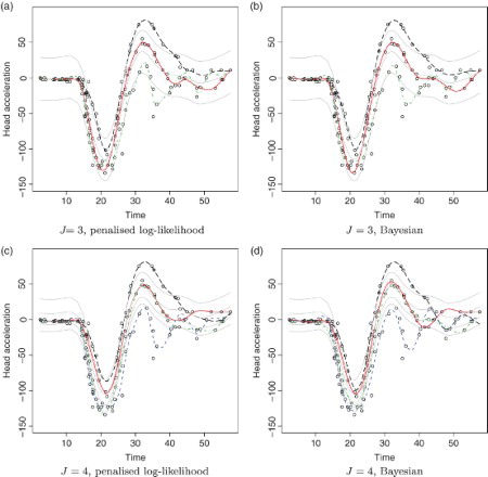
Figure 5. Motorcycle data. Top row: final function estimates obtained for J=3 using (a) the penalised log-likelihood approach and (b) the Bayesian approach. Bottom row: final function estimates obtained for J=4 using (c) the penalised log-likelihood approach and (d) the Bayesian approach. The thin light-coloured lines correspond to the initial function estimates, which are constant shifts of a smoothing spline fit to all the data. See online version for colours.

We also conduct a simulation study to investigate the performance of both Bayesian and penalised log-likelihood approaches when the true functions are deterministic smooth functions. We generate data as in Simulation 2 (see Table 1) with true functions f₁ and f₂ similar to the ones generated from the stochastic model, however each is now deterministically obtained as a linear combination of 10 cubic B-splines with knots that are a subset of the ones used in the estimation. The results (see Supplementary Material) are very similar to ones obtained in Simulation 2 with f₁ and f₂ generated from a stochastic model. Again, the Bayesian approach produces slightly smaller values of EMSE than the penalised log-likelihood approach.

In conclusion we find that the Bayesian and penalised log-likelihood approaches are comparable in terms of the EMSEs of the fˆ_js, the bias and variance of the parameter estimates and the coverage of the confidence intervals for the parameters of the z process. However, we prefer using the penalised log-likelihood approach for its computational speed.

7. Analysis of the motorcycle data

In this section we fit our proposed methodology to the motorcycle dataset treating the measurements as coming from J>1 functions (one for each simulated accident) with hidden (unknown) function labels. We fit the data assuming that the hidden states, which correspond to the unknown accident run labels, are iid. We estimate the model parameters using both the Bayesian and the penalised log-likelihood approaches. The smoothing parameters, the λ_js, are selected by cross-validation as in Section 6.3. For the Bayesian approach we set the covariance parameter U_j in Equation (2) to be known and fixed at where fˆ is a regular smoothing spline fit to the data and is the corresponding hat matrix.

The dataset contains 39 time points with multiple acceleration measurements, which our method does not currently allow. So, we jitter each of those time points by adding a small random noise.

We fit the model considering J=2, … , 6 functions, choosing J to minimise , where is the hat matrix corresponding to .

We apply the proposed model considering both equal and different regression error variances. However, the choice of J is not so obvious when we use a common regression error variance. Therefore, the results presented here are obtained considering different error variances.

For the Bayesian approach the AIC is minimum for a model with J=4 and for the penalised log-likelihood, when J=3. As both results appear sensible, we present them both (see Figure 5).

Table 6 presents the estimated model and smoothing parameters when J=3 for both the Bayesian and the penalised log-likelihood approaches. We can observe the qualitative agreement between the results. For instance, the green curve has the largest variance. The mixing proportion estimates agree, well within the reported SEs. Although the values of the λ_js are not comparable between the two approaches, we see that for both methods, the green curve has the smallest value of λ_j, indicating that the green curve is the least smooth curve.

Table 6.  Results for J=3 with corresponding fitted curves in Figure 5(a) and 5(b).

Approach	Curve		pˆj (s.e.)	λj
Penalised	Black (long-dashed)	43.054	0.269 (0.047)	0.893
Log-likelihood	Red (solid)	14.227	0.395 (0.053)	0.890
(Figure 5(a))	Green (dot-dashed)	171.048	0.337 (0.053)	0.167
Bayesian	Black (long-dashed)	50.134	0.272 (0.047)	3.901
(Figure 5(b))	Red (solid)	8.593	0.361 (0.050)	5.005
	Green (dot-dashed)	184.478	0.367 (0.052)	2.512

Table 7 is similar to Table 6 and presents the results for J=4.

Table 7.  Results for J=4 with corresponding fitted curves in Figure 5(c) and 5(d).

Approach	Curve		pˆj (s.e.)	λj
Penalised	Black (long-dashed)	50.348	0.211 (0.042)	1.591
Log-likelihood	Red (solid)	7.623	0.232 (0.050)	1.213
(Figure 5(c))	Green (dot-dashed)	7.245	0.244 (0.051)	0.825
	Blue (dashed)	135.968	0.313 (0.049)	0.545
Bayesian	Black (long-dashed)	48.376	0.223 (0.043)	3.782
(Figure 5(d))	Red (solid)	5.473	0.221 (0.045)	4.805
	Green (dot-dashed)	1.106	0.198 (0.042)	5.377
	Blue (dashed)	145.440	0.358 (0.048)	3.355

8. Discussion

In this paper we proposed a model to analyse data arising from a curve that, over its domain, switches among J states. We called this model a switching nonparametric regression model. Overall our main contributions include the introduction and development of the frequentist approach to the problem, including the calculation of SEs for the parameter estimators of the latent process and the study of the frequentist properties of the proposed estimates via simulation studies. As an application we analysed the well-known motorcycle data in an innovative way: treating the data as coming from J>1 simulated accident runs with unobserved run labels.

Supplementary data

Supplemental material for this article can be accessed at http://dx.doi.org/10.1080/10485252.2014.941364.

Acknowledgements

We would like to thank Prof Dr med Rainer Mattern for all his efforts in trying to obtain a copy of Schmidt et al. (1981), the original report containing the motorcycle data. It appears the report is no longer available. We also thank the Editor, Associate Editor and reviewers for their insightful questions and comments.

Funding

This work was supported by the National Science and Engineering Research Council of Canada.

References

- Baum, L., Petrie, T., Soules, G., and Weiss, N. (1970), ‘A Maximization Technique Occurring in the Statistical Analysis of Probabilistic Functions of Markov Chains’, The Annals of Mathematical Statistics, 41, 164–171. doi: 10.1214/aoms/1177697196
- Bilmes, J. (1998), ‘A Gentle Tutorial of the EM Algorithm and its Application to Parameter Estimation for Gaussian Mixture and Hidden Markov Models’, Technical Report TR-97-021, ICSI.
- Cappé, O., Moulines, E., and Rydén, T. (2005), Inference in Hidden Markov Models, New York: Springer Verlag.
- Chiou, J. (2012), ‘Dynamical Functional Prediction and Classification, with Application to Traffic Flow Prediction’, The Annals of Applied Statistics, 6, 1588–1614. doi: 10.1214/12-AOAS595
- Dempster, A.P., Laird, N.M., and Rubin, D.B. (1977), ‘Maximum Likelihood from Incomplete Data via the EM Algorithm’, Journal of the Royal Statistical Society Series B, 39, 1–38.
- Fan, J., and Gijbels, I. (1992), ‘Variable Bandwidth and Local Linear Regression Smoothers’, Annals of Statistics, 20, 2008–2036. doi: 10.1214/aos/1176348900
- Gijbels, I., and Goderniaux, A. (2004), ‘Bootstrap Test for Change-Points in Nonparametric Regression’, Journal of Nonparametric Statistics, 16, 591–611. doi: 10.1080/10485250310001626088
- Härdle, W. (1990), Applied Nonparametric Regression, Cambridge: Cambridge University Press.
- Härdle, W., and Marron, J. (1995), ‘Fast and Simple Scatterplot Smoothing’, Computational Statistics & Data Analysis, 20, 1–17. doi: 10.1016/0167-9473(94)00031-D
- Heckman, N. (2012), ‘Reproducing Kernel Hilbert Spaces Made Easy’, Statistics Surveys, 6, 113–141. doi: 10.1214/12-SS101
- Lázaro-Gredilla, M., Van Vaerenbergh, S., and Lawrence, N.D. (2012), ‘Overlapping Mixtures of Gaussian Processes for the Data Association Problem’, Pattern Recognition, 45, 1386–1395. doi: 10.1016/j.patcog.2011.10.004
- Louis, T. (1982), ‘Finding the Observed Information Matrix when using the EM Algorithm’, Journal of the Royal Statistical Society Series B, 44, 226–233.
- McLachlan, G., and Krishnan, T. (2008), The EM Algorithm and Extensions (2nd ed.), New York: Wiley.
- Meng, X.L., and Rubin, D.B. (1993), ‘Maximum Likelihood Estimation via the ECM Algorithm: A General Framework’, Biometrika, 80, 267–278. doi: 10.1093/biomet/80.2.267
- Ou, X., and Martin, E. (2008), ‘Batch Process Modelling with Mixtures of Gaussian Processes’, Neural Computing & Applications, 17, 471–479. doi: 10.1007/s00521-007-0144-4
- Rabiner, L. (1989), ‘A Tutorial on Hidden Markov Models and Selected Applications in Speech Recognition’, Proceedings of the IEEE, 77, 257–286. doi: 10.1109/5.18626
- Rasmussen, C., and Ghahramani, Z. (2002), ‘Infinite Mixtures of Gaussian Process Experts’, in Advances in Neural Information Processing Systems 14: Proceedings of the 2001 Conference, Vol. 2, Cambridge, MA: The MIT Press, pp. 881–888.
- Rasmussen, C.E., and Williams, C.K.I. (2006), Gaussian Processes for Machine Learning, Cambridge, MA: The MIT Press.
- Ruppert, D., Wand, M.P., and Carroll, R.J. (2003), Semiparametric Regression, Cambridge: Cambridge University Press.
- Schiegg, M., Neumann, M., and Kersting, K. (2012), ‘Markov Logic Mixtures of Gaussian Processes: Towards Machines Reading Regression Data’, in Proceedings of the 15th International Conference on Artificial Intelligence and Statistics, Vol. 22.
- Schmidt, G., Mattern, R., and Schüler, F. (1981), ‘Biomechanical Investigation to Determine Physical and Traumatological Differentiation Criteria for the Maximum Load Capacity of Head and Vertebral Column with and without Protective Helmet under the Effects of Impact’, EEC Research Program on Biomechanics of Impacts. Final report Phase III, Project G5, Institut für Rechtsmedizin, Universität Heidelberg.
- Shi, J., Murray-Smith, R., and Titterington, D. (2005), ‘Hierarchical Gaussian Process Mixtures for Regression’, Statistics and Computing, 15, 31–41. doi: 10.1007/s11222-005-4787-7
- Silverman, B. (1985), ‘Some Aspects of the Spline Smoothing Approach to Non-Parametric Regression Curve Fitting’, Journal of the Royal Statistical Society Series B, 47, 1–52.
- Tresp, V. (2001), ‘Mixtures of Gaussian Processes’, in Advances in Neural Information Processing Systems 13: Proceedings of the 2000 Conference, Cambridge, MA: The MIT Press, pp. 654–660.
- Wahba, G. (1983), ‘Bayesian “Confidence Intervals" for the Cross-Validated Smoothing Spline’, Journal of the Royal Statistical Society Series B, 45, 133–150.
- Wood, S.N. (2011), ‘Fast Stable Restricted Maximum Likelihood and Marginal Likelihood Estimation of Semiparametric Generalized Linear Models’, Journal of the Royal Statistical Society Series B, 73, 3–36. doi: 10.1111/j.1467-9868.2010.00749.x
- Yang, Y., and Ma, J. (2011), ‘An Efficient EM Approach to Parameter Learning of the Mixture of Gaussian Processes’, in Proceedings of the 8th International Conference on Advances in Neural Networks, Berlin: Springer-Verlag, pp. 165–174.