Generalized linear mixed-model (GLMM) trees: A flexible decision-tree method for multilevel and longitudinal data

Abstract

Objective: Decision-tree methods are machine-learning methods which provide results that are relatively easy to interpret and apply by human decision makers. The resulting decision trees show how baseline patient characteristics can be combined to predict treatment outcomes for individual patients, for example. This paper introduces GLMM trees, a decision-tree method for multilevel and longitudinal data.

Method: To illustrate, we apply GLMM trees to a dataset of 3,256 young people (mean age 11.33, 48% girls) receiving treatment at one of several mental-health service providers in the UK. Two treatment outcomes (mental-health difficulties scores corrected for baseline) were regressed on 18 demographic, case and severity characteristics at baseline. We compared the performance of GLMM trees with that of traditional GLMMs and random forests.

Results: GLMM trees yielded modest predictive accuracy, with cross-validated multiple R values of .18 and .25. Predictive accuracy did not differ significantly from that of traditional GLMMs and random forests, while GLMM trees required evaluation of a lower number of variables.

Conclusion: GLMM trees provide a useful data-analytic tool for clinical prediction problems. The supplemental material provides a tutorial for replicating the GLMM tree analyses in R.

Keywords:

• multilevel data
• decision making
• decision-tree methods
• mixed-effects models
• subgroup detection

Clinical or methodological significance: Decision tree-methods provide results that may be easier to apply in clinical practice than traditional statistical methods, like the generalized linear mixed-effects model (GLMM).

• GLMM trees provides a flexible decision-tree algorithm that can be applied to a wide range of research questions in psychotherapy research, and that can account for multilevel and longitudinal data structures.

• Using a large patient-level dataset on outcomes at UK mental health services, we show that GLMM trees provide accuracy on par with traditional GLMMs and random forests, a modern machine-learning method, while requiring less information for making a prediction.

• The supplementary material provides a manual which shows researchers how they can fit GLMM trees to their own data in the open-source statistical programming environment R.

Introduction

Many empirical research questions in mental health are focused on decision making in clinical practice. For example: Which patients are (not) at risk for a recurrent disorder? Which patients will benefit most (least) from treatment? Such research questions are traditionally addressed using additive linear models, like the generalized linear model (GLM) or the generalized linear mixed-effects model (GLMM). For example, in recent publications in Psychiatry Research, GL(M)Ms were applied by O’Keeffe et al. (2018) to predict dropout among adolescents receiving psychotherapy, and by Koffmann (2020) to predict outcomes among adults receiving psychotherapy. Although such GL(M)Ms allow for identifying predictors associated with psychotherapy outcomes, they do not directly show what to do in clinical decision making. For example, if the predictor variable is continuous, where should we draw the line for deciding high versus low risk? And when some risk factors are present, but others absent, how should we combine the risk factors into a single decision?

In contrast to traditional GL(M)Ms, recursive partitioning or decision-tree methods do show what to do in decision making. Instead of describing the association between predictor and outcome variables by a mathematical formula (e.g., $\hat{y}=b_0+b_1{x}_1+b_2{x}_2+b_3{x}_3$), recursive partitioning methods describe the association between predictor and outcome variables by a binary decision tree. Such decision trees are easier to apply in clinical practice, where information, time and computational power are limited and costly (e.g., Gigerenzer, Todd, & the ABC Research Group, 1999). This relative ease of interpretation and application has led several authors of earlier studies published in Psychotherapy Research to apply decision-tree methods for predicting treatment outcomes (e.g., Berman & Hegel, 2014; Hannöver et al., 2002; Hannöver & Kordy, 2005; Hansen et al., 2007). An additional advantage of decision-tree methods is their non-parametric nature: They do not require assumptions like linear associations or normally distributed residuals, and allow for specifying a large number of potential predictor variables, which may even exceed the number of observations.

The current paper aims to introduce a recent decision-tree method that allows for the analysis of multilevel and longitudinal datasets: GLMM trees (Fokkema et al., 2018). Such data structures are commonly encountered in psychotherapy research, and GLMM trees may thus provide a useful data-analytic tool in such studies. The paper is structured as follows: In the remainder of the Introduction, we discuss the position of decision trees within the broader area of machine learning. Next, we discuss the building blocks of the GLMM tree algorithm. In the Method and Results section, we illustrate how the GLMM tree algorithm can provide a clinically useful alternative to traditional GLMMs. We apply the GLMM tree algorithm to an existing dataset from an earlier study on patient-level predictors of young people’s treatment outcomes in UK mental-health services (Edbrooke-Childs et al., 2017). We compare the resulting decision trees in terms of predictive accuracy and interpretability with the traditional GLMMs originally fitted to the data. We also compare the performance with that of random forests, a machine-learning algorithm which has often been found to rank highest in terms of predictive accuracy. In the Discussion section, we integrate our results with earlier findings on (mixed-effects) decision-tree methods. For readers interested in fitting GLMM trees to their own data, the supplementary material provides a tutorial on how to fit GLMM trees in the statistical programming environment R (R Core Team, 2020).

Decision Trees and Machine-learning Methods

Compared to other machine-learning algorithms for prediction, the main advantage of single decision trees is their interpretability: the tree-like structure is preeminently suited for practical decision making. At the same time, however, the tree-like structure is relatively simple, so it may provide only a coarse approximation of very smooth or fine-grained associations possibly present in a dataset. As a result, single decision trees generally do not rank among the most accurate machine-learning methods (e.g., Fernández-Delgado et al., 2014; Gacto et al., 2019; Zhang et al., 2017).

To improve the predictive accuracy of single decision trees, so-called ensembling techniques can be used. For example, techniques like bagging (Breiman, 1996), boosting (Schapire & Freund, 1995) and random forests (Breiman, 2001) grow a large number of trees on random samples of the original dataset. This allows the predictive model to flexibly approximate the associations present in a dataset in a smooth manner. As a result, these ensemble methods provide better predictive accuracy, exceeding that of any of the individual trees (e.g., Rokach, 2010). The main disadvantage of such tree ensembles is their complexity: instead of a single decision tree, the predictive model now consists of a large number (generally ≥ 500), that can no longer be visually grasped.

This high predictive accuracy as well as high complexity is shared by other state-of-the-art machine learning methods, like support vector machines and artificial neural networks. Studies comparing the predictive performance of machine-learning methods on a wide range of data problems generally find decision-tree ensembles, support vector machines, and sometimes artificial neural networks to rank highest in terms of predictive accuracy. For example, Gacto et al. (2019) found random forests and support vector machines to rank highest in solving non-linear regression problems. Zhang et al. (2017) found boosted tree ensembles matched or exceeded the predictive performance of support vector machines and random forests. Fernández-Delgado et al. (2014) found random forests to provide highest predictive performance, followed by support vector machines, neural networks and boosted tree ensembles.

The increase in predictive accuracy provided by methods like support vector machines, neural networks and decision-tree ensembles, however, comes at the cost of complexity. How these methods compute predictions from the values of predictor variables is difficult, if not impossible, for humans to grasp. Several explanatory methods have therefore been proposed, which aim to explain how complex statistical methods arrive at their predictions (e.g., Lundberg & Lee, 2017; Ribeiro et al., 2016). However, these methods currently suffer from several drawbacks. As noted by Carvalho et al. (2019), there is no consensus on how to measure the quality of these explanations. Thus, there is no guarantee that the explanations provide enough detail to understand what the black-box method is doing (Rudin, 2019). Rudin (2019) also noted that black-box predictive models combined with (similarly complex) explanatory methods may yield complicated decision pathways that increase the likelihood of human error. This was corroborated by Kaur et al. (2020), who experimentally studied the use of explanatory methods among data scientists; they found that the explanations were often over-trusted and few users were able to accurately describe what the visualizations were showing.

At the same time, a recent systematic review found no performance benefit of machine learning over logistic regression for clinical prediction models (Jie et al., 2019), indicating that the trade-off between higher accuracy and lower complexity may not always hold. A possible explanation for this finding is that even for flexible models, in order to capture complex patterns, these patterns need to be observed repeatedly. This may require very large sample sizes, especially for the prediction of human behaviour and life outcomes, which have been noted to be difficult to predict (e.g., Salganik et al., 2020). Earlier, Hand (2006) already noted that the gains in predictive performance offered by more complex methods over simpler ones are generally small, and that practical, real-world characteristics of prediction problems may render such differences irrelevant.

Thus, whether for individual prediction problems a method with state-of-the-art predictive accuracy should be preferred over a simpler method likely depends on several characteristics of the data problem, such as the relative gain in predictive performance, the amount and cost of information required for making a prediction, the extent to which the training data is a random sample from the target population, and/or the quality of the data (e.g., measurement error, mislabeled cases). Especially in situations where the gain in predictive accuracy offered by more complex methods is small, or where collecting and processing of information is costly, simpler methods like decision trees or regularized GLMs may be preferred.

Unbiased Recursive Partitioning and Extension to Multilevel and Longitudinal Data

The GLMM tree algorithm is an extension of the unbiased recursive partitioning framework of Hothorn et al. (2006) and Zeileis et al. (2008). Unbiased here means that the methods do not present with a variable selection bias, in which variables with a larger number of categories or unique values are more likely to be selected for partitioning, even if they are no more informative than their competitors (e.g., White & Liu, 1994). Several of the earlier recursive partitioning methods, like the Classification and Regression Trees algorithm (CART; Breiman et al., 1984), suffer from such a variable selection bias. The aforementioned studies published in Psychotherapy Research also employed the CART algorithm, or adjusted versions thereof. More recent recursive partitioning algorithms, like the classification tree algorithm of Kim and Loh (2001), the conditional inference tree algorithm of Hothorn et al. (2006), and the model-based recursive partitioning algorithm of Zeileis et al. (2008) do not suffer from this variable selection bias.

These algorithms mitigate variable selection bias by separating variable and cut-point selection: in every node, the splitting variable is selected first, based on test statistics quantifying the association between predictor and response variables. At each step, the variable with the lowest p value of the association test is selected for splitting. After selection of the splitting variable, the cut-point or splitting value is selected through optimizing the sum of the loss function in the two resulting nodes. The use of statistical tests for selection of splitting variables also provides a stopping rule: When none of the potential predictor variables in the current node has a p value below the pre-specified α level, splitting is halted.

The GLMM tree algorithm is based on the GLM tree algorithm, a specific case of the model-based recursive partitioning algorithm of Zeileis et al. (2008). GLM trees fit a recursive partition based on a (generalized) linear model: The nodes in a GLM tree consist of subgroup-specific GLMs, which contain an intercept term and possibly the effects of one or more predictor variables. The subgroups are described in terms of additional covariates: variables that are used to define the partition or subgroups, which are not included as predictors of the GLM.

The GLMM tree algorithm extends the GLM tree algorithm by accounting for possible dependence between observations in longitudinal or multilevel datasets. In such datasets, individual observations are nested in higher-level units: In multilevel datasets, individual observations (e.g., patients) may be nested within higher-level units (e.g., therapists and/or treatment centres), while in longitudinal datasets, measurements obtained at different occasions may be nested within patients. Traditionally, such datasets are analyzed with GLMM-type linear models, which account for the correlated nature of observations through the estimation of random effects. In (generalized) linear models, this has been found to yield more accurate standard errors and lower type-I and -II errors (e.g., Moerbeek, 2004; Steenbergen & Jones, 2002; Van den Noortgate et al., 2005). Only recently have decision-tree methods been developed that allow for the analysis of such correlated data structures. Accounting for correlated structures in decision-tree analyses has been shown to yield more accurate, as well as less complex trees (e.g., Fokkema et al., 2018; Hajjem et al., 2017; Sela & Simonoff, 2012). Further technical detail on the estimation of GLMM trees is provided in Fokkema et al. (2018).

GLMM trees allow for the analysis of a wide range of research questions. First, outcome variables may be continuous, binary, or counts; predictor variables may be continuous or (ordered) categorical. Second, in addition to finding predictors of (clinical) outcomes, GLMM trees can also be used to find moderators in the association between predictor and outcome variables in multilevel and longitudinal datasets. Examples of particular relevance to psychotherapy research include the detection of moderators of treatment effect, where the interest is in detecting subgroups which show differential effects for two or more treatments (Doove et al., 2014; Fokkema et al., 2018; Seibold et al., 2016). Another example is the detection of subgroups in growth curve models, where the interest is in finding subgroups with different initial levels of symptomatology or different patterns of change over time. As such, GLMM trees provide a flexible statistical tool for informing a wide range of clinical decision questions. In the current paper, we focus on a relatively simple prediction problem, where the value of treatment outcomes are predicted using a range of baseline patient characteristics, while possible differences due to service providers are accounted for. Although GLMM trees can be applied to more complex research questions, the aim of this paper is to provide an introductory primer on the use of a GLMM trees. Readers interested in more complex analyses can consult Fokkema et al. (2018) and/or the examples in the documentation of package glmertree (Zeileis & Fokkema, 2019), that can be used for fitting GLMM trees.

It should be noted that there are other algorithms and software packages that allow for recursive partitioning of GLMM-type models, such as SEM trees (Brandmaier et al., 2013), longRpart (Abdolell et al., 2002) and longRpart2 (Stegmann et al., 2018). In the current paper, we focus on GLMM trees, because it allows for partitioning based on variables measured at both the lowest level (e.g., patient level) as well as higher levels (e.g., therapist, treatment centre, region level). The other packages mentioned allow for partitioning based on variables measured at the highest level only, which precludes analyses such as the one in the current paper, where we want to detect subgroups with different treatment outcomes based on patient-level characteristics (level I), while accounting for treatment outcome differences between treatment centres (level II).

Method

Dataset

Edbrooke-Childs et al. (2017) analyzed a sample of 3,256 young people who received treatment at one of 13 mental-health service providers in the UK. The analyses were performed on complete cases. Summary statistics for age, gender and ethnicity are provided in Table I. Potential predictor variables were demographic variables (age, gender, ethnicity), case characteristics (coding the presence or absence of several mental and behavioural disorders), and severity characteristics (measures of impairment in functioning) assessed at baseline.

Table I. Descriptive statistics of the full sample (N = 3,256).

		M (SD) or %	Min	Max
Age		11.33 (3.42)	4.00	18.00
Gender	Female	48%
Ethnicity	White	69%
	Mixed	5%
	Asian	8%
	Black or Black British	6%
	Other	5%
	Not reported or missing	13%
Case characteristics	Hyperactivity	10%
	Emotional problems	55%
	Conduct problems	20%
	Eating disorder	5%
	Self-harm	8%
	Autism	9%
	Special education needs	8%
	Other presenting problems	22%
	Infrequent characteristics	12%
Total difficulties T1		18.49 (7.13)	0.00	39.00
Total difficulties T2		15.48 (7.87)	0.00	38.00
Unadjusted treatment outcome		0.00 (1.00)	−4.51	5.12
Adjusted treatment outcome		0.16 (1.21)	−6.44	5.86

Specifically, ethnicity was captured using the categories from the 2001 Census from the UK Office for National Statistics, and grouped for analysis according to the levels reported in Table I. Case characteristics included absence/presence of hyperactivity, emotional problems, conduct problems, eating disorder, self-harm, autism, special education needs and other presenting problems (Table I). Furthermore, the presence of case characteristics occurring with a frequency of <5% in the sample were grouped into a single “infrequent characteristics” indicator (i.e., psychosis, intellectual disability, developmental disorder, habit disorder, substance misuse, child protection concerns, and Child Act order in place). Severity characteristics were assessed using the impact supplement of the Strengths and Difficulties Questionnaire (SDQ; Goodman, 1997). This yielded six indicators for the severity of mental-health problems: duration (rated on a 5-point scale ranging from absent to > 1 year), overall distress, and impairment on home life, friendships, classroom performance, and leisure activities (all rated on a 3-point scale ranging from little or no severity to high severity).

Treatment outcome was quantified as the total mental-health difficulties score on the SDQ, assessed approximately 4–8 months after the first (baseline) assessment. This score was computed by summing the four difficulties subscales of the SDQ (conduct problems, emotional problems, peer problems, hyperactivity; descriptive statistics presented in Table I). Two outcome variables were calculated: An unadjusted treatment outcome, which is the standardized value of the total difficulties score corrected for the baseline assessment, with higher values indicating poorer outcomes. Secondly, an adjusted treatment outcome was calculated, which corresponds to the so-called “added value score” on the SDQ¹ (Ford et al., 2009). It reflects the standardized difference between observed and expected change in mental health difficulties, and aims to correct for spontaneous improvement and regression to the mean. It can be interpreted as an effect size, where positive values indicate more improvement and negative values indicate more deterioration than expected. We analyzed both treatment outcomes, because the unadjusted outcome can be interpreted as a weighted change score, while the adjusted outcome can be interpreted as deterioration compared to what would have been expected, had the young person not accessed services.

Statistical Analyses

All analyses were performed in the statistical programming environment R (R Core Team, 2020). Mixed-effects regression models were fitted using package lme4 (Bates et al., 2015). A random intercept was estimated with respect to mental-health service provider and restricted maximum likelihood (REML) estimation was employed. GLMM trees were fitted using package glmertree (Zeileis & Fokkema, 2019). Again, a random intercept was estimated with respect to mental-health service provider. Default settings were employed: REML was employed for estimation of the fixed- and random-effects parameters, an α level of .05 was employed and p values for the variable selection tests were Bonferroni corrected. Random forests were fitted using package randomForest (Liaw & Wiener, 2002). We included the indicator for mental-health service provider as a categorical predictor variable. Furthermore, earlier studies have found good predictive performance for the standard random forest algorithm in multilevel data when the intra-class correlation was small (Hajjem et al., 2014; Karpievitch et al., 2009; Martin, 2015). Because this was also the case in our study, we employed default settings: no a-priori restrictions on tree size were applied, 500 bootstrap samples were drawn, and for selecting each split, a random sample of 1/3 of the potential predictor variables was used.

To estimate the models’ predictive accuracies, we employed 10-fold cross validation. Cross validation provides a more realistic estimate of generalization error than calculating variance explained in the training sample (Hastie et al., 2009). Cross-validated predictions for the mixed-effects regression and GLMM tree models were computed based on both random and fixed effects, so that predictions for all fitted models captured the effect of mental-health service provider. Prediction error was quantified as the mean squared difference between predicted and observed response variable values (MSE). The standard error of the MSE was computed as the standard deviation of the squared difference between predicted and observed response variable values, divided by the square root of the sample size. Furthermore, we standardized MSE values through dividing by the sample standard deviations of the response variables. This yields a measure which can be interpreted as the multiple R coefficient. In the current study, this multiple R value may seem relatively low, compared to values that readers are used to, because it was computed based on cross-validation instead of training data and because the treatment outcome variables were computed so that they already accounted for baseline SDQ values.

Results

In the original analyses of Edbrooke-Childs et al. (2017), linear mixed-effects models were fitted to predict treatment outcomes, in which fixed effects were estimated for the demographic, case and severity characteristics, and a random intercept was estimated with respect to service provider. This yielded seven statistically significant predictors of treatment outcome (Table II), and estimated intra-class correlations of 0.05–0.07. We applied the GLMM tree algorithm to the same data and research question. As in the original analyses, demographic, case and severity characteristics were included as potential predictor variables (see Table I), and a random intercept was estimated with respect to service provider.

Table II. Statistically significant predictors of treatment outcome according to the original analyses of Edbrooke-Childs et al. (2017).

Unadjusted treatment outcome	Adjusted treatment outcome
Age	Autism
Ethnicity	Infrequent case characteristics
Eating disorder	Disorder duration
Hyperactivity
Autism
Infrequent case characteristics

The GLMM tree for the unadjusted treatment outcome is presented in Figure 1. Higher values of the unadjusted treatment outcome reflect poorer treatment outcomes. Age at referral was selected as the first predictor variable, with poorer average treatment outcome for those aged ≤ 9.1, compared to those aged > 9.1 at referral. In the lower age group, presence of emotional problems was selected as the second predictor variable, with the absence of emotional problems yielding poorer treatment outcomes, on average. In the group with emotional problems, gender was selected as a predictor variable: boys had poorer treatment outcomes than girls, on average. In the group with higher age at referral (age at referral > 9.1), the presence of an autistic disorder was selected as a second predictor variable: those with an autistic disorder had poorer treatment outcomes, on average.

Figure 1. GLMM tree for the unadjusted treatment outcome. Higher values represent poorer treatment outcomes. Panels depict subgroup sizes (N) and estimated fixed-effects means (M) with standard errors (SE). Note that SEs account for random variability between treatment centres, but not for the searching of the tree structure.

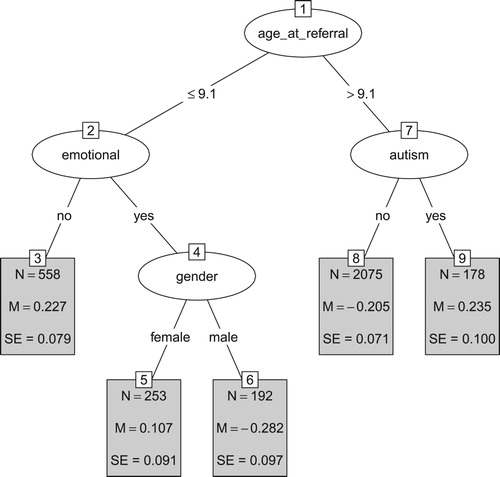
The terminal nodes in Figure 1 also present standard errors for the estimated subgroup means. These standard errors are computed based on a confirmatory mixed-effects model, which accounts for variability between treatment centres, but not for the searching of the tree structure. Thus, they provide a useful indication of variability, but may underestimate true variability. Taking into account the standard errors, we can conclude that the unadjusted treatment outcomes do not differ significantly between nodes 3 and 5, between nodes 3 and 9, between nodes 5 and 9, between nodes 6 and 8.

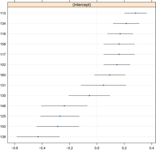
The predicted values of the random intercept are depicted in Figure 2, which indicates a quite symmetric distribution around the mean of 0. The estimated intra-class correlation was 0.06. Poorest outcomes were observed for service provider 113, and best outcomes were observed for service provider 138. Note that the error bars in Figure 2 do not account for the searching of the tree structure and may therefore be too small.

Figure 2. Random-effects predictions of the GLMM tree for the unadjusted treatment outcome. The y-axis represents indicators for service provider. The x-axis represents the predicted value of the random intercept, where higher values represent poorer treatment outcomes. Blue dots represent point predictions, black lines represent point predictions ±1.96 times the standard error. Note that these standard errors do not account for the searching of the tree structure.

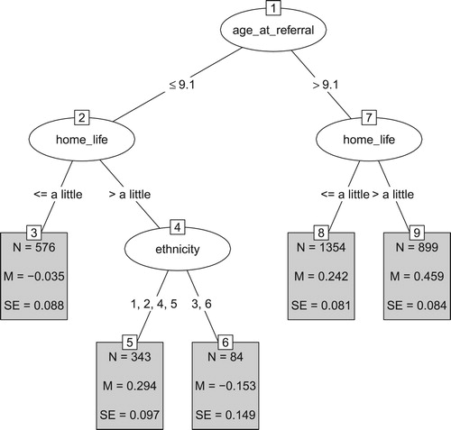
The GLMM tree for the adjusted treatment outcome is presented in Figure 3. Lower values of the adjusted treatment outcome reflect poorer outcomes. Again, we see that that lower age at referral is associated with poorer treatment outcomes. In both age groups, the next split was based on the parent-reported impairment of mental-health problems on home life, with stronger impairment on home life yielding better outcomes (than would be expected based on baseline SDQ mental-health difficulty scores). In the group aged ≤ 9.1 at referral, a third split was created based on ethnicity, with Asian and non-reported or missing ethnicity yielding better treatment outcomes, compared to other ethnicity groups. This split should be interpreted with care: The two resulting subgroups (especially terminal node six) are rather small, yielding less reliable estimates of the difference between the two groups, which is also evidenced by the relatively large standard errors. Furthermore, the split was partly based on ethnicity being not reported or missing, making it difficult to draw conclusions on the meaning of this split. Taking into account the standard errors reported in the terminal nodes, we can conclude that the adjusted treatment outcomes do not differ significantly between nodes 3 and 6, between nodes 5 and 8, and between nodes 5 and 9.

Figure 3. GLMM tree for the adjusted treatment outcome. Lower values reflect poorer treatment outcomes. Panels depict subgroups sizes (N), estimated fixed-effects means (M) and their respective standard errors (SE). Ethnicity was coded White (1), Mixed (2), Asian (3), Black or Black British (4), Other (5), Not reported or missing (6). Note that SEs account for random variability between treatment centres, but not for the searching of the tree structure.

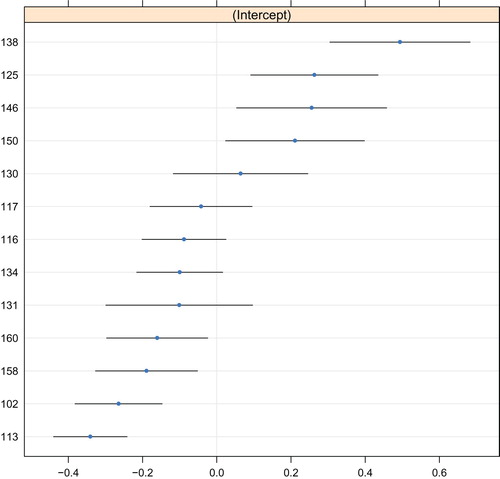
The predicted values of the random intercept are depicted in Figure 4, which indicates a rather symmetric distribution around the mean of 0. The intra-class correlation was 0.05. Again, poorest outcomes were observed for service provider 113, and best outcomes were observed for service provider 138.

Figure 4. Random-effects predictions of the GLMM tree for the adjusted treatment outcome. The y-axis represents indicators for service provider. The x-axis represents the predicted value of the random intercept, where lower values represent poorer treatment outcomes. Blue dots represent point predictions, black lines represent point predictions ±1.96 times the standard error. Note that these standard errors do not account for the searching of the tree structure.

We compared predictive accuracy of GLMM trees with that of traditional GLMMs and random forests using 10-fold cross validation. Results are presented in Table III, which shows that GLMM trees yielded accuracy on par with that of the traditional GLMMs and the random forests. The traditional GLMMs yielded slightly higher predictive accuracy than GLMM trees. Random forests yielded somewhat lower predictive accuracy than both traditional GLMMs and GLMM trees. Taking into account the standard errors of the MSEs indicates that predictive accuracy did not differ significantly between methods.

Table III. Prediction error of GLMM trees, traditional GLMMs and random forests, estimated through 10-fold cross validation.

	Unadjusted treatment outcome		Adjusted treatment outcome
Method	R	MSE (se)	R	MSE (se)
GLMM tree	.252	0.931 (0.028)	.179	1.421 (0.043)
Traditional GLMM	.253	0.930 (0.027)	.205	1.406 (0.043)
Random forest	.195	0.956 (0.028)	.049	1.464 (0.044)

Note. MSE denotes mean squared error; se denotes standard error; R is the square root of the treatment outcome variance explained by the predicted values; it can be interpreted as the correlation between predicted and observed treatment outcomes.

The cross-validated multiple R values indicate that the predicted values are not very precise. This is in large part due to both treatment outcomes already being corrected for baseline SDQ mental-health difficulty scores, which were a strong predictor of later difficulty scores, as indicated by the estimated sample correlation of 0.63. Although the predicted values may be too unreliable for individual predictions, they do provide useful group-level insights. For example, the GLMM trees in Figures 1 and 3 identify those subgroups at risk for poorer treatment outcomes than can be expected based on baseline SDQ mental-health difficulty scores.

Discussion

Our study found no significant differences in predictive accuracy between GLMM trees, traditional GLMMs and random forests. This is in line with earlier studies comparing mixed-effects decision-tree algorithms and traditional mixed-effects models (e.g., Fokkema et al., 2018; Hajjem et al., 2017; Sela & Simonoff, 2012). The finding that random forests did not outperform single decision trees or mixed-effects linear models was somewhat surprising, but similar findings have been reported in other studies (e.g., Jie et al., 2019; Martin, 2015; Rudin, 2019).

Both the traditional GLMMs and GLMM trees found lower age at referral, presence of an autistic disorder and ethnicity to be associated with treatment outcomes. The GLMM trees additionally identified presence of emotional problems, gender and parent-reported impairment of mental-health problems on home life as predictors of treatment outcome. The traditional GLMMs additionally identified presence of eating disorder, hyperactivity, infrequent case characteristics and symptom duration as predictors of treatment outcome. Random forests fitted on the complete dataset included all predictor variables in the predictive model. Thus, in our dataset, GLMM trees required the lowest number of variables for making a prediction on treatment outcomes, requiring the assessment of two to three variables for making a prediction. The traditional GLMMs require assessing three (for the adjusted treatment outcome) or six variables (for the unadjusted treatment outcome). Furthermore, the GLMM trees directly show how the relevant patient characteristics should be combined to decide whether a patient is at risk for poorer treatment outcomes. With the traditional GLMMs, all relevant predictor variables would have to be evaluated, multiplied by their respective coefficients and added together to make a prediction. With the random forests, all 18 predictor variables would have to be assessed and inputted into a computer in order to make a prediction on treatment outcome.

In clinical practice, the fitted GLMM trees could be used to inform policy or treatment decisions. For example, the tree for the unadjusted treatment outcome (Figure 1) indicates that clients who are younger than 9 years of age at referral and who do not present with emotional problems, and clients over 9 years of age presenting with autism are at risk for even poorer treatment outcomes, than can be expected based on baseline SDQ mental-health difficulty scores. If additional resources or more intensive treatments are available, but cannot be provided to all clients, perhaps these should be provided to those client groups.

A major advantage of decision tree-methods is that they involve few assumptions about the distribution of the data. Traditional GLMMs, for example, assume linear associations between predictor and outcome variables and a normal distribution for the model’s residuals. Violations of these assumptions may yield spurious effects, especially in mixed-effects models (e.g., Bauer & Cai, 2009). GLMM trees do not involve these assumptions, but do involve assumptions about the distribution of the random effects. Like with traditional GLMMs, correct specification of the random-effects structure is therefore an important prerequisite for obtaining valid results with the GLMM tree algorithm. The tutorial in the supplementary material illustrates how to assess potential model misspecifications.

It is important to note that that recursive partitioning methods are exploratory techniques. Especially in small samples, fitted decision trees may differ from sample to sample. However, this disadvantage likely applies more strongly to standard regression trees than mixed-effects regression trees. In (generalized) linear models, the relative advantages of mixed-effects methods over ANOVA and GLM-type models have been widely shown and discussed (lower Type I error, more accurate standard errors; e.g., Borenstein et al., 2010; Gueorguieva & Krystal, 2004; Nich & Carroll, 1997). Similarly, lower Type I error and higher accuracy have also been observed for mixed-effects regression trees, compared to standard regression trees (Fokkema et al., 2018; Hajjem et al., 2017; Sela & Simonoff, 2012).

With GLMM trees, like with any other statistical method, larger sample sizes will likely yield more accurate and stable results. However, sample size requirements cannot be computed in advance, because exploratory methods do not have a concept of statistical power. Users should thus keep in mind that a trade-off between sample size and the signal-to-noise ratio applies. That is, the stronger the association between potential predictor variables and the response, the more likely this association will be recovered by the fitted tree. Also, the larger the number of the potential predictor variables that are in fact noise variables (i.e., not associated with the response), the less likely that the actual associations in a dataset will be recovered by the fitted tree.

In the GLMM tree algorithm, sample size and the number of potential predictor variables directly affect the power of the variable selection tests: If sample size increases, the power of these tests increases, increasing the likelihood that a predictor variable in the current node obtains a p value lower than the pre-specified α level. The p values are Bonferroni corrected by default, based on the number of potential predictor variables. Thus, although there are no a-priori constraints on the number of predictor variables that can be specified, increasing the number of potential predictor variables effectively increases the p values, reducing the power to detect splits.

As mentioned in the Introduction, the use of statistical tests for variable selection also provides a natural stopping criterion. Recursive partitioning algorithms that do not separate variable and cut-point selection generally grow a very large tree first, which is subsequently reduced in size through post-pruning (e.g., Rokach & Maimon, 2008). The pre-specified α level for the variable selection tests can therefore be seen as the main tuning parameter. For many data problems, the default value of α = .05 will suffice. However, for datasets with (very) large sample sizes, this may yield a tree that is too large to interpret and thus a lower value of α may be preferred. For datasets with a large number of potential predictor variables, the Bonferroni correction may be overly conservative, resulting in too few splits (e.g., no split) being made. In such cases, users may prefer a higher value of α, or to not apply the Bonferroni correction. When a higher or lower value than the default value of α is preferred, the value that optimizes predictive accuracy can best be determined through cross validation.

Due to the exploratory nature of decision tree analyses, in most cases it would be advisable to validate the results in a different sample, or to at least evaluate predictive accuracy of the decision tree using cross-validation methods. This prevents overly optimistic estimates of predictive accuracy that results from using the same data that was used for training the model (e.g., Hastie et al., 2009; Yarkoni & Westfall, 2017). For this reason, we applied 10-fold cross validation to assess predictive accuracy in the current study.

We hope this paper has shown the potential of GLMM trees to generate decision trees from empirical data with a multilevel structure. The GLMM tree algorithm can also be employed for subgroup detection in more complex research designs, like growth curve models or clinical trials comparing the effects of two or more treatments. Readers interested in such research questions, or the computational details of the GLMM tree algorithm are encouraged to read Fokkema et al. (2018). Readers interested in a more general introduction to recursive partitioning methods are encouraged to read Strobl et al. (2009). Finally, readers interested in fitting GLMM trees to their own data can do so using R (R Core Team, 2020) and the R package glmertree (Zeileis & Fokkema, 2019). The tutorial in the supplementary material provides several examples, instructing readers on applying the GLMM tree algorithm to their own data and interpreting the results.

Supplemental Data

Supplemental data for this article can be accessed https://doi.org/10.1080/10503307.2020.1785037

Correction Statement

This article has been republished with minor changes. These changes do not impact the academic content of the article.

Notes

1 The standardized added value score is computed as .46 + .16*total difficulties at T1 + .04*total impact at T1 − .06*emotional problems at T1 − total difficulties T2.

References

- Abdolell, M., LeBlanc, M., Stephens, D., & Harrison, R. (2002). Binary partitioning for continuous longitudinal data: Categorizing a prognostic variable. Statistics in Medicine, 21(22), 3395–3409. https://doi.org/10.1002/sim.1266
- Bates, D., Maechler, M., Bolker, B., & Walker, S. (2015). Fitting linear mixed-effects models using lme4. Journal of Statistical Software, 67(1), 1–48. https://doi.org/10.18637/jss.v067.i01
- Bauer, D. J., & Cai, L. (2009). Consequences of unmodeled nonlinear effects in multilevel models. Journal of Educational and Behavioral Statistics, 34(1), 97–114. https://doi.org/10.3102/1076998607310504
- Berman, M. I., & Hegel, M. T. (2014). Predicting depression outcome in mental health treatment: A recursive partitioning analysis. Psychotherapy Research, 24(6), 675–686. https://doi.org/10.1080/10503307.2013.874053
- Borenstein, M., Hedges, L. V., Higgins, J., & Rothstein, H. R. (2010). A basic introduction to fixed-effect and random-effects models for meta-analysis. Research Synthesis Methods, 1(2), 97–111. https://doi.org/10.1002/jrsm.12
- Brandmaier, A. M., von Oertzen, T., McArdle, J. J., & Lindenberger, U. (2013). Structural equation model trees. Psychological Methods, 18(1), 71–86. https://doi.org/10.1037/a0030001
- Breiman, L. (1996). Bagging predictors. Machine Learning, 24(2), 123–140. https://doi.org/10.1007/BF00058655.
- Breiman, L. (2001). Random forests. Machine Learning, 45(1), 5–32. https://doi.org/10.1023/A:1010933404324
- Breiman, L., Friedman, J., Olshen, R. A., & Stone, C. J. (1984). Classification and regression trees. Chapman & Hall/CRC.
- Carvalho, D. V., Pereira, E. M., & Cardoso, J. S. (2019). Machine learning interpretability: A survey on methods and metrics. Electronics, 8(832), 1–34. https://doi.org/10.3390/electronics8080832.
- Doove, L. L., Dusseldorp, E., Van Deun, K., & Van Mechelen, I. (2014). A comparison of five recursive partitioning methods to find person subgroups involved in meaningful treatment–subgroup interactions. Advances in Data Analysis and Classification, 8(4), 403–425. https://doi.org/10.1007/s11634-013-0159-x
- Edbrooke-Childs, J., Macdougall, A., Hayes, D., Jacob, J., Wolpert, M., & Deighton, J. (2017). Service-level variation, patient-level factors, and treatment outcome in those seen by child mental health services. European Child & Adolescent Psychiatry, 26(6), 715–722. https://doi.org/10.1007/s00787-016-0939-x
- Fernández-Delgado, M., Cernadas, E., Barro, S., & Amorim, D. (2014). Do we need hundreds of classifiers to solve real world classification problems? The Journal of Machine Learning Research, 15(1), 3133–3181. http://www.jmlr.org/papers/volume15/delgado14a/delgado14a.pdf.
- Fokkema, M., Smits, N., Zeileis, A., Hothorn, T., & Kelderman, H. (2018). Detecting treatment-subgroup interactions in clustered data with generalized linear mixed-effects model trees. Behavior Research Methods, 50(5), 2016–2034. http://link.springer.com/article/10.3758/s13428-017-0971-x. https://doi.org/10.3758/s13428-017-0971-x
- Ford, T., Hutchings, J., Bywater, T., Goodman, A., & Goodman, R. (2009). Strengths and difficulties questionnaire added value scores: Evaluating effectiveness in child mental health interventions. The British Journal of Psychiatry, 194(6), 552–558. https://doi.org/10.1192/bjp.bp.108.052373
- Gacto, M. J., Soto-Hidalgo, J. M., Alcalá-Fdez, J., & Alcalá, R. (2019). Experimental study on 164 algorithms available in software tools for solving standard Non-linear regression problems. IEEE Access, 7, 108916–108939. https://doi.org/10.1109/ACCESS.2019.2933261
- Gigerenzer, G., Todd, P. M., & the ABC Research Group. (1999). Simple heuristics that make us smart. Oxford University Press.
- Goodman, R. (1997). The strengths and difficulties questionnaire: A research note. Journal of Child Psychology and Psychiatry, 38(5), 581–586. https://doi.org/10.1111/j.1469-7610.1997.tb01545.x
- Gueorguieva, R., & Krystal, J. H. (2004). Move over ANOVA: Progress in analyzing repeated-measures data and its reflection in papers published in the archives of general Psychiatry. Archives of General Psychiatry, 61(3), 310–317. https://doi.org/10.1001/archpsyc.61.3.310
- Hajjem, A., Bellavance, F., & Larocque, D. (2014). Mixed-effects random forest for clustered data. Journal of Statistical Computation and Simulation, 84(6), 1313–1328. https://doi.org/10.1080/00949655.2012.741599
- Hajjem, A., Larocque, D., & Bellavance, F. (2017). Generalized mixed effects regression trees. Statistics & Probability Letters, 126, 114–118. https://doi.org/10.1016/j.spl.2017.02.033
- Hand, D. J. (2006). Classifier technology and the illusion of progress. Statistical Science, 21(1), 1–14. https://doi.org/10.1214/088342306000000060
- Hannöver, W., & Kordy, H. (2005). Predicting outcomes of inpatient psychotherapy using quality management data: Comparing classification and regression trees with logistic regression and linear discriminant analysis. Psychotherapy Research, 15(3), 236–247. https://doi.org/10.1080/10503300512331334995
- Hannöver, W., Richard, M., Hansen, N. B., Martinovich, Z., & Kordy, H. (2002). A classification tree model for decision-making in clinical practice: An application based on the data of the German Multicenter study on eating disorders, Project TR-EAT. Psychotherapy Research, 12(4), 445–461. https://doi.org/10.1080/713664470
- Hansen, N., Kershaw, T., Kochman, A., & Sikkema, K. (2007). A classification and regression trees analysis predicting treatment outcome following a group intervention randomized controlled trial for HIV-positive adult survivors of childhood sexual abuse. Psychotherapy Research, 17(4), 404–415. https://doi.org/10.1080/10503300600953512
- Hastie, T., Tibshirani, R., & Friedman, J. (2009). The elements of statistical learning. Springer.
- Hothorn, T., Hornik, K., & Zeileis, A. (2006). Unbiased recursive partitioning: A conditional inference framework. Journal of Computational and Graphical Statistics, 15(3), 651–674. https://doi.org/10.1198/106186006X133933
- Jie, M., Collins, G. S., Steyerberg, E. W., Verbakel, J. Y., & van Calster, B. (2019). A systematic review shows no performance benefit of machine learning over logistic regression for clinical prediction models. Journal of Clinical Epidemiology, 110, 12–22. https://doi.org/10.1016/j.jclinepi.2019.02.004
- Karpievitch, Y. V., Hill, E. G., Leclerc, A. P., Dabney, A. R., Almeida, J. S., & Rapallo, F. (2009). An introspective comparison of random forest-based classifiers for the analysis of cluster-correlated data by way of RF++. PloS one, 4(9), e7087, 1–10. https://doi.org/10.1371/journal.pone.0007087.
- Kaur, H, Nori, H, Jenkins, S, Caruana, R, & Wallach, H. (2020). Interpreting Interpretability: Understanding Data Scientists' Use of Interpretability Tools for Machine Learning. Proceedings of the 2020 CHI Conference on Human Factors in Computing Systems, 1–14.
- Kim, H., & Loh, W.-Y. (2001). Classification trees with unbiased multiway splits. Journal of the American Statistical Association, 96(454), 589–604. https://doi.org/10.1198/016214501753168271
- Koffmann, A. (2020). Early trajectory features and the course of psychotherapy. Psychotherapy Research, 30(1), 1–12. https://doi.org/10.1080/10503307.2018.1506950.
- Liaw, A., & Wiener, M. (2002). Classification and regression by randomForest. R News, 2(3), 18–22. https://www.r-project.org/doc/Rnews/Rnews_2002-3.pdf.
- Lundberg, S. M., & Lee, S.-I. (2017). A unified approach to interpreting model predictions. Paper presented at the 31st Conference on Neural Information Processing Systems (NIPS 2017), Long Beach, CA, Dec. 4-7.
- Martin, D. P. (2015). Efficiently exploring multilevel data with recursive partitioning [Doctoral dissertation]. University of Virginia. https://dpmartin42.github.io/extras/dissertation.pdf
- Moerbeek, M. (2004). The consequence of ignoring a level of nesting in multilevel analysis. Multivariate Behavioral Research, 39(1), 129–149. https://doi.org/10.1207/s15327906mbr3901_5
- Nich, C., & Carroll, K. (1997). Now you see it, now you don't: A comparison of traditional versus random-effects regression models in the analysis of longitudinal follow-up data from a clinical trial. Journal of Consulting and Clinical Psychology, 65(2), 252–261. https://doi.org/10.1037/0022-006X.65.2.252
- O’Keeffe, S., Martin, P., Goodyer, I. M., Wilkinson, P., Consortium, I., & Midgley, N. (2018). Predicting dropout in adolescents receiving therapy for depression. Psychotherapy Research, 28(5), 708–721. https://doi.org/10.1080/10503307.2017.1393576
- R Core Team. (2020). R language definition. Vienna, Austria: R foundation for statistical computing.
- Ribeiro, M. T., Singh, S., & Guestrin, C. (2016). Model-agnostic interpretability of machine learning. arXiv preprint arXiv:1606.05386.
- Rokach, L. (2010). Ensemble-based classifiers. Artificial Intelligence Review, 33(1–2), 1–39. https://doi.org/10.1007/s10462-009-9124-7
- Rokach, L., & Maimon, O. Z. (2008). Pruning trees. In Data mining with decision trees: Theory and applications. Singapore: World Scientific.
- Rudin, C. (2019). Stop explaining black box machine learning models for high stakes decisions and use interpretable models instead. Nature Machine Intelligence, 1(5), 206–215. https://doi.org/10.1038/s42256-019-0048-x
- Salganik, M. J., Lundberg, I., Kindel, A. T., Ahearn, C. E., Al-Ghoneim, K., Almaatouq, A., Altschul, D. M., Brand, J. E., Carnegie, N. B., Compton, R. J., Datta, D., Davidson, T., Filippova, A., Gilroy, C., Goode, B. J., Jahani, E., Kashyap, R., Kirchner, A., McKay, S., … McLanahan, S. (2020). Measuring the predictability of life outcomes with a scientific mass collaboration. Proceedings of the National Academy of Sciences, 117(15), 8398–8403. https://doi.org/10.1073/pnas.1915006117
- Schapire, R., & Freund, Y. (1995). A decision-theoretic generalization of on-line learning and an application to boosting. Paper presented at the 2nd European Conference on Computational Learning Theory, Barcelona, Spain, March 13-15.
- Seibold, H., Zeileis, A., & Hothorn, T. (2016). Model-based recursive partitioning for subgroup analyses. International Journal of Biostatistics, 12(1), 45–63. https://doi.org/10.1515/ijb-2015-0032
- Sela, R. J., & Simonoff, J. S. (2012). RE-EM trees: A data mining approach for longitudinal and clustered data. Machine Learning, 86(2), 169–207. https://doi.org/10.1007/s10994-011-5258-3.
- Steenbergen, M. R., & Jones, B. S. (2002). Modeling multilevel data structures. American Journal of Political Science, 46, 218–237. https://doi.org/10.2307/3088424
- Stegmann, G., Jacobucci, R., Serang, S., & Grimm, K. J. (2018). Recursive partitioning with nonlinear models of change. Multivariate Behavioral Research, 53(4), 559–570. https://doi.org/10.1080/00273171.2018.1461602
- Strobl, C., Malley, J., & Tutz, G. (2009). An introduction to recursive partitioning: Rationale, application, and characteristics of classification and regression trees, bagging, and random forests. Psychological Methods, 14(4), 323–348. https://doi.org/10.1037/a0016973
- Van den Noortgate, W., Opdenakker, M.-C., & Onghena, P. (2005). The effects of ignoring a level in multilevel analysis. School Effectiveness and School Improvement, 16(3), 281–303. https://doi.org/10.1080/09243450500114850
- White, A. P., & Liu, W. Z. (1994). Bias in information-based measures in decision tree induction. Machine Learning, 15(3), 321–329. https://doi.org/10.1023/A:1022694010754.
- Yarkoni, T., & Westfall, J. (2017). Choosing prediction over explanation in psychology: Lessons from machine learning. Perspectives on Psychological Science, 12(6), 1100–1122. https://doi.org/10.1177/1745691617693393
- Zeileis, A., & Fokkema, M. (2019). Glmertree: Generalized linear mixed model trees (Version R package version 0.2-0). https://cran.r-project.org/package=glmertree
- Zeileis, A., Hothorn, T., & Hornik, K. (2008). Model-based recursive partitioning. Journal of Computational and Graphical Statistics, 17(2), 492–514. https://doi.org/10.1198/106186008X319331
- Zhang, C., Liu, C., Zhang, X., & Almpanidis, G. (2017). An up-to-date comparison of state-of-the-art classification algorithms. Expert Systems with Applications, 82, 128–150. https://doi.org/10.1016/j.eswa.2017.04.003