Sample size calculation and blinded recalculation for analysis of covariance models with multiple random covariates

ABSTRACT

When testing for superiority in a parallel-group setting with a continuous outcome, adjusting for covariates is usually recommended. For this purpose, the analysis of covariance is frequently used, and recently several exact and approximate sample size calculation procedures have been proposed. However, in case of multiple covariates, the planning might pose some practical challenges and pitfalls. Therefore, we propose a method, which allows for blinded re-estimation of the sample size during the course of the trial. Simulations confirm that the proposed method provides reliable results in many practically relevant situations, and applicability is illustrated by a real-life data example.

KEYWORDS:

• Analysis of covariance
• internal pilot study
• multiple covariates
• sample size recalculation

1. Introduction

In clinical trials with a parallel-group design, the main interest is often focused on the question whether a particular intervention is more efficacious than a competitor or placebo. For continuous outcomes, the alternative hypothesis of superiority can be examined by using a one-sided two-sample $t$$t$-test. However, it is well known that in general, adjusting for one or several covariates may increase the power of the test and reduce the bias of the effect estimator (Huitema 2011). For example, it is sensible to include at least one baseline measurement of the outcome as a covariate in the statistical model (Frison and Pocock 1992). The importance of an adjustment for baseline measurements has been highlighted and discussed extensively in a recent regulatory guideline (European Medicines Agency 2015). We would like to emphasize that settings, where more than one random covariate should be accounted for, are supposed to be frequently encountered in applied research. For example, in order to assess the efficacy of a treatment in spinal cord injury patients with respect to bladder function (Sugiyama et al. 2017), it may be sensible to adjust not only for the baseline measurement of the outcome (e.g., detrusor pressure), but also for another baseline variable, which is presumably correlated with the outcome (e.g., cystometric volume). In a recently published clinical trial from stroke research, the NIHSS score at 24 hours after the intervention was considered as the primary outcome, and group means were adjusted for NIHSS at baseline (Schönenberger et al. 2016). However, incorporating, for example, the age of the patient as a further random covariate into the model would have been an appealing alternative way of analyzing the data from that trial.

The analysis of covariance (ANCOVA) is a well-established statistical method, which allows for covariate adjustment. ANCOVA tests have been used to assess treatment effects in clinical trials from virtually every medical research area (e.g., neurology (Howard et al. 2017; Sperling et al. 2017), gynecology (Gholizadeh et al. 2018), geriatrics (Haider et al. 2017)). Applying an appropriate method for sample size calculation plays a key role in the planning phase of any interventional study. It has to be ensured that the target power is indeed achieved or, on the other hand, that patients are not unnecessarily exposed to potentially harmful treatments (International Council for Harmonisation of Technical Requirements for Pharmaceuticals for Human Use 1998; Moher et al. 2010). However, a recent systematic review indicates that even if the ANCOVA was used, sample sizes were often not calculated appropriately (Dasgupta et al. 2013). This might reflect the lack of awareness that the topic of sample size calculation in ANCOVA models has recently been addressed in several publications. Teerenstra et al. considered an ANCOVA model with a single baseline measurement of the outcome in the context of a cluster-randomized trial design (Teerenstra et al. 2012). Sample size calculation in the classical parallel two-group setting was discussed in a very concise and readily understandable way by Borm et al. (2007). They exploited some analogies between the $t$$t$-test and the ANCOVA test statistics, in order to get two approximate formulas, which were based on the classical normal approximation and the Guenther-Schouten adjustment, respectively (Guenther 1981; Schouten 1999). Recently, however, this approach has been criticized by Shieh, who derived an exact method for calculating power and sample sizes for an ANCOVA model with multiple random covariates (Shieh 2017). Tang proposed another two methods and compared them to existing approaches in the context of designs with and without stratification (Tang 2018). Apart from these papers, the seminal publication of Frison and Pocock (Frison and Pocock 1992) as well as a recent approach, which is based on sample size calculation methods for multivariate outcomes (Chi et al. 2018), should be mentioned as references for the special case of an adjustment for several repeated measurements of the outcome variable.

With an increasing number of covariates, the amount of uncertainty in sample size calculation increases, too. In the ANCOVA model, additionally to the effect size and the variance of the outcome, one has to provide “good guesses” of the covariance matrix of the covariates as well as the correlations between the outcome and the covariates. If these hypothesized values, which can be either based on previous studies or subject-matter expertise, are not close to the true values, the resulting actual power and calculated sample sizes might be inaccurate. Therefore, it would be sensible to recalculate the sample size at some pre-specified time point during the course of the study. This can be regarded as a special case of an adaptive design, although it should be noted that only the nuisance parameters, but not the effect sizes, are re-estimated in the interim analysis (Bauer et al. 2015; Wassmer and Brannath 2016). A crucial issue with sample size recalculation methods is whether or not blinding of the data is required. If unblinding is needed for the interim analysis, an independent statistical group, which is not involved in the trial otherwise, would be required in order to preserve the integrity of the study. Since this is resource-consuming, an appealing alternative would be to use a sample size reassessment method, which does not require unblinding of the data. For an overview of existing methods, we refer to the comprehensive reviews of Proschan (Proschan 2005) and Friede and Kieser (Friede and Kieser 2006).

In the present paper, we propose a blinded sample size recalculation procedure for an ANCOVA model with multiple random covariates, extending the methods that have been examined by Friede and Kieser for the case of a single random covariate (Friede and Kieser 2011). Our manuscript is organized as follows. In Section 2, we introduce some notation as well as sample size formulas for the fixed design and describe the main steps of our proposed recalculation method in detail. Moreover, we also place emphasis on practical aspects by discussing some potential problems, which might arise when (re-)calculating sample sizes for a multiple ANCOVA model and suggest appropriate remedies. Then, in Section 3, we investigate the performance of both fixed sample size calculation formulas and our proposed recalculation procedure with respect to type I error rates, empirical power, and sample sizes in an extensive simulation study covering a broad range of parameter configurations. We demonstrate the application of our proposed method to real-life data in Section 4. The paper concludes with a discussion of the advantages and limitations as well as some ideas for future research. In the Online Supplement, we provide the R code that can be used for applying our proposed method in practice as well as additional simulation results.

2. Sample size formulas, blinded sample size recalculation procedure, and practical considerations

2.1. Approximate formulas for the fixed sample size setting

Let $(Y_{ij},{\mathbf{Z}}^{\prime }{}_{ij})=(Y_{ij},Z_{ij}^{(1)},\dots ,Z_{ij}^{(c)}{)}^{\prime }$$(Y_{ij},{\mathbf{Z}}^{\prime }{}_{ij})=(Y_{ij},Z_{ij}^{(1)},\dots ,Z_{ij}^{(c)}{)}^{\prime }$ be independent, following a multivariate $(c+1)$$(c+1)$-dimensional normal distribution with mean vector $({\mu }_i,{\mu }_Z^{\prime }{)}^{\prime }$$({\mu }_i,{\mu }_Z^{\prime }{)}^{\prime }$ and covariance matrix $\mathrm{\Sigma }$$\mathrm{\Sigma }$, $1\le j\le n_i$$1\le j\le n_i$, $i\in \{1,2\}$$i\in \{1,2\}$. Thereby, $n_1$$n_1$ and $n_2$$n_2$ are the sample sizes of group 1 and 2, respectively, and $c\in \mathbb{N}$$c\in \mathbb{N}$ denotes the number of covariates. The adjusted means ${\mu }_1,{\mu }_2$${\mu }_1,{\mu }_2$ may differ, whereas the covariate means and the covariance matrix are assumed to be equal across the groups. The covariance matrix $\mathrm{\Sigma }$$\mathrm{\Sigma }$ of the joint distribution of the outcome and the covariates can be conveniently expressed as

$\mathrm{\Sigma }:=\left[\begin{array}{cc}{\sigma }_Y^2& {\mathit{\sigma }}_{YZ}^{\prime }\\ {\mathit{\sigma }}_{YZ}& {\mathrm{\Sigma }}_Z\end{array}\right],$$\mathrm{\Sigma }:=\left[\begin{array}{cc}{\sigma }_Y^2& {\mathit{\sigma }}_{YZ}^{\prime }\\ {\mathit{\sigma }}_{YZ}& {\mathrm{\Sigma }}_Z\end{array}\right],$

where ${\sigma }_Y^2$${\sigma }_Y^2$ and ${\mathrm{\Sigma }}_Z$${\mathrm{\Sigma }}_Z$ denote the variance of the outcome and the covariance matrix of the covariates, respectively, and ${\mathit{\sigma }}_{YZ}$${\mathit{\sigma }}_{YZ}$ represents a $c$$c$-dimensional vector containing the covariances between the outcome and each covariate.

Consider that higher values of the outcome are beneficial and that superiority of group 1 over group 2 is tested in terms of the group means, that is, $H_0:{\mu }_1\le {\mu }_2$$H_0:{\mu }_1\le {\mu }_2$ vs. $H_1:{\mu }_1>{\mu }_2$$H_1:{\mu }_1>{\mu }_2$. In this setting, it is well known that under $H_0$$H_0$,

(1) $T:=\frac{{\hat{\mu }}_1-{\hat{\mu }}_2}{\hat{\sigma }}$$T:=\frac{{\hat{\mu }}_1-{\hat{\mu }}_2}{\hat{\sigma }}$(1)

follows the central $t$$t$ distribution with $n_1+n_2-2-c$$n_1+n_2-2-c$ degrees of freedom, where ${\hat{\mu }}_i$${\hat{\mu }}_i$ denotes the estimated adjusted mean in group $i$$i$, $i\in \{1,2\}$$i\in \{1,2\}$ and $\hat{\sigma }$$\hat{\sigma }$ denotes the positive square root of

(2) ${\hat{\sigma }}^2:=\widehat{Var}({\hat{\mu }}_1-{\hat{\mu }}_2)=\left(\frac{1}{n_1}+\frac{1}{n_2}+{\hat{Q}}_Z\right)\frac{n_1+n_2-2}{n_1+n_2-2-c}{\hat{\sigma }}_Y^2(1-{\hat{R}}^2).$${\hat{\sigma }}^2:=\widehat{Var}({\hat{\mu }}_1-{\hat{\mu }}_2)=\left(\frac{1}{n_1}+\frac{1}{n_2}+{\hat{Q}}_Z\right)\frac{n_1+n_2-2}{n_1+n_2-2-c}{\hat{\sigma }}_Y^2(1-{\hat{R}}^2).$(2)

Thereby, ${\hat{Q}}_Z:={\bar{\mathbf{Z}}}_d^{\prime }{\left((n_1+n_2-2){\hat{\mathrm{\Sigma }}}_Z\right)}^{-1}{\bar{\mathbf{Z}}}_d$${\hat{Q}}_Z:={\bar{\mathbf{Z}}}_d^{\prime }{\left((n_1+n_2-2){\hat{\mathrm{\Sigma }}}_Z\right)}^{-1}{\bar{\mathbf{Z}}}_d$, where ${\bar{\mathbf{Z}}}_d:=\left({{\bar{Z}}_1}^{(1)}-{{\bar{Z}}_2}^{(1)}\right.$${\bar{\mathbf{Z}}}_d:=\left({{\bar{Z}}_1}^{(1)}-{{\bar{Z}}_2}^{(1)}\right.$,$\dots$$\dots$, $\left.{{\bar{Z}}_1}^{(c)}-{{\bar{Z}}_2}^{(c)}\right){ }^{\prime }$$\left.{{\bar{Z}}_1}^{(c)}-{{\bar{Z}}_2}^{(c)}\right){ }^{\prime }$. Moreover, ${\hat{R}}^2$${\hat{R}}^2$ denotes the square of the estimated pooled multiple correlation coefficient between the outcome and the covariates, that is, ${\hat{R}}^2:={\hat{\mathit{\sigma }}}_{YZ}^{\prime }{\hat{\mathrm{\Sigma }}}_Z^{-1}{\hat{\mathit{\sigma }}}_{YZ}/{\hat{\sigma }}_Y^2$${\hat{R}}^2:={\hat{\mathit{\sigma }}}_{YZ}^{\prime }{\hat{\mathrm{\Sigma }}}_Z^{-1}{\hat{\mathit{\sigma }}}_{YZ}/{\hat{\sigma }}_Y^2$, where ${\hat{\sigma }}_Y^2$${\hat{\sigma }}_Y^2$, ${\hat{\mathit{\sigma }}}_{YZ}$${\hat{\mathit{\sigma }}}_{YZ}$, and ${\hat{\mathrm{\Sigma }}}_Z$${\hat{\mathrm{\Sigma }}}_Z$ are the pooled estimators of ${\sigma }_Y^2$${\sigma }_Y^2$, ${\mathit{\sigma }}_{YZ}$${\mathit{\sigma }}_{YZ}$, and ${\mathrm{\Sigma }}_Z$${\mathrm{\Sigma }}_Z$, respectively. Exact unconditional power for the ANCOVA $F$$F$-test was derived by Shieh (Shieh 2017). Following this approach, exact sample sizes for a specified power value can be obtained iteratively. However, in order to facilitate sample size calculations by avoiding numerical or iterative computations, several approximations have been proposed. In the sequel, $N=n_1+n_2$$N=n_1+n_2$ denotes the total sample size, $\gamma =n_2/n_1$$\gamma =n_2/n_1$ the allocation ratio, $\alpha$$\alpha$ and $\beta$$\beta$ are the type I and II error levels, and $z_p$$z_p$ denotes the $p$$p$-quantile of the standard normal distribution. Furthermore, $R^2$$R^2$ denotes the squared multiple correlation coefficient, that is, $R^2={\mathit{\sigma }}_{YZ}^{\prime }{\mathrm{\Sigma }}_Z^{-1}{\mathit{\sigma }}_{YZ}/{\sigma }_Y^2$$R^2={\mathit{\sigma }}_{YZ}^{\prime }{\mathrm{\Sigma }}_Z^{-1}{\mathit{\sigma }}_{YZ}/{\sigma }_Y^2$. Let $\mathrm{\Delta }$$\mathrm{\Delta }$ be the stipulated difference of the adjusted means (i.e., the clinically relevant difference). Then, by generalizing the approximate sample size calculation methods discussed by Friede and Kieser (Friede and Kieser 2011), the following formulas for calculating the approximate total sample size are proposed:

1. Basic approximate formula:

(3) $N_A=\frac{{(\gamma +1)}^2}{\gamma }\frac{{(z_{1-\alpha /2}+z_{1-\beta })}^2{\sigma }_Y^2(1-R^2)}{{\mathrm{\Delta }}^2}.$$N_A=\frac{{(\gamma +1)}^2}{\gamma }\frac{{(z_{1-\alpha /2}+z_{1-\beta })}^2{\sigma }_Y^2(1-R^2)}{{\mathrm{\Delta }}^2}.$(3)

2. Guenther-Schouten-like adjustment (GS):

(4) $N_{GS}=N_A+\frac{z_{1-\alpha /2}^2}{2}.$$N_{GS}=N_A+\frac{z_{1-\alpha /2}^2}{2}.$(4)

3. Degrees-of-freedom adjustment (DF):

(5) $N_{DF}=N_A\frac{N_A-2}{N_A-2-c}.$$N_{DF}=N_A\frac{N_A-2}{N_A-2-c}.$(5)

4. Combined Guenther-Schouten and degrees-of-freedom adjustment (GS + DF):

(6) $N_{GS,DF}=N_{DF}+\frac{z_{1-\alpha /2}^2}{2}.$$N_{GS,DF}=N_{DF}+\frac{z_{1-\alpha /2}^2}{2}.$(6)

It should be noted that the sample size formulas correspond to a one-sided level $\alpha /2$$\alpha /2$ test, as recommended by guidelines regarding hypothesis testing in a superiority setting (International Council for Harmonisation of Technical Requirements for Pharmaceuticals for Human Use 1998). A formal justification of (3) as well as some heuristic arguments concerning (5) and (6) are provided in the Appendix.

2.2. A method for blinded interim sample size reassessment by re-estimating nuisance parameters

We propose the following procedure for blinded sample size recalculation:

1. Calculate the initial sample size $N_{init}$$N_{init}$ using the degrees-of-freedom adjustment approach (5).

2. As soon as data from $N_{\tau }:=\tau N_{init}$$N_{\tau }:=\tau N_{init}$ patients are available, $\tau >0$$\tau >0$, calculate the residual variance estimator ${\hat{\sigma }}_{\tau }^2$${\hat{\sigma }}_{\tau }^2$ of the linear regression model,

$Y_{ij}={\beta }_0+\sum _{k=1}^c{Z}_{ij}^{(k)}{\beta }_k+{ϵ}_{ij},{ϵ}_{ij}\stackrel{iid}{\sim }\mathcal{N}(0,{\sigma }_{\tau }^2),i\in \{1,2\},j\in \{1,2,\dots ,n_i\},$$Y_{ij}={\beta }_0+\sum _{k=1}^c{Z}_{ij}^{(k)}{\beta }_k+{ϵ}_{ij},{ϵ}_{ij}\stackrel{iid}{\sim }\mathcal{N}(0,{\sigma }_{\tau }^2),i\in \{1,2\},j\in \{1,2,\dots ,n_i\},$

that is, the residual variance based on a regression model for the pooled sample. This approach has been proposed for the case of one random covariate by Friede and Kieser (Friede and Kieser 2011). The main idea is that unblinding is not required here, because the residual variance based on the data from the pooled sample can be calculated without knowing the treatment group indicators. Of course, the estimators will be biased, but evidence from the simple ANCOVA suggests that the impact of that bias on the expected sample size is small (Friede and Kieser 2013).

3. Recalculate the sample size by using the Guenther–Schouten approach, that is,

${\hat{N}}_{rec}=\frac{{(\gamma +1)}^2}{\gamma }\frac{{(z_{1-\alpha /2}+z_{1-\beta })}^2{\hat{\sigma }}_{\tau }^2}{{\mathrm{\Delta }}^2}+\frac{z_{1-\alpha /2}^2}{2}.$${\hat{N}}_{rec}=\frac{{(\gamma +1)}^2}{\gamma }\frac{{(z_{1-\alpha /2}+z_{1-\beta })}^2{\hat{\sigma }}_{\tau }^2}{{\mathrm{\Delta }}^2}+\frac{z_{1-\alpha /2}^2}{2}.$

At this point, one may ask why the Guenther-Schouten adjustment is used instead of the degrees-of-freedom adjustment. The reason is that the residual variance estimator of a regression model with outcome $Y$$Y$ and explanatory variables $Z_1,\dots ,Z_c$$Z_1,\dots ,Z_c$ already accounts for the degrees of freedom. Consequently, the degrees-of-freedom adjustment lacks any underlying rationale in this context and could even lead to an over-adjustment.

4. The final sample size is obtained according to the formula,

${\hat{N}}_{final}=min\{max(N_{\tau },{\hat{N}}_{rec}),N_{bound}\},$${\hat{N}}_{final}=min\{max(N_{\tau },{\hat{N}}_{rec}),N_{bound}\},$

where $N_{bound}=k\cdot N_{init}$$N_{bound}=k\cdot N_{init}$, $k\ge 1$$k\ge 1$, and $k$$k$ is determined by the available resources and the time horizon for the trial. For example, if the initially planned total sample size was $N_{init}=100$$N_{init}=100$, setting $k=2$$k=2$ means that the sample size can be increased up to $200$$200$ at the interim analysis. As a consequence, the final sample size is contained in the interval $[N_{\tau },k\cdot N_{init}]$$[N_{\tau },k\cdot N_{init}]$, then. Thus, we allow for either in- or decreasing the initially planned sample size at the interim recalculation, yet making sure that the final sample size cannot grow “too large” compared to $N_{init}$$N_{init}$. The latter restriction is sensible from a statistical point of view, especially when $N_{\tau }$$N_{\tau }$ is quite small, because substantial uncertainty in estimating the residual variance might lead to an excessive inflation of the final sample size. Moreover, from a practical point of view, financial and human resources are limited. Actually, bounding the final sample size, for example, at the fourfold of $N_{init}$$N_{init}$ is a quite ambitious choice, and even a doubled sample size might already present a challenge in implementation. Regarding the lower bound, we would like to mention that alternatively one could replace the lower bound $N_{\tau }$$N_{\tau }$ by $N_{init}$$N_{init}$, which would mean that the initially planned sample size cannot be decreased. Apart from this modification, the method follows the same steps as outlined above. However, the expected final sample size would in general be larger than in the setting that is considered in the present manuscript.

Needless to say that the sample sizes obtained in each step are rounded to the smallest integer that is equal to or greater than the calculated value. In addition, depending on the allocation ratio $\gamma$$\gamma$, another adjustment has to be done. For example, if we consider a balanced design (i.e., $\gamma =1$$\gamma =1$) and the total final sample size ${\hat{N}}_{final}$${\hat{N}}_{final}$ is odd, we must add $1$$1$ in order to get an even number. In general, the final sample size ${\hat{N}}_{final}$${\hat{N}}_{final}$ is adjusted by calculating

$(⌊⌈{\hat{N}}_{final}⌉/(\gamma +1)⌋+\mathbf{1}\{(\gamma +1)\nmid ⌈{\hat{N}}_{final}⌉\})\cdot (\gamma +1),$$(⌊⌈{\hat{N}}_{final}⌉/(\gamma +1)⌋+\mathbf{1}\{(\gamma +1)\nmid ⌈{\hat{N}}_{final}⌉\})\cdot (\gamma +1),$

in order to eventually obtain the smallest integer which is equal to or greater than ${\hat{N}}_{final}$${\hat{N}}_{final}$ and which is a multiple of $(\gamma +1)$$(\gamma +1)$.

2.3. Some practical considerations

In the fixed sample size setting as well as in the first step of our proposed sample size reassessment procedure, several quantities have to be provided by subject-matter experts or have to be extracted from previous studies. When calculating approximate sample sizes for a $t$$t$-test without any covariates, only ${\sigma }_Y^2$${\sigma }_Y^2$ and $\mathrm{\Delta }$$\mathrm{\Delta }$ are required. Now, the approximate formula (3) in the multiple ANCOVA setting differs from the $t$$t$-test formula by the factor $(1-R^2)$$(1-R^2)$. Especially for $c=1$$c=1$, this is a well-known rule-of-thumb: At first, one calculates the sample size as if a $t$$t$-test was used in the final analysis. In a second step, the sample size is multiplied with one minus the squared correlation between the outcome and the covariate. Formula (3) shows that this calculation rule can be extended to the multiple ANCOVA case, with the squared correlation replaced by the squared multiple correlation coefficient $R^2$$R^2$. However, in practice, it might be difficult to obtain this factor directly. Therefore, we would like to briefly discuss the following approaches:

1. Iterative calculation: Apply the following formula to calculate $R^2$$R^2$ iteratively, based on an $R^2$$R^2$ value from a reduced model and a partial correlation coefficient (Ravishanker and Dey 2002):

$R_{Y;Z_1,\dots ,Z_c}^2=R_{Y;Z_1,\dots ,Z_{c-1}}^2+(1-R_{Y;Z_1,\dots ,Z_{c-1}}^2){\rho }_{(Y{Z}_c)|(Z_1,\dots ,Z_{c-1})}^2,$$R_{Y;Z_1,\dots ,Z_c}^2=R_{Y;Z_1,\dots ,Z_{c-1}}^2+(1-R_{Y;Z_1,\dots ,Z_{c-1}}^2){\rho }_{(Y{Z}_c)|(Z_1,\dots ,Z_{c-1})}^2,$

where $R^2$$R^2$ and ${\rho }^2$${\rho }^2$ denote the squared multiple and partial correlation coefficients, respectively. For example, in case of $c=2$$c=2$, this formula reduces to

$R_{Y;Z_1,Z_2}^2={\rho }_{Y{Z}_1}^2+(1-{\rho }_{Y{Z}_1}^2){\rho }_{(Y{Z}_2)|Z_1}^2.$$R_{Y;Z_1,Z_2}^2={\rho }_{Y{Z}_1}^2+(1-{\rho }_{Y{Z}_1}^2){\rho }_{(Y{Z}_2)|Z_1}^2.$

Some caution is required here: Formally, the partial correlation coefficient ${\rho }_{(Y{Z}_2)|Z_1}$${\rho }_{(Y{Z}_2)|Z_1}$ is defined as the Pearson correlation based on the elements of the covariance matrix of the conditional distribution of $(Y,Z_2)$$(Y,Z_2)$, given $Z_1=z_1$$Z_1=z_1$ for some $z_1\in \mathbb{R}$$z_1\in \mathbb{R}$. However, that covariance matrix does not depend on the particular choice of $z_1$$z_1$ (Ravishanker and Dey 2002). Hence, one could basically use any estimated correlation between $Y$$Y$ and $Z_2$$Z_2$ from a previous study as a “good guess” of that partial correlation coefficient.

2. Definition of $R^2$$R^2$: Take into account that $R^2=({\mathit{\sigma }}_{YZ}^{\prime }{\mathrm{\Sigma }}_Z^{-1}{\mathit{\sigma }}_{YZ}/{\sigma }_Y^2)$$R^2=({\mathit{\sigma }}_{YZ}^{\prime }{\mathrm{\Sigma }}_Z^{-1}{\mathit{\sigma }}_{YZ}/{\sigma }_Y^2)$, $R^2$$R^2$ is calculated by specifying the $(c+1)(c+2)/2$$(c+1)(c+2)/2$ nuisance parameters which uniquely define the covariance matrix of the covariates, the variance of the outcome and the correlations between the covariates and the outcome. This approach might well be feasible in practice because it is more or less straightforward to extract these correlations and variances from previous studies or infer them from expert opinion. However, apart from the considerable increase in the number of parameters for growing $c$$c$, some configurations of individual parameters might yield an $R^2$$R^2$ value that exceeds $1$$1$, which would in turn lead to negative sample sizes.

In order to solve this problem, one should check whether the joint covariance matrix $\mathrm{\Sigma }$$\mathrm{\Sigma }$ is positive semidefinite, because this implies $R^2\in [0,1]$$R^2\in [0,1]$. For the special case of $\mathrm{\Sigma }$$\mathrm{\Sigma }$ having a compound symmetry structure, $\mathrm{\Sigma }$$\mathrm{\Sigma }$ is positive semidefinite if and only if $\rho \ge -1/c$$\rho \ge -1/c$, where $\rho$$\rho$ denotes the correlation. In more general cases, one has to do an eigenanalysis after having specified the nuisance parameters. In order to facilitate the use of the proposed sample size formulas for applied researchers, the R code provided in the Online Supplement contains a function which checks for positive semidefiniteness and returns a warning message if this condition is not met.

3. Simulation study

In order to evaluate the performance of the aforementioned approximate fixed sample size formulas and our proposed sample size recalculation procedure, we conducted an extensive simulation study. At first, we investigated the case of $c=2$$c=2$ covariates. The observations and covariates were drawn from a trivariate normal distribution with mean vectors $({\mu }_i,0,0{)}^{\prime }$$({\mu }_i,0,0{)}^{\prime }$, $i\in \{1,2\}$$i\in \{1,2\}$, where ${\mu }_2=0$${\mu }_2=0$ and ${\mu }_1=\mathrm{\Delta }\in \{0.25,0.5,0.75\}$${\mu }_1=\mathrm{\Delta }\in \{0.25,0.5,0.75\}$. Further, we assumed a compound symmetry structure for the covariance matrix of the covariates ${\mathrm{\Sigma }}_Z$${\mathrm{\Sigma }}_Z$, that is ${\mathrm{\Sigma }}_Z={\sigma }_Z^2{I}_2+{\rho }_Z(J_2-I_2),$${\mathrm{\Sigma }}_Z={\sigma }_Z^2{I}_2+{\rho }_Z(J_2-I_2),$ where $I_2$$I_2$ and $J_2$$J_2$ denote the $2$$2$-dimensional identity matrix and the matrix containing all 1’s, respectively. We set ${\sigma }_Y^2={\sigma }_Z^2=1$${\sigma }_Y^2={\sigma }_Z^2=1$ and considered all combinations of ${\mathit{\sigma }}_{Y\mathbf{Z}}\in \{(0.25,0.25{)}^{\prime },(0.5,0.5{)}^{\prime },(0.75,0.75{)}^{\prime },(0.25,0.5{)}^{\prime },(0.25,0.75{)}^{\prime },(0.5,0.75{)}^{\prime }\}$${\mathit{\sigma }}_{Y\mathbf{Z}}\in \{(0.25,0.25{)}^{\prime },(0.5,0.5{)}^{\prime },(0.75,0.75{)}^{\prime },(0.25,0.5{)}^{\prime },(0.25,0.75{)}^{\prime },(0.5,0.75{)}^{\prime }\}$ and ${\rho }_Z\in \{0.25,0.5,0.75\}$${\rho }_Z\in \{0.25,0.5,0.75\}$. Observe that we thus cover a broad range of $R^2$$R^2$ values, since these configurations yield $R^2\in \{0.071$$R^2\in \{0.071$, $0.083$$0.083$, $0.100$$0.100$, $0.250$$0.250$, $0.267$$0.267$, $0.286$$0.286$, $0.333$$0.333$, $0.400$$0.400$, $0.567$$0.567$, $0.571$$0.571$, $0.583$$0.583$, $0.643$$0.643$, $0.667$$0.667$, $0.750$$0.750$, $0.786$$0.786$, $0.900\}$$0.900\}$. Regarding the group sizes, we considered a balanced design (i.e., $\gamma =n_2/n_1=1$$\gamma =n_2/n_1=1$). Additionally, we repeated the simulations for all scenarios where ${\rho }_Z=0.5$${\rho }_Z=0.5$ employing a 1:2 allocation ratio (i.e., $\gamma =2$$\gamma =2$). To our knowledge, only 1:1 allocation has been considered in the literature so far, despite the practical relevance of unequal allocation ratios. For example, in a study where the investigators want to show superiority of a new drug over the standard treatment, but the new drug is supposed to carry some risk of severe adverse events, unequal allocation may be an attractive option. Moreover, in order to investigate whether the performance of our proposed method changes substantially with increasing $c$$c$, we conducted simulations for $c=3$$c=3$ covariates, too. We set ${\sigma }_{Z_1}^2={\sigma }_{Z_2}^2={\sigma }_{Z_3}^2=1$${\sigma }_{Z_1}^2={\sigma }_{Z_2}^2={\sigma }_{Z_3}^2=1$, $Cov(Z_1,Z_2)=Cov(Z_2,Z_3)=0.5$$Cov(Z_1,Z_2)=Cov(Z_2,Z_3)=0.5$ and $Cov(Z_1,Z_3)=0.25$$Cov(Z_1,Z_3)=0.25$. All other specifications were the same as described above, with $Cov(Y,Z_3)=0.5$$Cov(Y,Z_3)=0.5$ as the third coordinate of ${\mathit{\sigma }}_{YZ}$${\mathit{\sigma }}_{YZ}$. For each scenario, we conducted $n_{sim}=1,000,000$$n_{sim}=1,000,000$ simulation runs, which resulted in an estimated standard error of $0.0004$$0.0004$ for the empirical power ($1-\beta =0.80$$1-\beta =0.80$) and $0.0002$$0.0002$ for the type I error rate ($\alpha /2=0.025$$\alpha /2=0.025$), respectively.

At first, we report the results concerning the performance of the four fixed sample size procedures in terms of sample sizes and power, in comparison with the results for the exact approach proposed by Shieh (Shieh 2017). The basic approximate formula (3) performed well only in large samples, yet showing considerable deviations from the respective exact values in small samples (e.g., $N_A=20$$N_A=20$ vs. $N_{Ex}=26$$N_{Ex}=26$, see Table 3 in Section 1 of the Supplementary Material). Proceeding with formulas (4) – (6), the performance was gradually getting better, with the sample sizes based on the combined Guenther–Schouten and degrees-of-freedom adjustment (6) being equal to the exact sample sizes in most scenarios. As an alternative, however, the degrees-of-freedom adjustment (5) also yielded good approximations, unless the sample sizes were very small. Apart from that, it should be noted that the sample sizes were larger for unbalanced scenarios (i.e., $\gamma =2$$\gamma =2$) than in balanced settings, regardless whether the exact or one of the approximate methods was used. All results can be found in full detail in Tables 1–5 in Section 1 of the Supplementary Material.

For the simulations regarding our proposed sample size recalculation procedure, the parameter $\tau$$\tau$, which specifies the time point of the interim reassessment, was set to $0.5$$0.5$. The final total sample size was bounded at the fourfold of the initially planned sample size $N_{init}$$N_{init}$ (i.e., $k=4$$k=4$). Final average sample sizes and empirical power were compared to the corresponding values that were obtained by using the exact fixed sample size calculation approach proposed by Shieh (Shieh 2017). Moreover, the distribution of the final sample size was analyzed in detail in Section 2 of the Supplementary Material. Firstly, in balanced designs with $c=2$$c=2$ covariates, the pre-specified level of $\alpha /2=0.025$$\alpha /2=0.025$ was well maintained, with a median type I error rate of $0.02509$$0.02509$ (range $0.02462-0.02554$$0.02462-0.02554$). The median simulated power of the recalculation procedure was $0.80028$$0.80028$ (range $0.78731-0.85603$$0.78731-0.85603$; see Figure 1 for detailed results for all scenarios). The exact sample sizes corresponding to the minimum and maximum simulated power values are $N=18$$N=18$ and $N=12$$N=12$, respectively, indicating that the method might have a somewhat suboptimal performance for very small total sample sizes. This corresponds to a trend towards increased deviations from the target power for large hypothesized effects $\mathrm{\Delta }$$\mathrm{\Delta }$ (Figure 1). At this point, however, the question arises whether it is sensible at all to consider a scenario with such extremely small sample sizes because in the interim reassessment, a regression model with $3$$3$ parameters is fitted to data from $N/2\in \{6,9\}$$N/2\in \{6,9\}$ subjects.

Figure 1. Empirical power of the proposed sample size recalculation procedure vs. exact power in the fixed sample size design with correct specification of nuisance parameters for target power $0.8$$0.8$. Cov 1 to 3 indicate different compound symmetry structures of the covariance matrix of the $c=2$$c=2$ covariates (${\rho }_Z=i\times 0.25,i\in \{1,2,3\}$${\rho }_Z=i\times 0.25,i\in \{1,2,3\}$), and the labels on the $x$$x$ axis denote the correlations between the outcome and covariate $j$$j$, $j\in \{1,2\}$$j\in \{1,2\}$: $c_1=(0.25,0.25)$$c_1=(0.25,0.25)$, $c_2=(0.5,0.5)$$c_2=(0.5,0.5)$, $c_3=(0.75,0.75)$$c_3=(0.75,0.75)$, $c_4=(0.25,0.5)$$c_4=(0.25,0.5)$, $c_5=(0.25,0.75)$$c_5=(0.25,0.75)$, $c_6=(0.5,0.75)$$c_6=(0.5,0.75)$.

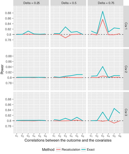
Anyway, apart from these few instances, the proposed sample size recalculation procedure performs very well, with empirical power close to the target level. For example, if only those scenarios with a total exact sample size $\ge 30$$\ge 30$ (i.e., $15$$15$ subjects per group) are considered, the empirical power of the recalculation procedure ranges from $0.79850$$0.79850$ to $0.80272$$0.80272$. Moreover, observe that the simulated power for the recalculation procedure is most of the time closer to the target level of $0.8$$0.8$ than the exact power value, even though all parameters were correctly specified (Figure 1). With respect to the sample sizes, the recalculation procedure yields expected final sample sizes which exceed the exact values by $6$$6$ to $7$$7$ subjects on average (for details, see figures 1 to 3 and Tables 6 to 8 in Section 2 of the Supplementary Material). Similar results have been found for the ANCOVA model with one covariate, as reported by Friede and Kieser (Friede and Kieser 2011). So, even in the case of $c=2$$c=2$ covariates, the overall “price” one has to pay for the increased flexibility of the recalculation procedure is small, thus rendering the proposed method useful for practical applications. However, one has to keep in mind that, especially in small samples, the maximum final sample size resulting from the recalculation procedure could exceed the initially planned sample size considerably. For example, when the total exact sample size in the fixed scenario is 18, the final sample size of the recalculation procedure exceeds the exact sample size by a factor of at least 2 in about 15 percent of simulation runs. However, as the total sample size grows, the proportions drop below $1$$1$ percent in most scenarios. In addition to that, the frequencies of more severe excesses (i.e., by a factor of $3$$3$ or $4$$4$) decrease rapidly, too. Hence, taking $4N_{init}$$4N_{init}$ or $3N_{init}$$3N_{init}$ as an upper bound for the final sample size of the recalculation procedure in fact only represents a slight modification compared to imposing no restriction at all. The simulation results also indicate that the cutoff $2N_{init}$$2N_{init}$ could be used as a safeguard against severe excesses of the exact sample size, which might result from the small-sample variability of the variance estimator. On the other hand, however, this restriction would also carry some risk of power loss. Detailed results are provided in figures 1–3 and Tables 6–8 in Section 2 of the Supplementary Material.

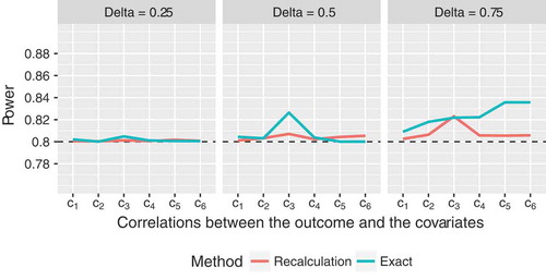
Basically, compared to the balanced settings, the performance for $\gamma =2$$\gamma =2$ is similar, if not even slightly better. The empirical type I error rates are close to the nominal level (median $0.02506$$0.02506$, range $0.02456-0.02558$$0.02456-0.02558$). The maximum deviations from the target power are even smaller than in the balanced settings, and the empirical power always lies above $0.8$$0.8$ now (median empirical power $0.80287$$0.80287$, range $0.80041-0.82300$$0.80041-0.82300$; see Figure 2 for details). Especially for $\mathrm{\Delta }=0.75$$\mathrm{\Delta }=0.75$, the exact power substantially exceeds the target value, whereas the deviation of the power of the recalculation method is much smaller (Figure 2). However, if human and financial resources are limited, the increased probability of exceeding the exact sample size by a factor of 2 or more could pose some difficulties (Table 9 in Section 2 of the Supplementary Material). Apart from that, overall, the comparison between the fixed exact sample sizes and the final recalculated sample sizes yielded similar results as in the balanced setting (figure 4 and Table 9 in Section 2 of the Supplementary Material).

Figure 2. Empirical power of the proposed sample size recalculation procedure vs. exact power in the fixed sample size design with correct specification of nuisance parameters for target power $0.8$$0.8$, assuming a compound symmetry structure of the covariance matrix of the $c=2$$c=2$ covariates, where ${\sigma }_Z=1$${\sigma }_Z=1$ and ${\rho }_Z=0.5$${\rho }_Z=0.5$, and unbalanced group sizes, $n_2=2n_1$$n_2=2n_1$. The labels on the $x$$x$ axis denote the correlations between the outcome and covariate $j$$j$, $j\in \{1,2\}$$j\in \{1,2\}$: $c_1=(0.25,0.25)$$c_1=(0.25,0.25)$, $c_2=(0.5,0.5)$$c_2=(0.5,0.5)$, $c_3=(0.75,0.75)$$c_3=(0.75,0.75)$, $c_4=(0.25,0.5)$$c_4=(0.25,0.5)$, $c_5=(0.25,0.75)$$c_5=(0.25,0.75)$, $c_6=(0.5,0.75)$$c_6=(0.5,0.75)$.

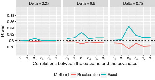
In case of balanced designs with $c=3$$c=3$ covariates, the proposed sample size reassessment procedure yields empirical power values which are consistently slightly smaller than $0.8$$0.8$ (Figure 3). While the method still performs well for $\mathrm{\Delta }\in \{0.25,0.5\}$$\mathrm{\Delta }\in \{0.25,0.5\}$, there is some power loss for $\mathrm{\Delta }=0.75$$\mathrm{\Delta }=0.75$ in most cases (e.g., empirical power of $0.77424$$0.77424$ for ${\sigma }_{YZ}=(0.75,0.75,0.5{)}^{\prime }$${\sigma }_{YZ}=(0.75,0.75,0.5{)}^{\prime }$; Figure 3). However, the type I error rates are still close to the pre-specified level for all scenarios (median $0.02501$$0.02501$, range $0.02472-0.02527$$0.02472-0.02527$). Compared to the scenarios with $c=2$$c=2$ covariates, the discrepancies between exact and recalculated sample sizes appear to be slightly smaller (Figure 5 and Table 10 in Section 2 of the Supplementary Material).

Figure 3. Empirical power of the proposed sample size recalculation procedure vs. exact power in the fixed sample size design with correct specification of nuisance parameters for target power $0.8$$0.8$, assuming an ANCOVA model with $c=3$$c=3$ covariates, a compound symmetry structure of the covariance matrix of the covariates, where ${\sigma }_Z=1$${\sigma }_Z=1$ and ${\rho }_Z=0.5$${\rho }_Z=0.5$, and balanced group sizes, $n_1=n_2$$n_1=n_2$. The labels on the $x$$x$ axis denote the correlations between the outcome and covariate $j$$j$, $j\in \{1,2,3\}$$j\in \{1,2,3\}$: $c_1=(0.25,0.25,0.5)$$c_1=(0.25,0.25,0.5)$, $c_2=(0.5,0.5,0.5)$$c_2=(0.5,0.5,0.5)$, $c_3=(0.75,0.75,0.5)$$c_3=(0.75,0.75,0.5)$, $c_4=(0.25,0.5,0.5)$$c_4=(0.25,0.5,0.5)$, $c_5=(0.25,0.75,0.5)$$c_5=(0.25,0.75,0.5)$, $c_6=(0.5,0.75,0.5)$$c_6=(0.5,0.75,0.5)$.

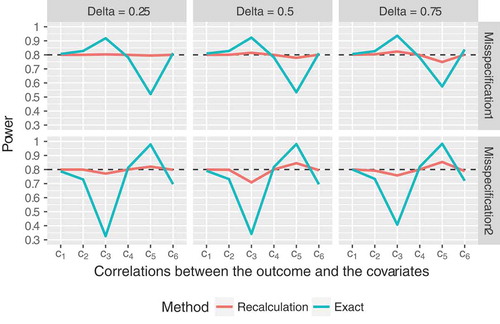
So far, we have only considered somewhat idealistic settings, assuming that the nuisance parameters were correctly specified in advance. In these scenarios, where a fixed sample size calculation approach is supposed to yield reliable results, the recalculation procedure performed equally well and was even slightly superior in some cases. Additionally, we consider two settings now, that more closely mirror the situation commonly faced in practice, namely that the covariance matrix ${\mathrm{\Sigma }}_Z$${\mathrm{\Sigma }}_Z$ of the covariates is misspecified. Here the advantages of the increased flexibility due to the interim reassessment become even more obvious. On the one hand, we assumed that initially, ${\rho }_Z$${\rho }_Z$ was set to $0.75$$0.75$, but the true value was $0.5$$0.5$. On the other hand, instead of ${\rho }_Z=0.75$${\rho }_Z=0.75$, we used ${\rho }_Z=0.25$${\rho }_Z=0.25$ for the initial sample size calculation. It can be seen in Figure 4 that our proposed recalculation procedure outperformed the fixed sample size calculation method in most scenarios. The latter led to either substantially over- or underpowered results, depending on the configuration of the covariances between the covariates and the outcome. The sample size reassessment procedure was slightly underpowered for covariance scenario $c_3$$c_3$ (i.e., strong correlations between the outcomes and the covariates, which in turn translates to small sample sizes) and misspecification scenario 2 (i.e., assuming that ${\rho }_Z$${\rho }_Z$ was equal to $0.25$$0.25$ instead of $0.75$$0.75$). However, it clearly outperformed the fixed sample size calculation method, which totally failed in that scenario. Moreover, similar to all previously discussed settings, our proposed method again keeps the $\alpha$$\alpha$ level well (median $0.02498$$0.02498$, range $0.02466-0.02568$$0.02466-0.02568$).

Figure 4. Empirical power of the proposed sample size recalculation procedure vs. exact power in the fixed sample size design for target power $0.8$$0.8$ in case of $c=2$$c=2$ covariates, assuming ${\sigma }_Z=1$${\sigma }_Z=1$, and balanced group sizes, $n_1=n_2$$n_1=n_2$. The labels on the $x$$x$ axis denote the correlations between the outcome and covariate $j$$j$, $j\in \{1,2\}$$j\in \{1,2\}$: $c_1=(0.25,0.25)$$c_1=(0.25,0.25)$, $c_2=(0.5,0.5)$$c_2=(0.5,0.5)$, $c_3=(0.75,0.75)$$c_3=(0.75,0.75)$, $c_4=(0.25,0.5)$$c_4=(0.25,0.5)$, $c_5=(0.25,0.75)$$c_5=(0.25,0.75)$, $c_6=(0.5,0.75)$$c_6=(0.5,0.75)$. Misspecification 1: ${\rho }_Z=0.75$${\rho }_Z=0.75$ was assumed for sample size calculation for the fixed design and initial sample size calculation of the recalculation procedure, although the true correlation was $0.5$$0.5$. Misspecification 2: ${\rho }_Z=0.25$${\rho }_Z=0.25$ was assumed, although the true correlation was $0.75$$0.75$.

4. Application to a real-life setting

In order to illustrate the application of our proposed sample size recalculation procedure, we use data from the SIESTA (Sedation vs. Intubation for Endovascular Stroke TreAtment) trial. In this monocentric randomized parallel-group trial, the main aim was to assess if conscious sedation is superior to general anesthesia for early neurological improvement among patients receiving stroke thrombectomy. The change from baseline of the National Institutes of Health Stroke Scale (NIHSS) 24 hours after the intervention was considered as the primary outcome, which was compared between the two groups while adjusting for the NIHSS at baseline. For further details, we refer to the original publication of the results (Schönenberger et al. 2016). Regarding sample size calculation, the investigators report that the estimated variances, which were obtained from previous studies, showed considerable variation. Even worse, an estimate of the correlation between the outcome and the NIHSS at baseline was not available at all. Therefore, it was decided to conduct a preliminary sample size calculation with the $t$$t$-test formula, which yielded a total sample size $N=100$$N=100$, assuming equal group allocation. When data of $75$$75$ patients were available (i.e., $\tau =0.75$$\tau =0.75$), a pre-planned blinded sample size recalculation was carried out, using the method proposed by Friede and Kieser (Friede and Kieser 2011). Further details are provided in the study protocol (Schönenberger et al. 2015).

Clearly, this is a case where an interim sample size reassessment is more appropriate than calculating sample sizes at the planning stage and keeping them fixed throughout the conduct of the study. The latter approach would have to rely on a somewhat arbitrary initial guess of the correlation and on a variance estimate which is subject to considerable uncertainty. So, the method employed in the SIESTA study was definitely a good choice. Nevertheless, we shall examine whether the final sample size would have substantially changed if multiple covariates had been considered. Note that such a recalculation procedure could not be implemented in the SIESTA trial as the methodology was not available at that time, but is presented in this article. At this point, we would like to mention that the primary outcome as well as some of the covariates, which will be considered below, are ordinally scaled variables. However, for the classical ANCOVA as well as for our proposed method to be applied, normally distributed variables are required. Since there is some evidence that type I error rates and power are not substantially affected by applying the classical ANCOVA to ordinally scaled outcomes and baseline measurements thereof (Sullivan and D’Agostino 2003), it is appropriate to use the data for illustrating the application of our proposed sample size recalculation method. Nevertheless, we would like to emphasize that the resulting effect sizes (i.e., adjusted mean differences) should be interpreted with caution if the outcome and/or the covariates are ordinally scaled.

In the sequel, we perform several sample size recalculations based on the original data available at the time of the interim analysis, assuming a group allocation ratio $\gamma =1$$\gamma =1$ and a clinically relevant difference $\mathrm{\Delta }=4$$\mathrm{\Delta }=4$. We set $\alpha =0.05$$\alpha =0.05$ and $1-\beta =0.9$$1-\beta =0.9$. These specifications correspond to the setup described in the study protocol; however, unlike there, we do not impose an upper bound on the final sample size because this would complicate the assessment of potential differences between the respective models. For sample size recalculation, we conducted steps 2 and 3 from Section 2.2. At first, we reproduced the sample size reassessment that had been actually carried out in the study, assuming an ANCOVA model with one single covariate, namely NIHSS at baseline. The estimated residual variance and final sample size were ${\hat{\sigma }}_{\tau }^2=99.35$${\hat{\sigma }}_{\tau }^2=99.35$ and ${\hat{N}}_{rec}=264$${\hat{N}}_{rec}=264$, respectively. Next, we added the age of the patients (in years) as a second covariate. Using this model, both values slightly decreased (${\hat{\sigma }}_{\tau }^2=96.99$${\hat{\sigma }}_{\tau }^2=96.99$, ${\hat{N}}_{rec}=258$${\hat{N}}_{rec}=258$). As an alternative, we considered replacing age by the degree of recanalization, as quantified by the Thrombolysis In Cerebral Infarction (TICI) scale. So, again, we had a scenario with $c=2$$c=2$ covariates, namely NIHSS at baseline and TICI. Obviously, the inclusion of TICI led to a substantial decrease in the final sample size down to ${\hat{N}}_{rec}=214$${\hat{N}}_{rec}=214$ (${\hat{\sigma }}_{\tau }^2=80.42$${\hat{\sigma }}_{\tau }^2=80.42$). Finally, we added the door-to-intervention time (in seconds) to the model. Taking NIHSS at baseline, TICI and door-to-intervention time as covariates, we got ${\hat{\sigma }}_{\tau }^2=77.43$${\hat{\sigma }}_{\tau }^2=77.43$ and ${\hat{N}}_{rec}=206$${\hat{N}}_{rec}=206$, respectively.

Summing up, we would like to emphasize three important points. Firstly, we have seen that in all scenarios the recalculated sample sizes substantially exceeded the initially planned sample size $N=100$$N=100$. Secondly, the differences in final sample sizes for various choices of the covariates might indicate that careful thoughts about the associations between the outcome and potential covariates are required in the planning phase. In the example, the inclusion of TICI led to a considerable decrease in the final sample size, whereas there was hardly any use in adding age to the model. Thirdly, it seems as if increasing the number of covariates beyond $c=2$$c=2$ would not lead to further substantial improvements, which is consistent with findings in a similar repeated measures context (Frison and Pocock 1992). However, we would like to emphasize that our example is supposed to serve of course merely as an illustration of how to apply our proposed method. Needless to say that compared to evidence from simulations, the generalizability of the findings is thus limited.

5. Discussion and conclusions

Although some work concerning exact and approximate sample size calculation in the context of an ANCOVA model with multiple covariates has been published recently, there is currently no method available, which allows for blinded sample size recalculation in that setting. We have proposed such a method here, which is based on the approach suggested by Friede and Kieser (Friede and Kieser 2011) for the situation of one single covariate. At the time point of the blinded interim reassessment, the residual variance is estimated based on the pooled interim data, and the final sample size is recalculated accordingly. The results of our extensive simulation study indicate that even if all parameters are correctly specified, the performance of the blinded recalculation method is close to the exact results for models with 2 random covariates and for most scenarios with 3 covariates, except in cases where the required sample size is very small (i.e., for standardized effects $\mathrm{\Delta }=0.75$$\mathrm{\Delta }=0.75$). In more realistic scenarios, where initial misspecifications of a nuisance parameter are present, our proposed method is clearly superior to the fixed approach. Apart from that, regardless whether a fixed sample size calculation formula or a recalculation method is employed, caution is needed when initially specifying the values of the nuisance parameters in order to prevent the sample sizes provided by the formula from being negative. This note of caution is important and has to be taken into consideration when applying the aforementioned methods in real-life settings (e.g., by checking for positive semidefiniteness of the joint covariance matrix).

The sample size calculation formulas, which are used in our proposed procedure, have been derived assuming a multivariate normal distribution of the covariates and the outcome. However, in applied research, this assumption is frequently violated. The outcome and/or the covariates may not even be continuous (e.g., ordinal scores like the modified Rankin Scale (Van de Graaf et al. 2018), the Hamilton Rating Scale for Depression (Kasper et al. 2006), etc.). We have already touched this issue briefly in Section 4 providing some explanation on how the ANCOVA results can be used and interpreted, though. In such instances, however, using nonparametric ANCOVA methods (Bathke and Brunner 2003) would be an attractive alternative with respect to the interpretation and the robustness of the results. Nevertheless, for parallel-group comparisons, sample size calculation methods are only available for the unadjusted Wilcoxon-Mann-Whitney test (Govindarajulu 2007; Noether 1987). Therefore, investigating sample size (re-)calculation procedures for nonparametric ANCOVA is a promising goal of future research.

Basically, our proposed recalculation method can be applied to ANCOVA models with an abitrary number of covariates. However, we restricted to a thorough examination of various settings with $c=2$$c=2$ and $c=3$$c=3$ as well as balanced and unbalanced scenarios. Evidence from repeated measures models indicates that if the number of baseline visits is increased, there is always a reduction of the required sample size (i.e., a gain in power). However, the magnitude of that reduction decreases considerably with a growing number of baseline visits (Frison and Pocock 1992). In our simulation study, we also noticed that already for $c=3$$c=3$ the reduction in sample sizes compared to a similar scenario for $c=2$$c=2$ was not larger than 10 in most cases. Moreover, especially in small to moderate samples, multicollinearity issues are more likely to occur with an increasing number of covariates. Therefore, all in all, we recommend including at most $3$$3$ covariates into the model, thus maintaining a balance between gains in power and feasibility in practical applications.

It should generally be noted that any blinded reassessment procedure cannot correct for misspecified effect sizes. For this purpose, an adaptive design with unblinded interim analysis would be an appealing alternative. However, such a method has the disadvantage that unblinding and, thus, establishing an independent data analysis group, whose members must not be involved in the trial otherwise, is required. Furthermore, regulatory guidelines prefer blinded sample size reassessment due to avoiding bias (European Medicines Agency 2007; Food and Drug Administration 2016, 2018). Apart from that, we have to acknowledge that type I error control was only examined empirically in the present work. While from a formal point of view this might be somewhat suboptimal, it should be mentioned that analytical solutions can only be obtained in rather simple settings (e.g., for the two-sample $t$$t$-test, see Kieser and Friede (2003)). Moreover, in a recent draft guidance of the FDA, it is stated that assessing type I error control by means of simulations might be appropriate (Food and Drug Administration 2018). Anyway, due to the fact that it is of course not possible to cover all potentially relevant scenarios in the present manuscript, we recommend performing some simulations for the particular setting one is interested in before actually using the results of our proposed recalculation procedure for study planning purposes.

To conclude, firstly, we have assessed the performance of several approximate fixed sample size calculation approaches in terms of sample size and power. According to the results of the simulation studies, the proposed adjustments, which take the number of covariates into account, are easy to apply and can be safely used in practice. Moreover, most importantly, we have proposed a blinded sample size recalculation method for an ANCOVA model with multiple random covariates and showed by extensive simulations that it maintains the pre-specified type I error level and achieves the desired power very well in models with $2$$2$ or $3$$3$ covariates, except for very small sample sizes. In case of initial misspecifications, our proposed method clearly outperforms the fixed sample size calculation approach. Thus, applied researchers now have a procedure at hand, which is easy to use and increases the robustness of sample size calculation while at the same time keeping the treatment allocation blinded.

Conflict of interest

The authors declare no potential conflict of interests.

Supporting information

The following supporting information is available as part of the online article:

SSRE_multiple_Ancova.R This file contains the implementation of several fixed sample size calculation approaches and the proposed re-calculation procedure as well as a function to check the initially specified covariance structure in R.

SSRE_multiple_Ancova_Supplement.pdf This document contains additional simulation results for the fixed sample size calculation settings discussed in the manuscript as well as for our proposed recalculation procedure. Regarding the latter, a particular focus is set on the distribution of the sample sizes.

Acknowledgments

We would like to thank the investigators of the SIESTA trial for providing the data for the example discussed in our manuscript. The present work was supported by the Austrian Science Fund (FWF), grant I 2697-N31.

Supplementary material

Supplementary material can be accessed here.

Additional information

Funding

This work was supported by the Austrian Science Fund [I 2697-N31].

Appendix

Derivation of the basic approximate sample size formula (3) in Section 2

At first, we rewrite the test statistic $T$$T$ defined in (1) as

$T=\frac{\hat{\mathrm{\Delta }}}{\sqrt{\left(n_1^{-1}+n_2^{-1}+{\hat{Q}}_Z\right)\kappa {\hat{Q}}_{YZ}}},$$T=\frac{\hat{\mathrm{\Delta }}}{\sqrt{\left(n_1^{-1}+n_2^{-1}+{\hat{Q}}_Z\right)\kappa {\hat{Q}}_{YZ}}},$

where ${\hat{Q}}_Z:={\bar{\mathbf{Z}}}_d^{\prime }{\left((n_1+n_2-2){\hat{\mathrm{\Sigma }}}_Z\right)}^{-1}{\bar{\mathbf{Z}}}_d$${\hat{Q}}_Z:={\bar{\mathbf{Z}}}_d^{\prime }{\left((n_1+n_2-2){\hat{\mathrm{\Sigma }}}_Z\right)}^{-1}{\bar{\mathbf{Z}}}_d$, $\hat{\mathrm{\Delta }}:={\hat{\mu }}_1-{\hat{\mu }}_2$$\hat{\mathrm{\Delta }}:={\hat{\mu }}_1-{\hat{\mu }}_2$, $\kappa :=(n_1+n_2-2)/(n_1+n_2-2-c)$$\kappa :=(n_1+n_2-2)/(n_1+n_2-2-c)$, ${\hat{Q}}_{YZ}:={\hat{\sigma }}_Y^2$${\hat{Q}}_{YZ}:={\hat{\sigma }}_Y^2$ $(1-{\hat{\sigma }}_Y^{-2}{\hat{\mathit{\sigma }}}_{YZ}^{\prime }{\hat{\mathrm{\Sigma }}}_Z^{-1}{\hat{\mathit{\sigma }}}_{YZ})$$(1-{\hat{\sigma }}_Y^{-2}{\hat{\mathit{\sigma }}}_{YZ}^{\prime }{\hat{\mathrm{\Sigma }}}_Z^{-1}{\hat{\mathit{\sigma }}}_{YZ})$.

Recall that under $H_0$$H_0$, $T$$T$ has a central $t$$t$-distribution with $n_1+n_2-2-c$$n_1+n_2-2-c$ degrees of freedom. In order to obtain the distribution of $T$$T$ under the fixed alternative $H_1:{\mu }_1-{\mu }_2=\mathrm{\Delta }>0$$H_1:{\mu }_1-{\mu }_2=\mathrm{\Delta }>0$, let $Q_{YZ}:={\sigma }_Y^2(1-{\mathit{\sigma }}_{YZ}^{\prime }{\mathrm{\Sigma }}_Z^{-1}{\mathit{\sigma }}_{YZ}/{\sigma }_Y^2)$$Q_{YZ}:={\sigma }_Y^2(1-{\mathit{\sigma }}_{YZ}^{\prime }{\mathrm{\Sigma }}_Z^{-1}{\mathit{\sigma }}_{YZ}/{\sigma }_Y^2)$, and ${\sigma }_Y^2$${\sigma }_Y^2$, ${\sigma }_{YZ}$${\sigma }_{YZ}$, and ${\mathrm{\Sigma }}_Z$${\mathrm{\Sigma }}_Z$ denote the variance of the outcome, the $c$$c$-dimensional vector containing the covariances between the outcome and the covariates, and the covariance matrix of the covariates, respectively. We rewrite the test statistic $T$$T$ as follows:

$\begin{array}{rl}& T=\frac{\hat{\mathrm{\Delta }}}{\sqrt{\left(n_1^{-1}+n_2^{-1}+{\hat{Q}}_Z\right)\kappa {\hat{Q}}_{YZ}}}\\ & =\frac{\left(\left(\hat{\mathrm{\Delta }}-\mathrm{\Delta }\right)+\mathrm{\Delta }\right)/\sqrt{n_1^{-1}+n_2^{-1}+{\hat{Q}}_Z}}{\sqrt{\kappa {\hat{Q}}_{YZ}}}\\ & =\frac{\left(\hat{\mathrm{\Delta }}-\mathrm{\Delta }\right)/\sqrt{\left(n_1^{-1}+n_2^{-1}+{\hat{Q}}_Z\right)Q_{YZ}}+\mathrm{\Delta }/\sqrt{\left(n_1^{-1}+n_2^{-1}+{\hat{Q}}_Z\right)Q_{YZ}}}{\sqrt{\kappa {\hat{Q}}_{YZ}/Q_{YZ}}}.\end{array}$$\begin{array}{rl}& T=\frac{\hat{\mathrm{\Delta }}}{\sqrt{\left(n_1^{-1}+n_2^{-1}+{\hat{Q}}_Z\right)\kappa {\hat{Q}}_{YZ}}}\\ & =\frac{\left(\left(\hat{\mathrm{\Delta }}-\mathrm{\Delta }\right)+\mathrm{\Delta }\right)/\sqrt{n_1^{-1}+n_2^{-1}+{\hat{Q}}_Z}}{\sqrt{\kappa {\hat{Q}}_{YZ}}}\\ & =\frac{\left(\hat{\mathrm{\Delta }}-\mathrm{\Delta }\right)/\sqrt{\left(n_1^{-1}+n_2^{-1}+{\hat{Q}}_Z\right)Q_{YZ}}+\mathrm{\Delta }/\sqrt{\left(n_1^{-1}+n_2^{-1}+{\hat{Q}}_Z\right)Q_{YZ}}}{\sqrt{\kappa {\hat{Q}}_{YZ}/Q_{YZ}}}.\end{array}$

Observe that $Q_{YZ}$$Q_{YZ}$ is just the residual variance of the ANCOVA model (Ravishanker and Dey 2002, p.156), and $\kappa {\hat{Q}}_{YZ}$$\kappa {\hat{Q}}_{YZ}$ is the corresponding residual variance estimator. Moreover, straightforward calculations show that $Var(\hat{\mathrm{\Delta }})=Var({\hat{\mu }}_1-{\hat{\mu }}_2)=\sqrt{\left(n_1^{-1}+n_2^{-1}+{\hat{Q}}_Z\right)Q_{YZ}}$$Var(\hat{\mathrm{\Delta }})=Var({\hat{\mu }}_1-{\hat{\mu }}_2)=\sqrt{\left(n_1^{-1}+n_2^{-1}+{\hat{Q}}_Z\right)Q_{YZ}}$. Hence, under $H_1:{\mu }_1-{\mu }_2=\mathrm{\Delta }>0$$H_1:{\mu }_1-{\mu }_2=\mathrm{\Delta }>0$, the test statistic $T$$T$ has a non-central $t$$t$-distribution with $n_1+n_2-2-c$$n_1+n_2-2-c$ degrees of freedom and non-centrality parameter

(7) $\delta =\frac{\mathrm{\Delta }}{\sqrt{\left({\hat{Q}}_Z+n_1^{-1}+n_2^{-1}\right)Q_{YZ}}}.$$\delta =\frac{\mathrm{\Delta }}{\sqrt{\left({\hat{Q}}_Z+n_1^{-1}+n_2^{-1}\right)Q_{YZ}}}.$(7)

Now, in order to achieve the target power $1-\beta$$1-\beta$ at the nominal type I error level $\alpha /2$$\alpha /2$, the equation

$t_{1-\alpha /2,n_1+n_2-2-c,0}=t_{\beta ,n_1+n_2-2-c,\delta }$$t_{1-\alpha /2,n_1+n_2-2-c,0}=t_{\beta ,n_1+n_2-2-c,\delta }$

has to hold, where $t_{p,df,nc}$$t_{p,df,nc}$ denotes the $p$$p$–quantile of the $t$$t$-distribution with $df$$df$ degrees of freedom and non-centrality parameter $nc$$nc$. Hence, since $t_{\beta ,n_1+n_2-2-c,\delta }\approx t_{\beta ,n_1+n_2-2-c,0}+\delta$$t_{\beta ,n_1+n_2-2-c,\delta }\approx t_{\beta ,n_1+n_2-2-c,0}+\delta$, we get

$t_{1-\alpha /2,n_1+n_2-2-c,0}\approx t_{\beta ,n_1+n_2-2-c,0}+\delta$$t_{1-\alpha /2,n_1+n_2-2-c,0}\approx t_{\beta ,n_1+n_2-2-c,0}+\delta$

For “large” sample sizes, we can approximate the $t$$t$-quantiles by their standard normal counterparts. Hence, some straightforward algebra yields

(8) ${\delta }^2\approx {\left(z_{1-\alpha /2}+z_{1-\beta }\right)}^2.$${\delta }^2\approx {\left(z_{1-\alpha /2}+z_{1-\beta }\right)}^2.$(8)

By using $n_2=\gamma n_1$$n_2=\gamma n_1$ and plugging in the expression from (7) for $\delta$$\delta$, we obtain

$\begin{array}{rl}& \frac{{\mathrm{\Delta }}^2}{\left(n_1^{-1}+n_2^{-1}+{\hat{Q}}_Z\right)Q_{YZ}}\approx {\left(z_{1-\alpha /2}+z_{1-\beta }\right)}^2\\ & \iff \frac{{\mathrm{\Delta }}^2}{{\left(\gamma n_1\right)}^{-1}\left(\gamma +1+\gamma n_1{\hat{Q}}_Z\right)}\approx {\left(z_{1-\alpha /2}+z_{1-\beta }\right)}^2{Q}_{YZ}\\ & \iff \gamma n_1{\mathrm{\Delta }}^2\approx {\left(z_{1-\alpha /2}+z_{1-\beta }\right)}^2{Q}_{YZ}\left(\gamma +1+\gamma n_1{\hat{Q}}_Z\right)\\ & \iff n_1\left(1-{\left(z_{1-\alpha /2}+z_{1-\beta }\right)}^2{Q}_{YZ}{\hat{Q}}_Z/{\mathrm{\Delta }}^2\right)\approx {\left(z_{1-\alpha /2}+z_{1-\beta }\right)}^2{Q}_{YZ}\left(\gamma +1\right)/\left(\gamma {\mathrm{\Delta }}^2\right).(9)\end{array}$$\begin{array}{rl}& \frac{{\mathrm{\Delta }}^2}{\left(n_1^{-1}+n_2^{-1}+{\hat{Q}}_Z\right)Q_{YZ}}\approx {\left(z_{1-\alpha /2}+z_{1-\beta }\right)}^2\\ & \iff \frac{{\mathrm{\Delta }}^2}{{\left(\gamma n_1\right)}^{-1}\left(\gamma +1+\gamma n_1{\hat{Q}}_Z\right)}\approx {\left(z_{1-\alpha /2}+z_{1-\beta }\right)}^2{Q}_{YZ}\\ & \iff \gamma n_1{\mathrm{\Delta }}^2\approx {\left(z_{1-\alpha /2}+z_{1-\beta }\right)}^2{Q}_{YZ}\left(\gamma +1+\gamma n_1{\hat{Q}}_Z\right)\\ & \iff n_1\left(1-{\left(z_{1-\alpha /2}+z_{1-\beta }\right)}^2{Q}_{YZ}{\hat{Q}}_Z/{\mathrm{\Delta }}^2\right)\approx {\left(z_{1-\alpha /2}+z_{1-\beta }\right)}^2{Q}_{YZ}\left(\gamma +1\right)/\left(\gamma {\mathrm{\Delta }}^2\right).(9)\end{array}$

Now, observe that ${\hat{Q}}_Z$${\hat{Q}}_Z$ is most likely close to 0: ${\bar{\mathbf{Z}}}_d$${\bar{\mathbf{Z}}}_d$ is supposed to be small for reasonable sample sizes, since the covariate means of the populations are equal to ${\mu }_Z$${\mu }_Z$ for both groups. Moreover, the elements of the inverse of ${\hat{\mathrm{\Sigma }}}_Z$${\hat{\mathrm{\Sigma }}}_Z$ will be small, too, unless the variances are close to 0, or the covariates exhibit strong linear dependencies. As either scenario would lead to potentially serious problems regarding inference, these cases can be excluded. Moreover, observe that the factor ${\left(n_1+n_2-2\right)}^{-1}$${\left(n_1+n_2-2\right)}^{-1}$ leads to a further deflation of the quantity ${\hat{Q}}_Z$${\hat{Q}}_Z$. Hence, it might be appropriate to drop the term ${\left(z_{1-\alpha /2}+z_{1-\beta }\right)}^2{Q}_{YZ}{\hat{Q}}_Z/{\mathrm{\Delta }}^2$${\left(z_{1-\alpha /2}+z_{1-\beta }\right)}^2{Q}_{YZ}{\hat{Q}}_Z/{\mathrm{\Delta }}^2$. Thus, we can further simplify (9) to

$n_1\approx \frac{{\left(z_{1-\alpha /2}+z_{1-\beta }\right)}^2{Q}_{YZ}\left(\gamma +1\right)}{\gamma {\mathrm{\Delta }}^2}.$$n_1\approx \frac{{\left(z_{1-\alpha /2}+z_{1-\beta }\right)}^2{Q}_{YZ}\left(\gamma +1\right)}{\gamma {\mathrm{\Delta }}^2}.$

Finally, observe that $Q_{YZ}={\sigma }_Y^2(1-{\sigma }_Y^{-2}{\sigma }_{YZ}^{\prime }{\mathrm{\Sigma }}_Z^{-1}{\sigma }_{YZ})={\sigma }_Y^2(1-R^2)$$Q_{YZ}={\sigma }_Y^2(1-{\sigma }_Y^{-2}{\sigma }_{YZ}^{\prime }{\mathrm{\Sigma }}_Z^{-1}{\sigma }_{YZ})={\sigma }_Y^2(1-R^2)$, according to the definition of $Q_{YZ}$$Q_{YZ}$. Hence,

$N=n_1+n_2=n_1\left(\gamma +1\right)\approx \frac{{\left(z_{1-\alpha /2}+z_{1-\beta }\right)}^2{\sigma }_Y^2\left(1-R^2\right)\left(\gamma +1\right)}{\gamma {\mathrm{\Delta }}^2}\left(\gamma +1\right).$$N=n_1+n_2=n_1\left(\gamma +1\right)\approx \frac{{\left(z_{1-\alpha /2}+z_{1-\beta }\right)}^2{\sigma }_Y^2\left(1-R^2\right)\left(\gamma +1\right)}{\gamma {\mathrm{\Delta }}^2}\left(\gamma +1\right).$

This completes the derivation of (3).

Some remarks regarding formulas (5) and (6)

The approximate formulas (5) and (6) can be motivated by some heuristic arguments: Structurally, the non-centrality parameter $\delta$$\delta$ in equation (7) looks very similar to the test statistic $T$$T$. In fact, the latter can be obtained from the former by plugging in the respective estimators for the population quantities. However, observe that $Q_{YZ}$$Q_{YZ}$ is replaced by $\kappa {\hat{Q}}_{YZ}$$\kappa {\hat{Q}}_{YZ}$ then, where $\kappa =(N-2)/(N-2-c)$$\kappa =(N-2)/(N-2-c)$ with $N=n_1+n_2$$N=n_1+n_2$. Therefore, it may be sensible to apply a corresponding post-hoc “finite sample”-adjustment of the approximate sample size $N_A$$N_A$. It should be noted, however, that the DF adjustment is “stronger” than the GS adjustment for $c\ge 2$$c\ge 2$ and typical choices of $\alpha$$\alpha$, because

$N_{DF}=N_A+c+\frac{c^2+2c}{N_A-2-c}.$$N_{DF}=N_A+c+\frac{c^2+2c}{N_A-2-c}.$

For example, for $\alpha =0.05$$\alpha =0.05$ we have

$z_{1-\alpha /2}^2/2\approx 1.921<2\le c$$z_{1-\alpha /2}^2/2\approx 1.921<2\le c$

for $c\ge 2$$c\ge 2$. It can also be seen from the previous calculations that the difference might actually be small in most practically relevant settings, especially as upward rounding has to be taken into account, too. Therefore, it could be sensible to apply an even stronger adjustment of $N_A$$N_A$ by combining GS and DF, as proposed in (6). Anyway, a common feature of (5) and (6) is that, in contrast to the GS adjustment, the number of covariates is taken into account. It has been argued that one of the major drawbacks of using (3) or (4) was that the number of covariates did not play a role (Shieh 2017). Therefore, it seems plausible that the performance can be improved by applying adjustments, which take the number of covariates $c$$c$ into account.

References

- Bathke, A., and E. Brunner. 2003. A nonparametric alternative to analysis of covariance. In Recent advances and trends in nonparametric statistics, ed. M. Akritas and D. Politis, 109–120. Amsterdam: JAI.
- Bauer, P., F. Bretz, V. Dragalin, F. König, and G. Wassmer. 2015. Twenty-five years of confirmatory adaptive designs: Opportunities and pitfalls. Stat Med 35:325–347. doi:10.1002/sim.6472.
- Borm, G., J. Fransen, and W. Lemmens. 2007. A simple sample size formula for analysis of covariance in randomized clinical trials. J Clin Epidemiol 60 (12):1234–1238. doi:10.1016/j.jclinepi.2007.02.006.
- Chi, Y., D. Glueck, and K. Muller. 2018. Power and sample size for fixed-effects inference in reversible linear mixed models. Am Stat. accepted. doi: 10.1080/00031305.2017.1415972.
- Dasgupta, A., S. Zhang, L. Thabane, and P. Nair. 2013. Sample sizes for clinical trials using sputum eosinophils as a primary outcome. Eur Respir J 42 (4):1003–1011. doi:10.1183/09031936.00075712.
- European Medicines Agency. 2007. Reflection paper on methodological issues in confirmatory clinical trials planned with an adaptive design CHMP/EWP/2459/02. https://www.ema.europa.eu/en/documents/scientific-guideline/reflection-paper-methodological-issues-confirmatory-clinical-trials-planned-adaptive-design_en.pdf
- European Medicines Agency. 2015. Guideline on adjustment for baseline covariates in clinical trials EMA/CHMP/295050/2013. https://www.ema.europa.eu/en/documents/scientific-guideline/draft-guideline-adjustment-baseline-covariates_en.pdf
- Food and Drug Administration. 2016. Adaptive designs for medical device clinical studies (draft guidance). Version of July 2016. https://mdepinet.org/wp-content/uploads/ucm446729.pdf
- Food and Drug Administration. 2018. Adaptive design clinical trials for drugs and biologics (draft guidance). Version of September 2018. https://www.fda.gov/media/78495/download
- Friede, T., and M. Kieser. 2006. Sample size recalculation in internal pilot study designs: A review. Biom J 48 (4):537–555. doi:10.1002/(ISSN)1521-4036.
- Friede, T., and M. Kieser. 2011. Blinded sample size recalculation for clinical trials with normal data and baseline adjusted analysis. Pharm Stat 10:8–13. doi:10.1002/pst.398.
- Friede, T., and M. Kieser. 2013. Blinded sample size re-estimation in superiority and noninferiority trials: Bias versus variance in variance estimation. Pharm Stat 12 (3):141–146. doi:10.1002/pst.1564.
- Frison, L., and S. Pocock. 1992. Repeated measures in clinical trials: Analysis using mean summary statistics and its implications for design. Stat Med 11 (13):1685–1704. doi:10.1002/sim.4780111304.
- Gholizadeh, S., P. Dehgan, S. Mohammad-Alizadeh, A. Aliasgarzadeh, and M. Mirghafourvand. 2018. The effect of resistant dextrin as a prebiotic on metabolic parameters and androgen level in women with polycystic ovarian syndrome: A randomized, triple-blind, controlled, clinical trial. Eur J Nutr 58 (2):629–640.
- Govindarajulu, Z. 2007. Sample size re-estimation: Nonparametric approach. J Stat Theory Pract 1 (2):253–264. doi:10.1080/15598608.2007.10411837.
- Guenther, W. 1981. Sample size formulas for normal theory t tests. Am Stat 35 (4):243–244.
- Haider, S., I. Grabovac, E. Winzer, A. Kapan, K. Schindler, C. Lackinger, S. Titze, and T. Dorner. 2017. Change in inflammatory parameters in prefrail and frail persons obtaining physical training and nutritional support provided by lay volunteers: A randomized controlled trial. PLoS One 12 (10):e0185879. doi:10.1371/journal.pone.0185879.
- Howard, J., K. Utsugisawa, M. Benatar, H. Murai, R. Barohn, I. Illa, S. Jacob, J. Vissing, T. Burns, J. Kissel, et al. 2017. Safety and efficacy of eculizumab in anti-acetylcholine receptor antibody-positive refractory generalised myasthenia gravis (REGAIN): A phase 3, randomised, double-blind, placebo-controlled, multicentre study. Lancet Neurol 16 (12):976–986. doi:10.1016/S1474-4422(17)30122-9.
- Huitema, B. 2011. The Analysis of Covariance and Alternatives: Statistical methods for experiments, quasi-experiments, and single-case studies, New York: Wiley. ISBN 9781118067468.
- International Council for Harmonisation of Technical Requirements for Pharmaceuticals for Human Use. 1998. ICH harmonized tripartite guideline: Statistical principles for clinical trials E9, step 4. https://www.ich.org/fileadmin/Public_Web_Site/ICH_Products/Guidelines/Efficacy/E9/Step4/E9_Guideline.pdf
- Kasper, S., I. Anghelescu, A. Szegedi, A. Dienel, and M. Kieser. 2006. Superior efficacy of St John’s wort extract WS 5570 compared to placebo in patients with major depression: A randomized, double-blind, placebo-controlled, multi-center trial. BMC Med 23 (4):14. doi:10.1186/1741-7015-4-14.
- Kieser, M., and T. Friede. 2003. Simple procedures for blinded sample size adjustment that do not affect the type I error rate. Stat Med 22:3571–3581. doi:10.1002/sim.1585.
- Moher, D., S. Hopewell, K. Schulz, V. Montori, P. Gøtzsche, P. Devereaux, D. Elbourne, M. Egger, and D. Altman. 2010. CONSORT 2010 explanation and elaboration: Updated guidelines for reporting parallel group randomised trials. BMJ 340:c869. doi:10.1136/bmj.c293.
- Noether, G. 1987. Sample size determination for some common nonparametric tests. J Am Stat Assoc 85:645–647. doi:10.1080/01621459.1987.10478478.
- Proschan, M. 2005. Two-stage sample size re-estimation based on a nuisance parameter: A review. J Biopharm Stat 15 (4):559–574. doi:10.1081/BIP-200062852.
- Ravishanker, N., and D. Dey. 2002. A first course in linear model theory. New York: Chapman & Hall/CRC.
- Schönenberger, S., M. Möhlenbruch, J. Pfaff, S. Mundiyanapurath, M. Kieser, M. Bendszus, W. Hacke, and J. Bösel. 2015. Sedation vs. intubation for endovascular stroke treatment (SIESTA) – a randomized monocentric trial. Int J Stroke 10 (6):969–978. doi:10.1111/ijs.12488.
- Schönenberger, S., L. Uhlmann, W. Hacke, S. Schieber, S. Mundiyanapurath, J. Purrucker, S. Nagel, C. Klose, J. Pfaff, M. Bendszus, et al. 2016. Effect of conscious sedation vs general anesthesia on early neurological improvement among patients with ischemic stroke undergoing endovascular thrombectomy: A randomized clinical trial. JAMA 316 (19):1986–1996. doi:10.1001/jama.2016.16623.
- Schouten, H. 1999. Sample size formula with a continuous outcome for unequal group sizes and unequal variances. Stat Med 18 (1):87–91. doi:10.1002/(SICI)1097-0258(19990115)18:1<87::AID-SIM958>3.0.CO;2-K.
- Shieh, G. 2017. Power and sample size calculations for contrast analysis in ANCOVA. Multivariate Behav Res 52 (1):1–11. doi:10.1080/00273171.2016.1219841.
- Sperling, M., P. Klein, and J. Tsai. 2017. Randomized, double-blind, placebo-controlled phase 2 study of ganaxolone as add-on therapy in adults with uncontrolled partial-onset seizures. Epilepsia 58 (4):558–564. doi:10.1111/epi.13705.
- Sugiyama, H., O. Uemura, T. Mori, N. Okisio, K. Unai, and M. Liu. 2017. Effect of imidafenacin on the urodynamic parameters of patients with indwelling bladder catheters due to spinal cord injury. Spinal Cord 55:187–191. doi:10.1038/sc.2016.168.
- Sullivan, L., and R. D’Agostino. 2003. Robustness and power of analysis of covariance applied to ordinal scaled data as arising in randomized controlled trials. Stat Med 22:1317–1334. doi:10.1002/sim.1433.
- Tang, Y. 2018. Exact and approximate power and sample size calculations for analysis of covariance in randomized clinical trials with or without stratification. Stat Biopharm Res. accepted. doi: 10.1080/19466315.2018.1459312.
- Teerenstra, S., S. Eldridge, M. Graff, E. Hoop, and G. Borm. 2012. A simple sample size formula for analysis of covariance in cluster randomized trials. Stat Med 31 (20):2169–2178. doi:10.1002/sim.5352.
- Van de Graaf, R., N. Samuels, M. Mulder, I. Eralp, A. van Es, D. Dippel, A. van der Lugt, and B. Emmer, and Multicenter Randomized Clinical Trial of Endovascular Treatment of Acute Ischemic Stroke in the Netherlands (MR CLEAN) Registry Investigators. 2018. Conscious sedation or local anesthesia during endovascular treatment for acute ischemic stroke. Neurology. accepted. doi: 10.1212/WNL.0000000000005732
- Wassmer, G., and W. Brannath. 2016. Group sequential and confirmatory adaptive designs in clinical trials. Heidelberg: Springer.