
 ?Mathematical formulae have been encoded as MathML and are displayed in this HTML version using MathJax in order to improve their display. Uncheck the box to turn MathJax off. This feature requires Javascript. Click on a formula to zoom.
Abstract
We propose an approach for showing rationality of an algebraic variety X. We try to cover X by rational curves of certain type and count how many curves pass through a generic point. If the answer is 1, then we can sometimes reduce the question of rationality of X to the question of rationality of a closed subvariety of X. This approach is applied to the case of the so-called Ueno-Campana manifolds. Assuming certain conjectures on curve counting, we show that the previously open cases X4,6 and X5,6 are both rational. Our conjectures are evidenced by computer experiments. In an unexpected twist, existence of lattices D6, E8, and turns out to be crucial.
1. Introduction
In November 2014, F. Catanese gave a talk at ICTP, Trieste about Ueno-Campana varieties. In particular, he spoke about the following open problem. Let E be the elliptic curve over with complex multiplication by
or the curve with complex multiplication by
Let
be the group of automorphisms of E or its subgroup with
So we haveFootnote1 c = 3, c = 4 or c = 6 and c determines E uniquely. Let
the quotient of En by the diagonal action of Γ. It is well-known that
is rational for n = 1, 2. Ueno first studied these varieties in [Citation12] and showed that
cannot be rational for
Campana asked [Citation1] the following question:
Problem.
For which c, n is rational?
An introduction to the problem and the state of the art is given in [Citation2]. In particular, unirationality of was proved in [Citation4]. Then rationality of
was proved in [Citation3]. Rationality of
was proved in [Citation9]. Then [Citation2] established unirationality of X4,6. Rationality of X4,6 and unirationality of X5,6 are still open.
In this paper we give evidence towards rationality of X4,6 and X5,6. Below we will explain a certain curve counting problem. We could only solve this problem by a certain computer-based heuristic approach and our answer is not rigorously justified. So we formulate results of these computations as Conjectures Citation6.Citation2, Citation6.Citation3, Citation6.Citation4.
Theorem 1.1.
If Conjecture Citation6.Citation2 is true, then X4,6 is rational.
Theorem 1.2.
If Conjecture Citation6.Citation3 is true, then X5,6 is unirational. If moreover Conjecture Citation6.Citation4 is true and X4,6 is rational, then X5,6 is rational.
As a summary of all the known results we conclude:
Corollary 1.3.
Suppose Conjectures Citation6.Citation2, Citation6.Citation3, Citation6.Citation4 are true. Let E be an elliptic curve over and let Γ be a subgroup of the automorphism group of E. Let n be an integer such that
. Then the quotient of En by the diagonal action of Γ is rational.
It would be interesting to try to apply our methods to some other abelian varieties or other group actions.
Hopefully, the corresponding curve counting can be achieved by some clever enumerative geometry techniques. This would turn our “heuristic proofs” into real proofs.
2. The main idea
The Mori program teaches us that birational properties of varieties are very much controlled by rational curves on them. Let us try to be not too precise and make a guess, how existence of curves (or rather families of curves) would prove rationality of X5,6 for us? It would be a good situation if some family of rational curves existed such that the base S is rational and such that exactly one curve passes through a generic point of X5,6. It turns out that just having the latter property is enough for establishing unirationality of X5,6. To see this, consider an embedding
If through a generic point of the image of ι we have exactly one curve from our family, we are done, because then the curves can be parametrized by X4,6, so we obtain a dominant rational map
and unirationality of X5,6 as a consequence. Now notice that the union of images of all embeddings
is Zariski dense in X5,6, so ι with the required property exists. A more careful analysis leads to the following lemma:
Lemma 2.1.
Let X be an irreducible algebraic variety of dimension n over , and let
be an algebraic family of rational curves in X. Suppose for a generic point
there is exactly one curve from
containing x. Let
be an irreducible closed subvariety of dimension n – 1 such that for a generic point
there is exactly one curve from
containing x. Suppose the curves from
are not contained in Z. Then the following holds:
If Z is unirational, then X is unirational.
If moreover Z is rational and there exists open
such that any curve from
Proof.
Denote the total space of the family of curves also by It comes with maps
and
Let L be the locus of points
such that there is exactly one curve from
containing x. This is a constructible algebraic subset of X. By the assumptions,
Therefore,
Let
Since
we also have
Let
be the algebraic map which sends a point
to the unique
such that
The pullback
of the original family of curves to
has a natural section: for any
the curve
contains x. Therefore over a non-empty open subset
this family is trivial. We obtain a map
If Z is unirational, then W is unirational. Hence is unirational. The image of
is irreducible and contains W. Thus it is either contained in
or has dimension n. The former is not possible because curves from
are not contained in Z. Thus the image of
has dimension n. Therefore
is dominant and X is unirational. The first statement has been proved.
To prove the second statement, we assume without loss of generality that If Z is rational, then W, and hence also
is rational. So it is enough to show that a generic point of X has not more than one preimage under
Suppose
has at least two preimages. This means there are
that go to x. Since there is exactly one curve from
passing through x, and that curve can intersect W in at most one point, we obtain v1 = v2. On the other hand, for each
there is at most finitely many values of t such that there exist
such that
So the dimension of such pairs (v, t) is at most n – 1, and therefore the dimension of the space of such x is also at most n – 1. So a generic x has no more than one preimage. □
Although the proof of Lemma 2.1 is essentially trivial, we see that proving unirationality/rationality of X is reduced to unirationality/rationality of Z, and a purely curve counting question.
A similar idea appeared in [Citation10], where the authors show that existence of a unique quasi-line passing through two general points implies rationality.
2.1. Counting curves on a computer
The families of curves we will be dealing with are such that one can write down explicitly a system of equations whose solutions correspond to curves passing through a given point. So we can implement the following strategy. Pick a big prime number, for instance p = 1,000,003 or p = 1,000,033. We will work over Generate a random point
Compute the number of curves passing through x by counting solutions over
of the corresponding system of equations by the standard Gröbner basis techniques.Footnote2 If this number is k, p is large and x is “sufficiently random,” then we expect x to behave like a generic point, so the number of curves for a generic point over the complex numbers should also be k. More precisely, by the Weil conjectures the probability of hitting the bad locus where the statement is not true is roughly c/p where c is the number of geometric components of the bad locus defined over F. In our 10,000 trials for the Conjectures Citation6.Citation3 and Citation6.Citation4 we witnessed 1–2 failures, which gives an estimate on the number of components of the bad locus at the order of
The bad locus at least has to contain the divisors Dv for vectors v of H-norm 12 whose number
is of similar order, see Section 6.3.Footnote3
3. Rational curves
There are exactly three pairs where E is an elliptic curve over
and Γ is a subgroup of the group of automorphisms of E with
Consider an elliptic curve E of the form
in
or
in
or
in
The equation of the curve in all cases is
in
We choose (1, 1, 0) as the zero point on E. There are
points with z = 0, which we call “points at infinity”. Let ζ be a primitive root of unity of order c. The group Γ of the roots of unity of order c acts on E by
We construct rational curves in as follows. Let
be an integer, and let R(t, u) be a homogeneous polynomial of degree ck. For each
let
be relatively prime homogeneous polynomials of degrees
respectively satisfying
(1)
(1)
Let be the curve given by equation
in
The group Γ acts on
by
and
For each i we have a Γ-equivariant map
by
Quotienting out by Γ we obtain a commutative diagram 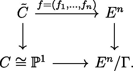
3.1. Discrete invariants
To every such curve we associate discrete invariants as follows. For each we have
Thus we have
Denote
Using the assumption that Pi and Qi are relatively prime and considering contribution of an arbitrary linear form in u, v to various we establish the following:
Note that whenever
and
because otherwise all the four polynomials
have a common divisor.
3.2. Cohomology classes
It is useful to match the discrete invariants M to the homology classes of the strict pullbacks of our curves in where
is the blowup of
in the fixed points of Γ. It is possible to describe this homology group explicitly, but we will not do this. Instead we will think of the homology class of a rational curve as above consisting of two pieces of data:
The homology class of
For each Γ-fixed point
Furthermore, the homology class of in
can be specified by the following data.
Proposition 3.1.
For each curve there exists a unique n × n Hermitian matrix
with entries in
such that for any vector
we have
where Dv is the divisor class given by the pullback of
to En via the map
given by
, and
denotes the conjugate transpose of v.
Proof.
It is well-known that the function is quadratic in v. Thus there exists a unique symmetric
-bilinear form
such that
for all v. But we have
This implies
hence
for any pair of vectors
Let
be the unique
-linear map such that
We have
Since this holds for all the map
must be
-linear. So it can be represented by a matrix with entries in
and that matrix must be Hermitian because the form B was symmetric. □
It is clear that the diagonal entries of are simply the degrees of the components fi of f,
Let us calculate the degree of these components for our construction. Consider the function
This is a rational function of degree b on E because for a generic there are exactly b solutions to
corresponding to the bth roots of
Its pullback to
is the function
Now the equation has
solutions: ck values of u/v obtained by solving
and c/a values of
for each of these. Thus the degree of fi is
A recipe to calculate the off-diagonal entries from the matrices will be given in the next section on a case-by-case basis.
3.3. Calculating k
Finally, we calculate the value of k as a function of n for which we expect to have finite number of our curves passing through a generic point of En. The first coefficient of R(u, v) can be normalized to 1, and we have kc remaining coefficients. A generic point is given by pairs xi, yi satisfying and we can parametrize our curve so that the point
goes to
This fixes the first coefficient of Pi and Qi. Then the condition for a polynomial R to be of the form
is of codimension
Thus the expected dimension of the space of solutions is
We want this number to be equal to 2 because there is a two-dimensional group of translations and rotations acting on solutions that needs to be gauged out. Thus we have
Note that we have in all the three cases, so we obtain
3.4. Summary of the approach
We summarize our strategy for proving rationality of varieties of the form corresponding to triples
and n < c.
Calculate
List possible a×b matrices M and figure out which matrices correspond to which off-diagonal values of H. Obtain a list of possible off-diagonal entries
List possible n×n matrices H up to integral change of basis which are positive-definite, have
For each n×n matrix H list the degrees
For a point
If we are lucky and the answer to the previous step is 1 for a generic point p, then try to construct a vector
4. Example for
In this case the group Γ has order c = 3, so we have only one case n = 2, k = 2. The discrete invariant has the form of a matrix
of non-negative integers with all the row and column sums equal 2. To calculate the 2 × 2 matrix
we already know that the diagonal entries are 2. Let
One can relate to M by the following. Let
be the diagonal. Then we have
Proposition 4.1.
Proof.
Consider curves defined by equations on
(i = 1, 2):
It turns out, that do not intersect. Therefore they have the same homology class. So, by counting the intersection points
Analogously,
The divisor is linearly equivalent to
where D is the divisor at infinity of E, which has degree 3. Thus we obtain
Hence the inequalities are equalities. □
The diagonal corresponds to the vector This gives us
Similarly we obtain the evaluation for the vector which corresponds to the curve
which allows to calculate
Going over the set of possible M we find the set of possible values of
Up to a integral change of basis (a matrix sends H to
) we have two possible matrices, with determinants 3 and 4:
For H3 we have three possible matrices M:
For H4 we have six possible matrices M:
Some matrices do not produce any curves passing through generic points, for instance the first three matrices corresponding to H4. To illustrate our method we give here an explicit parametrization of the curves corresponding to H3:
4.1. H3 curves
It is enough to consider only the first matrix, because the other 2 can be obtained from it by automorphisms:
We want to determine how many curves pass through a given point. Take for i = 1, 2 points on E. If a curve
passes through
then we can choose the coordinates u, v such that p is at v = 0. We can still apply affine transformations
Such a curve is then completely determined by the homogeneous polynomials
of degrees
with first coefficient 1 satisfying the following equations, which follow from
and a similar equation for Q:
In our situation, we have one polynomial of degree 2 and four polynomials of degree 1:
The polynomial of degree 2 is Note that
and
So we can eliminate
from the equations:
The polynomials must be relatively prime, for otherwise
would all share a factor. This implies
Assume Then we uniquely reconstruct
from
Again
are relatively prime, and by applying affine transformations we can move them to an arbitrary pair of distinct linear polynomials with first coefficient 1, for instance u, u – v. So under our assumptions there is at most one curve passing through p. Vice versa, to show that the curve exist we just need to make sure that in our construction the pairs
are relatively prime. This requires another condition:
So we have shown that the curve is unique provided
This means we have to remove the divisors given by vectors (0, 1), (1, 0). Taking any other divisor class we will satisfy conditions for part (i) of Lemma 2.1. To show rationality we need to satisfy the assumptions of part (ii). So we need a divisor with small intersection number with
that is a vector not of the form
whose length is small with respect to the form H. Take
which corresponds to the divisor Dv consisting of
such that
We have
So there is at most 5 points of intersection in
Going down to
we obtain at most
of points of intersection
satisfying
Clearly,
is rational. So the conditions of Lemma 2.1 are satisfied.
4.2. H4 curves
In this case computer experiments showed that there are three curves passing through a generic point for each of the last three matrices M. However these curves can be distinguished by their incidence information with the Γ-fixed points, so probably it is possible to use these curves for an alternative rationality proof.
4.3. Total curve count
In total we obtain three curves for H3 and nine curves for H4. However, these curves can be distinguished by our discrete invariants and by their intersections with
5. Examples for
If we can have n = 2 or n = 3. Here
For n = 2 we obtain k = 1. For n = 3 we obtain k = 2. The matrices
are 2 × 4 with column sums k and row sums 2k. The matrices H have 2k on the diagonal.
Proposition 5.1.
The intersection number of the diagonal and
is given by
Proof.
We have curves given by equations (l = 0, 1,
)
The pairs representing the same homology class are listed as follows So
This is because each root of has multiplicity 4 in
and there are further
points with w = 0 on
which map to the points with
Producing similar inequality for
and adding to the one above we obtain
On the other hand, is equivalent to
where D is the divisor at infinity consisting of two points. So the intersection equals 8k. Therefore our inequalities must be equalities. □
This allows us to compute as a function of the entries of
The diagonal corresponds to the vector
so we have
Hence The vector
corresponds to the curve
so the corresponding intersection number is
We obtain Thus
5.1. The case k = 1, n = 2
There are two H-matrices (up to automorphisms) for n = 2, k = 1, of determinants 2 and 4:
For H2 there is only one matrix M:
For H4 there are two matrices:
It is not so difficult to check that each of the three matrices M leads to a good family of curves.
5.2. The case k = 2, n = 3
With n = 3 the set of possibilities is much bigger. We have 19 possible matrices M. They produce the following list of 13 possible off-diagonal entries for H:
To construct a curve we need to choose three of them to get with
So there are
possibilities. Classifying all the possible positive definite 3 × 3 matrices H up to
action produces 14 cases with determinants
Counting curves on a computer produces .Footnote5
Table 1. Curve counts for n = 3, k = 2.
The H-matrices with 0 curves are the following matrices with determinants 8 resp. 16:
It turns out that nonexistence of these curves is explained by the fact that the matrices can be conjugated to
which contain forbidden off-diagonal entries
Note that for each matrix H there are several triples of matrices The table was obtained by adding the point counts for all triples. In some situations the total number of curves can be greater than 1, but for some individual triples
the number is 1. We will work with the matrix of determinant 16 which gives one curve. The matrix is
The matrices are as follows:
Computer experiments show that exactly one curve passes through a generic point of E3. To apply Lemma 2.1 in full generality we need to choose a divisor. So we look for a vector v whose H-norm is small, but not too small. All vectors of norm 4 do not produce good divisors: through a generic point of such divisor there are no curves of our type. There are no vectors of norms between 4 and 8. There are 252 vectors of norm 8. Let
be the group of matrices
such that
The vectors of norm 8 form 3
-orbits. Some of these vectors are also such that through a generic point of the corresponding divisor there are no curves. In the orbit of
which consists of 192 vectors, for 168 vectorsFootnote6 the curve count is 1 and for the remaining 24 it is 0. This vector produces a divisor
satisfying the conditions of Lemma 2.1. We have
so if we show that at least one intersection point is at infinity, we obtain that the number of finite intersection points of
with C is at most
The points at infinity of Dv are four points out of the total
points at infinity on E3. These are the points
satisfying
The points at infinity are of order 2, so this condition is equivalent to p1 = p3. Let
be the projection of
to E × E using coordinates 1, 3. So it is enough to show that
intersects Δ at infinity. The intersection number is 8, but there are only four finite intersection points because
Thus there must be intersections at infinity.
6. Examples for
Finally, we turn to the most interesting example, which includes open cases. We have and n = 4 or n = 5. Here
For n = 4 we obtain k = 1. For n = 5 we obtain k = 2. The matrices
are 2 × 3 with column sums 2k and row sums 3k. The matrices H have 6k on the diagonal. Some things are simpler because there is only one point at infinity, and the correspondence between M-matrices and the off-diagonal entries of the H-matrix are bijective.
Proposition 6.1.
The intersection number of the diagonal and
is given by
Proof.
We have curves given by equations (l = 0, 1, r = 0, 1, 2)
We have
This is because each root of has multiplicity 6 in
and there are further
points with w = 0 on
which map to the points with
Producing similar inequality for
and adding to the one above we obtain
On the other hand, the divisor of the rational function is
where D is the point at infinity. Therefore
Therefore our inequalities must be equalities. □
This allows us to compute as a function of the entries of
The diagonal corresponds to the vector
so we have
The vector corresponds to the curve
so the corresponding intersection number is
So we can recover
6.1. The case k = 1, n = 4
The diagonal entries of H are 6 and the possible off-diagonal entries are in the set
We classified all matrices H up to -equivalence satisfying the following conditions:
H is positive definite.
There is no vector
For any
It turns out there are five matrices with determinants
Note that the off-diagonal values 0 resp. correspond to
The curve counts are given in .Footnote7 It is not clear why curves corresponding to H864 do not pass through generic points.
Table 2. Curve counts for n = 4, k = 1.
We turn our attention to the matrix which already implies unirationality of X4,6 and will also imply rationality if we find a “good” divisor class. The group
has order 155,520 and acts transitively on the 240 vectors of H-norm 6 and on the 2160 vectors of H-norm 12. Vectors of norm 6 intersect C only at infinity, so we pick a vector of norm 12. Some of the vectors of norm 12 correspond to the “diagonals,” for instance
For this vector we obtained 0 curves. However picking
and any other vector not of the form
for some i, j or a permutation of such, we obtain 1 curve.
Note that for any v of norm 12 and any curve C of our kind the number of intersection points outside of the Γ-fixed points is at most 1. This is true because
and the intersection
contains at least one point at infinity.
So we make the following Conjecture, which by Lemma 2.1 implies rationality of X4,6:
Conjecture 6.2.
For denote by
the number of curves
of our type corresponding to the matrix H144 and containing p. Then for a generic point
we have
Moreover, for a generic point
we have
where
We verified this conjecture by testing the statement on 10,000 random points on and 10,000 random points on E4 over the field
Only 1 point got “unlucky” and the number of curves was 0. For every other point the number was 1. Counting the curves took
s per point on an ordinary laptop.
6.2. The case k = 2, n = 5
Finally we turn to the most interesting case. The diagonal entries of H are 12 and the possible off-diagonal entries are in the set
We could not classify all such matrices H up to -equivalence because the set of possibilities is too big. However the following matrix seems to be the only matrix up to
-equivalence of the smallest possible determinant
We consider Note that the off-diagonal value
resp.
corresponds to
resp.
There are exactly 336 vectors of H-norm 12. Since every curve
has 12 points at infinity, these curves cannot pass through generic points of divisors corresponding to these vectors. Just for reference we mention that the size of the group
is 6912. The vectors of H-norm 12 form three orbits of sizes 48, 192, 96, represented by the basis vectors e1, e3, e5. The next possible H-norm is 18, and there are 768 vectors of norm 18 forming a single
-orbit. For such a vector v we have
and at least 12 points of intersection are at infinity. Therefore
Some vectors represent “generalized diagonals,” for instance
We found that our curves do not pass through generic points on the corresponding divisors. Taking any vector different from those do seem to produce good divisors, for instance we take
The following conjecture implies unirationality of X5,6 by part (i), Lemma 2.1:
Conjecture 6.3.
For denote by
the number of curves
of our type corresponding to the matrix H13824 and containing p. Then for a generic point
we have
The following conjecture together with rationality of X4,6 implies rationality of X5,6 by Lemma 2.1:
Conjecture 6.4.
With defined in Conjecture Citation6.Citation3, for a generic point
we have
where
6.3. Computations for n = 5
The computations in these cases take much more time than in the n = 4 case. It can probably be explained by the fact that the set of divisors where the number of curves is not 1 is huge: for instance, it must contain all divisors Dv corresponding to the 336 vectors v of H-norm 12. Another issue is that when we create the ideal parametrizing our curves, we have besides equations also inequalities of the form
(3)
(3)
Each inequality is imposed by adding an extra variable Ji and an extra equation
(4)
(4)
Note that the degrees of Pi and Qi are 6 and 4 respectively, so the resultant has degree 24 and these extra equations are very long. On the other hand, when we tried to keep only the equations without the inequalities the length of the scheme of solutions grew up to 99. The scheme turned out to contain a single isolated point and several very fat points failing the conditions
The computation with the inequalities Equation(3)(3)
(3) takes ≈ 1 hour 15 min on an ordinary laptop (for each random point on E5). It turns out, it is better to extend the set of inequalities that translate to EquationEquation (4)
(4)
(4) by a much larger set of 32 inequalities
(5)
(5)
For each inequality we have to create a new variable and a new equation as in Equation(4)(4)
(4) . These inequalities formally follow from Equation(3)
(3)
(3) as explained in Section 3.1, but their degrees are much smaller. On the other hand, inequalities 5 do not seem to imply 3. Thus we must additionally test that every solution we find satisfies 3.
It turns out, that it is faster to build the ideal step-by-step. On each step we add some new equations and recompute the Gröbner basis. In the very beginning we choose a cell of the cell decomposition of the weighted projective space we do computations in. The total number of variables is 120 (we have 10 pairs and for each pair i, j we have six polynomials
whose degrees are given by the entries of
). Among these variables 42 have weight 1, 38 have weight 2, 22 have weight 3, and 18 have weight 4. We order the variables by weight, and if the weights agree by the degree of the polynomial they are coefficients of. Because we should consider the solutions up to translation, we set the very first variable to 0. The choice of a cell in the weighted projective space means we set the first r variables to 0, the r + 1st variable to 1. We need to do this for every r,
Then we have three steps (for each r):
Add equations coming from elimination of Pi, Qi from the main EquationEquation (2)
Add variables and equations representing EquationEquation (5)
Add variables and equations representing EquationEquation (3)
Then we compute the dimension over the base field of the quotient ring with respect to the ideal obtained in the final step. This number divided by the weight of the variable we made equal to 1 is the number of points in the given cell. If after some step we obtain the ideal EquationEquation (1)(1)
(1) , this means there are no solutions in a given cell, so we abort and pass to the next cell, that is next value of r. In all situations we encountered, all the solutions belonged to the biggest cell.
Complete computation for each point takes
min on an ordinary laptop. Initially, we made 10 trials for each of the Conjectures Citation6.Citation3, Citation6.Citation4, and obtained exactly 1 curve in all cases. The referee suggested that a more extensive testing would provide more evidence for the conjectures, so we ran 10,000 trials for each of the Conjectures Citation6.Citation3, Citation6.Citation4 on a cluster (200 cores,
h). We found two failures of Conjecture Citation6.Citation3 and one failure of Conjecture Citation6.Citation4, which we believe is a convincing evidence, see Section 2.1. The source code and the output logs are available online at https://mellit.xyz/post/rationality/.
Remark 6.1.
The quadratic form induced by H13,824 on the rank 10 lattice is proportional to the so-called laminated lattice
see [Citation5]. We discovered this fact with the help of OEIS ([Citation7], sequence A006909) by searching for the sequence of numbers of vectors of given norm, which begins as follows:
In fact, the matrix H144 from Section 6.1 in a similar way corresponds to the lattice E8. The matrix H16 from Section 5.2 corresponds to the lattice D6.
Acknowledgments
I would like to thank F. Catanese for giving a wonderful talk about Ueno-Campana varieties, and K. Oguiso for a stimulating discussion and encouragement. I thank G. Williamson for correcting the statement of Corollary 1.3. Initial results of this work were obtained in 2014 during my stay at ICTP, Trieste. The work was completed in 2017 during my stay at IST Austria. I performed extensive testing of Conjectures Citation6.Citation3, Citation6.Citation4 during my visit to ICTP in 2019. I am grateful to ICTP for hospitality and for providing me with the computational resources of the cluster ARGO.
Declaration of Interest
No potential conflict of interest was reported by the author.
Additional information
Funding
Notes
1 We include the case c = 3 for completeness and because it helps to illustrate our techniques.
2 In our computations we used SAGE [Citation11], which delegates Gröbner basis computations to Singular [Citation6] and certain lattice algorithms to GAP [Citation8].
3 We thank the anonymous referee for this observation.
4 The only cases with n > 1 when this number is not an integer are with n = 2, 3. In these cases the method can still be applied. The curve
should pass through Γ-fixed points of orders different from 6, which implies a slightly different general shape of the EquationEquation (1)
(1)
(1) . We do not include these situations here because it would complicate the notations, and because these cases are already known to be rational anyway.
5 The values in the table are conjectural, they were obtained by testing on random points over the finite field see Section 2.1. We used exactly the same computer program as for testing Conjectures Citation6.Citation2, Citation6.Citation3, Citation6.Citation4 below.
6 Elements of acting on E3 do not change H, but they still permute the 8 points at infinity. So the true symmetry group of the system is not
but a certain congruence subgroup. This explains why we obtain different curve counts for vectors of the same
-orbit.
7 Similarly to , the values in are conjectural, they were obtained by testing on random points over the finite field , see Section 2.1. The same computer program was used.
References
- Campana, F. (2011). Remarks on an Example of K. Ueno, Classification of Algebraic Varieties. Based on the Conference on Classification of Varieties, Schiermonnikoog, Netherlands, May 2009. Zürich: European Mathematical Society (EMS), pp. 115–121.
- Catanese, F., Oguiso, K, Truong, T. T. (2014). Unirationality of Ueno-Campana’s threefold. Manuscr. Math. 145(3–4): 399–406. doi:10.1007/s00229-014-0680-z
- Catanese, F., Oguiso, K, Verra, A. (2015). On the unirationality of higher dimensional Ueno-type manifolds. Rev. Roum. Math. Pures Appl. 60(3): 337–353.
- Colliot-Thélène, J.-L. (2015). Rationalité d’un fibré en coniques. Manuscr. Math. 147(3–4): 305–310. doi:10.1007/s00229-015-0758-2
- Conway, J. H, Sloane, N. J. A. (1993). Sphere Packings, Lattices, and Groups, Grundlehren der Mathematischen Wissenschaften, 290. Springer-Verlag, New York.
- Decker, W., Greuel, G.-M., Pfister, G, Schönemann, H. (2016). Singular 3-1-7—A computer algebra system for polynomial computations. Available at: http://www.singular.uni-kl.de
- Ionescu, P, Naie, D. (2003). Rationality properties of manifolds containing quasi-lines. Int. J. Math. 14(10): 1053–1080. doi:10.1142/S0129167X03002095
- Oguiso, K, Truong, T. T. (2015). Explicit examples of rational and Calabi-Yau threefolds with primitive automorphisms of positive entropy. J. Math. Sci. Univ. Tokyo. 22(1): 361–385.
- The GAP Group. (2016). GAP – Groups, Algorithms, and Programming, Version 4.8.3. Available at: https://www.gap-system.org
- The On-Line Encyclopedia of Integer Sequences. (2017). Available at: https://oeis.org
- The Sage Developers, Sagemath, The Sage Mathematics Software System. (2016). Version 7.3. Available at: http://www.sagemath.org
- Ueno, K. (1975). Classification Theory of Algebraic Varieties and Compact Complex Spaces, Lecture Notes in Mathematics Vol. 439. Springer-Verlag, Berlin-New York.