Numerical Simulations and Design Optimization of Compressor Cascade Flow Using One Equation and Wray-Agarwal Turbulence Model

Abstract

The unsteady simulations are conducted, and the computed results with WA model are compared with the experimental data in conjunction with the simulation results obtained using traditional models. It is shown that on the mid-span sections of the cascade airfoils the distributions of near-wall static pressure coefficients from each turbulence model agree well with the experimental data. On the lower spanwise sections, the discrepancy between the numerical simulations and experimental data generally increases. Among the three turbulence models, the WA turbulence model shows better agreement with the experimental data in predicting the spanwise total pressure losses downstream of the cascade blade. The WA model is then embedded into the adjoint optimisation loop to test its capability in minimising the flow losses in the compressor cascade passage. The optimisation results show that the total pressure loss coefficient of the optimised compressor cascade is reduced by 18.1% compared to the baseline design.

KEYWORDS:

• Turbulence models
• aerodynamics
• URANS
• gas turbine
• design optimisation

1. Introduction

Computational Fluid Dynamics (CFD) has been playing an increasingly important role in the aerodynamic design of gas turbines for past several decades. The inviscid two-dimensional (2D) blade-to-blade and through-flow calculations methods were developed and then widely used in the 1960s; (Hawthorne and Novak 1969) the three-dimensional (3D) inviscid Euler codes were programmed in the 1970s; (Denton 1975) the 3D Reynolds-Averaged Navier-Stokes (RANS) solutions of gas turbine flow field began to appear in the 1980s and the 3D Unsteady Reynolds-Averaged Navier-Stokes (URANS) simulations were first conducted in the 1990s (Dawes 1988; Chen and Whitfield 1993). Nowadays, advanced compressor or turbine designs would be unimaginable without the aid of CFD.

The most complex phenomenon inside turbomachines is the turbulent nature of the flow, and the CFD prediction of turbulence is a nontrivial problem in the aerodynamic design of gas turbines. Recently, although Direct Numerical Simulation (DNS) solutions have begun to appear in fundamental research projects, they are still too expensive for routine predictions of turbulent flow in engineering designs. A more practical approach is to employ the Reynolds- Averaged Navier-Stokes (RANS) equations in conjunction with various turbulence models (Bradshaw 1996). Thus, the CFD technology based on RANS/URANS simulations in conjunction with turbulence models has been widely used in the design process of industrial compressors or turbines (Everitt and Spakovszky 2013; Montomoli, Hodson, and Lapworth 2011; Schobeiri and Abdelfattah 2013).

In many of these turbulence models, the eddy viscosity assumption called the Boussinesq hypothesis, is made to relate the turbulent stresses to the mean flow by solving an additional algebraic (zero) equation (Chen and Xu 1998) or one partial differential equation (PDE) for a turbulence variable (Spalart and Steven 1992) or two PDEs for transport of two variables defining the turbulence (Menter 1992), (Pope and Stephen 2000). At present, the two-equation k-ω Shear Stress Transport (SST) turbulence model is widely used in simulating the internal flow inside the gas turbine. The SST model generally shows satisfactory prediction at the design points of the fluid machinery; however, the simulation results normally have significant deviations from the experimental data under the off-design operating conditions. In the literature, higher-order correlations for turbulent variables have been suggested to improve the prediction accuracy but they usually result in models with more transport equations such as the full Reynolds Stress Model (RSM) resulting in six equations that require more computational cost.

Since the key turbulence information has been included in the one-equation turbulence models; they can be considered as a good compromise between the zero-equation model and the two-equation model giving both accurate (acceptable accuracy in a large number of industrial applications) and computationally efficient results. The one-equation Spalart-Allmaras (SA) model which is widely used in the aerospace industry has achieved a great deal of success in the prediction of wall-bounded flows. However, the SA model has been shown to produce errors in some free shear flows because of the single-equation formulation of SA model has limitations in accurately predicting the turbulence length and time scales (Fares and Schröder 2005).in free shear flows. Therefore, the focus of this paper is on the application of a recently developed more accurate and cost-efficient one-equation turbulence model for solving the complex gas turbine flow. The innovative one-equation Wray-Agarwal (WA) turbulence model was recently developed by Wray and Agarwal at the CFD Lab at Washington University in St. Louis (Wray and Agarwal 2015). The WA model is derived from the k-ω closure, and has an obvious distinction with the previous k-ω based models. In the WA model, the cross-diffusion term is included in the ω equation, and a blending function is employed to control the cross-diffusion term.

To date, the WA model has shown a great deal of promise in accurately and efficiently simulating a wide range of complex flows. It is found that the WA model is more accurate than the traditional one-equation SA model and more efficient than the k-ω SST model for a large number of benchmark flows. (Wray 2016) Han et al. (2015) calculated the 3D S-duct flow using the WA model and their conclusions showed that the WA model matched the experimental data better compared to the SA and k-ω SST model. Yi et al. (2019) simulated the multiphase flow based on the WA model and concluded that the WA turbulence model shows better accuracy and computational efficiency when compared to the traditional two-equation turbulence models. Furthermore, Ji et al. (2021) used the WA model to simulate the 3D centrifugal pump flow and the results showed that the WA model gave a higher prediction accuracy than the other one- and two-equation turbulence models.

The wide range of WA model applications for many canonical flows from the National Aeronautics and Space Administration (NASA) Turbulence Modeling Resource (TMR) (more details can be found on the official website: https://turbmodels.larc.nasa.gov/wray_agarwal.html) also provide us confidence in applying it to more complex flow fields. Until now, the prediction capability of the WA turbulence model hasn’t been verified for simulating gas turbine flows. Thus, in this paper, the WA turbulence model is employed to investigate the 3D compressor cascade flow under different incidence angles, and the simulation results of the near-wall pressure coefficients, downstream total pressure loss coefficients, etc., are compared to the experimental data as well as with the CFD results obtained using the SA model and k-ω SST model. Additionally, the Detached-eddy simulation (DES) version of the WA model is used to calculate the flow field which shows improvements in results compared to those obtained with standard WA model. Next, the aerodynamic shape of the compressor cascade is then optimised to reduce the flow losses by employing the adjoint optimisation algorithm in conjunction with the WA-DES turbulence model results. The aim of conducting the adjoint optimisation here is to test the performance of the WA model in the gradient-based optimum-searching process. The flow mechanisms that lead to the performance improvement in optimised cascade are then discussed through post-processing of the WA model results.

2. Wray-Agarwal (WA) Turbulence Model

The WA model has gone through a couple of versions (Han, Rahman, and Agarwal 2018), and here the latest version (WA 2017) is used to conduct the numerical simulations. The key feature of the model is the switching function $f_1$ which allows the model to behave like $k-\omega$ closure near the wall and as $k-\epsilon$ closure in the far field. The WA model solves the variable $R$ ($R=k/\omega$) based on the equation below: (1) $\begin{array}{rl}\frac{\mathrm{\partial }R}{\mathrm{\partial }t}+\frac{\mathrm{\partial }{u}_{j}R}{\mathrm{\partial }{x}_j}& =\frac{\mathrm{\partial }}{\mathrm{\partial }{x}_j}\left[({\sigma }_{R}R+\nu )\frac{\mathrm{\partial }R}{\mathrm{\partial }{x}_j}\right]+C_{1}RS\\ & +f_1{C}_{2k\omega }\frac{R}{S}\frac{\mathrm{\partial }R}{\mathrm{\partial }{x}_j}\frac{\mathrm{\partial }S}{\mathrm{\partial }{x}_j}-(1-f_1)min\\ & \times \left(C_{2k\epsilon }{R}^2\left(\frac{\frac{\mathrm{\partial }S}{\mathrm{\partial }{x}_j}\frac{\mathrm{\partial }S}{\mathrm{\partial }{x}_j}}{S^2}\right)\text{, }{C}_m\frac{\mathrm{\partial }R}{\mathrm{\partial }{x}_j}\frac{\mathrm{\partial }R}{\mathrm{\partial }{x}_j}\right)\end{array}$(1) The turbulent eddy viscosity ${\mu }_t$ is calculated by: (2) ${\mu }_t=\rho f_{\mu }R$(2) where $\rho$ is the flow density. $S$ is the mean strain given by: (3) $\begin{array}{rl}S& =\sqrt{2S_{ij}{S}_{ij}}\end{array}$(3) (4) $\begin{array}{rl}{S}_{ij}& =\frac{1}{2}\left(\frac{\mathrm{\partial }{u}_i}{\mathrm{\partial }{x}_j}+\frac{\mathrm{\partial }{u}_j}{\mathrm{\partial }{x}_i}\right)\end{array}$(4) Here the authors used $S=\text{max}(S,{10}^{-16}{s}^{-1})$ to avoid division by zero value. The damping function $f_{\mu }$ is deployed in the model to account for the wall-blocking effect: (5) $\begin{array}{rl}{f}_{\mu }& =\frac{{\chi }^3}{{\chi }^3+C_{\omega }^3}\end{array}$(5) (6) $\begin{array}{rl}\chi & =\frac{R}{\nu }\end{array}$(6) (7) $\begin{array}{rl}\nu & =\frac{\mu }{\rho }\end{array}$(7)

The value of coefficient $C_{\omega }$ is listed in Table 1. The function $f_1$ was built to allow the WA model to switch between two destruction terms: (8) $\begin{array}{rl}{f}_1& =min(\tanh (ar{g}_1^4),0.9)\end{array}$(8) (9) $\begin{array}{rl}ar{g}_1& =\frac{1+\frac{d\sqrt{RS}}{\nu }}{1+{\left[\frac{max\left(d\sqrt{RS},1.5R\right)}{20\nu }\right]}^2}\end{array}$(9) where $d$ is the minimum distance to the nearest wall surface. The value of R is zero on the solid walls, and R is set to be 4 times the freestream kinematic viscosity at the inlet boundary. Various constants used in the WA model are given in Table 1.

3. Computational Setup

3.1. Reference Compressor Cascade Geometry

The NACA-65 profile-based linear compressor cascade is selected as the reference geometry. The well-documented experimental measurements of this ?>cascade row have been reported by Ma (2012), (Gao et al. 2015) at École Centrale de Lyon. The key design parameters of the compressor cascade are shown in Table 2.

Table 1. Constants used in WA turbulence model.

Constant Symbols	Value
$C_{1k\omega }$	0.0829
$C_{1kϵ}$	0.1127
$C_1$	$f_1(C_{1k\omega }-C_{1kϵ})+C_{1kϵ}$
${\sigma }_{k\omega }$	0.72
${\sigma }_{kϵ}$	1.0
${\sigma }_R$	$f_1({\sigma }_{k\omega }-{\sigma }_{kϵ})+{\sigma }_{kϵ}$
$C_{2k\omega }$	${\displaystyle \frac{C_{1k\omega }}{{\kappa }^2}}+{\sigma }_{k\omega }$
$C_{2kϵ}$	${\displaystyle \frac{C_{1kϵ}}{{\kappa }^2}}+{\sigma }_{k\omega }$
$\kappa$	0.41
$C_{\omega }$	8.54

Table 2. Key parameters of compressor cascade.

Parameter	Value
Chord length	150.00 mm
Span length	370.00 mm
Solidity	1.12
Stagger angle	42.70°
Camber angle	23.22°
Aspect ratio	2.47
Design upstream flow angle	54.31°
Design downstream flow angle	31.09°
Inlet velocity magnitude	40.00 m/s

3.2. Numerical Scheme and Grid Generation

In this study, the 3D URANS equations are solved to simulate the compressor cascade flow. The reason for conducting unsteady simulations is that there are obvious flow separations inside the compressor cascade passage especially when the incidence angle becomes a large value, and the URANS should be a more suitable approach in solving the large-separation flows than the steady RANS. The pressure-velocity coupling scheme is deployed to update the flow pressure and velocity simultaneously in each calculation step. For the spatial discretization, the finite volume method with second-order upwind scheme is used for the convection terms in the governing URANS equations. The second-order central difference scheme is employed for the diffusion terms. The implicit scheme is employed for temporal discretization.

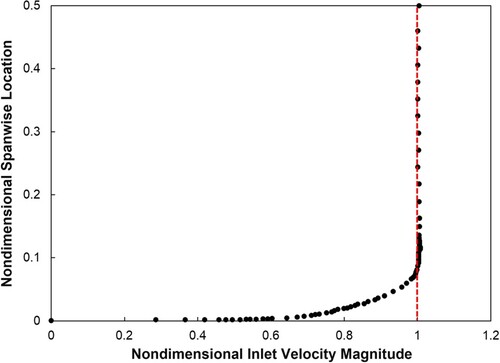
The computational domain and boundary conditions are set as shown in Figure 1. The computation domain is extended 2.9 and 3.7 times axial chord length upstream and downstream of the compressor cascade, respectively. It should be noted that there is no tip clearance inside the cascade passage domain. The inlet velocity components and outlet static pressure values are specified on the inlet and outlet planes, respectively. The total temperature is set to 288.15 K. The circumferentially averaged mean fully turbulent inlet velocity profile measured by the hot-wire anemometry in experiment (Ma et al. 2013) (as shown in Figure 2) is employed to make the simulations consistent with the actual experimental conditions as much as possible. As a result, the chord length-based Reynold number is $3.82\times {10}^5$. The constant static pressure is specified to be 101325 Pa on the outlet section, and the fluid medium is considered incompressible air (density is 1.225 $kg/m^3$). The half-span cascade passage domain is simulated here by using the symmetric plane to reduce the computational cost, and the translational periodic boundary condition is employed on the lateral surfaces of the computational domain. The non-slip wall condition is set on the compressor cascade and end wall surfaces.

Figure 1. Computational domain and boundary conditions of compressor cascade.

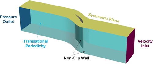
Figure 2. Inlet velocity profile in computational domain.

The mesh in the passage was generated using the commercial software package ANSYS/ICEM-CFD. The H-O-H topology was deployed to spatially discretize the cascade passage domain and the O-type mesh was generated near the cascade wall. The height of the first layer cell near the wall surface is set to be 2e-5 m to guarantee that the value of $y^{+}$ is close to 1 inside the entire computational domain. Five sets of meshes are used for grid independence of the solution study with the number of grid points of 1, 1.5, 2, 2.5, 3 and 5 million, respectively. Here the total pressure loss coefficient $\zeta$ is chosen as an aerodynamic performance indicator, and its definition is as follows: (10) $\zeta =(P_{t\mathrm{\_}inlet}-P_{t\mathrm{\_}outlet})/(P_{t\mathrm{\_}inlet}-p_{s\mathrm{\_}inlet})$(10) where $P_{t\mathrm{\_}inlet}$ represents the inlet total pressure, $P_{t\mathrm{\_}outlet}$ the outlet total pressure and $p_{s\mathrm{\_}inlet}$ the inlet static pressure.

Numerical summations for five flow passing cycles (i.e. the computation domain length divided by the axial velocity magnitude) are initially needed before the flow shows a periodic behaviour, and the time-averaged physical quantities are then sampled. Here the adaptive time step is set to keep the Courant number value around 1. In addition, the inner-loop calculations are regarded as convergent when the maximal residual value becomes smaller than 1e-6. The relative change in the total pressure loss coefficient (at an incidence angle of 4 degrees) with an increase in the number of grids is shown in Figure 3. This figure shows that the variation in the total pressure loss coefficient becomes negligible when the mesh has larger than 2.5 million grid points. To further investigate the convergence of solution independent of cascade passage grids, the Richardson extrapolation method (details given on the NPARC Alliance CFD Verification and Validation Website https://www.grc.nasa.gov/www/wind/valid/tutorial/spatconv.html) is employed for estimating the prediction error with various meshes. The basic idea of Richardson extrapolation is based on the Taylor series representation and can deliver a higher-order estimate of continuum value from the series of lower-order discrete values. Here the Richardson extrapolation is assumed to provide a fourth-order estimate of the continuum value (i.e. the total pressure loss coefficient at ideal zero grid spacing). The estimated fractional error $\epsilon$ for different meshes is defined as follows: (11) $\epsilon =\frac{{\zeta }_{fine}-{\zeta }_{ref}}{{\zeta }_{ref}}$(11) where ${\zeta }_{ref}$ refers to the total pressure loss coefficient with a mesh number of 1 million, and ${\zeta }_{fine}$ represents the CFD solution with a finer mesh. 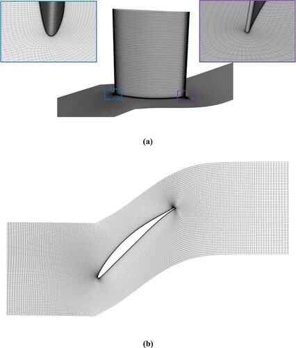The computed distributions of the estimated fractional error $\epsilon$ with the variable number of computational meshes are also shown in Figure 3. The error prediction results based on Richardson extrapolation show the asymptotic tendency when the grid number is larger than 2.5 million. Based on the comprehensive consideration of simulation accuracy and calculation cost, the mesh with 2.5 million grid points is finally chosen in the following simulations. The detailed two-dimensional (2D) and 3D mesh inside the compressor cascade passage are shown in Figure 4.

Figure 3. Study of mesh size on solution and relative error.

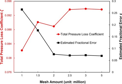
Figure 4. Mesh generated inside the compressor cascade passage (2.5 Million): (a) 3D passage mesh, (b) 2D cascade mesh.

4. Simulations Results

4.1. Incidence Angle of 0 Degree

The compressor cascade flow is first simulated at an incidence angle of 0 degree, and the three turbulence models namely WA, SA and $k-\omega$ SST are employed. The simulation results of the near-wall static pressure coefficients $C_p$ on two span-wise cross-sections are then compared to the experimental data. The definition of $C_p$ is: (12) $C_p=\frac{p_{s\mathrm{\_}nearwall}-p_{s\mathrm{\_}inlet}}{P_{t\mathrm{\_}inlet}-p_{s\mathrm{\_}inlet}}$(12) where $p_{s\mathrm{\_}nearwall}$ represents the time-averaged near-wall static pressure at the measurement points. 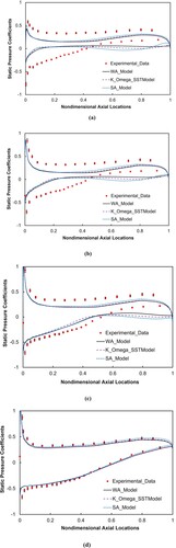Assuming that the relative error or uncertainty in the experimental data is 5%, the detailed comparison of computed $C_p$ with experiment is shown in Figure 5. It shows that the simulation results obtained from all three turbulence models agree well with the experimental data at the 50% span-wise section, which can be expected since there is no obvious flow separation in the mid-span region at an incidence angle of 0 degree. In this case, the cascade span is long enough that the end-wall flow effect on the midspan flow is negligible. Some deviations exist between the experimental data and the simulation results in the near-wall static pressure coefficients at the 5.4% span-wise section. This phenomenon occurs because the cascade flow becomes complex at these lower-span sections when the cascade boundary layer flow merges with the end-wall boundary layer flow in this region. In summary, the horse-shoe vortices, passage vortices and corner separation vortices are generated simultaneously near the end-wall region, which substantially increases the spatial–temporal complexity of cascade passage flow.

Figure 5. Near-wall static pressure coefficients at two different span-wise stations at incidence angle of 0 degree at (a) 5.4% span-wise station, and (b) 50% span-wise station (mid-span).

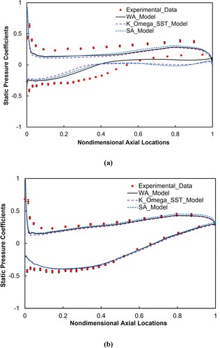
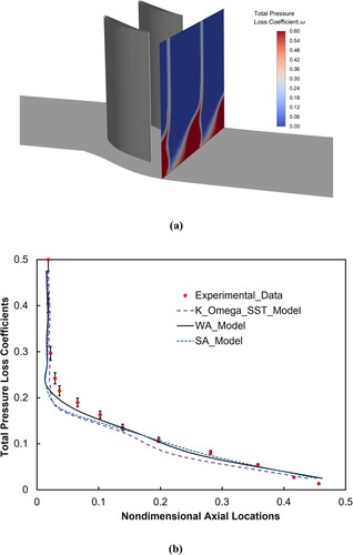
Although the prediction capability of URANS simulations becomes weak in simulating these significant 3D flow separations at the lower-span sections, the WA model shows an improved performance in predicting the near-wall static pressure on the rear part of the cascade suction surface compared to the SA model and $k-\omega$ SST model. Apart from the near-wall static pressure coefficients, the flow losses downstream of the compressor cascade are also calculated and compared to the experimental data. Here the contours of the total pressure loss coefficients predicted by the WA turbulence model on the downstream plane surface (36.3% axial chord length downstream of the cascade trailing edge) in conjunction with the comparison of the circumferentially averaged total pressure loss coefficients are shown in Figure 6. Here the relative error or uncertainty in experimental data is set to be 5%. It shows that the 3D corner separation flow generates the bulk of high aerodynamic losses near the end-wall region, and this phenomenon can be predicted by the WA turbulence model. As for the span-wise distributions of the circumferentially averaged total pressure loss coefficients, the WA model shows a comparable performance when compared to the SA and $k-\omega$ SST models.

Figure 6. Total pressure loss coefficients downstream of compressor cascade at incidence angle of 0 degree: (a) contours of total pressure loss coefficient downstream of compressor cascade, and (b) span-wise distributions of circumferentially averaged total pressure loss coefficients.

4.2. Incidence Angle of 2 Degree

The URANS simulations at an incidence angle of 2 degree are then conducted using the abovementioned three turbulence models. Assuming the relative error or uncertainty in experimental data is 5%, the comparison of the computed near-wall static pressure coefficients $C_p$ with experiment at two different span-wise cross-sections is shown in Figure 7. Similar to the simulation results at the incidence angle of 0 degree, the prediction results obtained using either the SA model or WA model agree well with the experimental data at the 50% span-wise section while some deviations between simulation results and experimental data can be observed at the 5.4% span-wise section. The premature boundary layer flow separation (noted by the plateau in the static pressure coefficient curve) on the cascade suction surface is predicted by all three turbulence models. This is also due to the intrinsic flaw in the RANS approaches in modelling the large-size separated flows.

Figure 7. Near-wall static pressure coefficients at two different span-wise sections at incidence angle of 2 degrees at (a) 5.4% span-wise section, and (b) 50% span-wise section.

The contours of the total pressure loss coefficients predicted by the WA turbulence model on the downstream plane surface (36.3% chord length downstream of cascade trailing edge) in conjunction with the comparison of circumferentially averaged total pressure loss coefficients are shown in Figure 8. Here the relative error or uncertainty in experimental data is set to be 5%. Compared to the compressor cascade flow at the incidence angle of 0 degree, the downstream aerodynamic losses near the end-wall are increased because of the enlarged corner separation at a larger incidence angle of 2 degree. Based on the knowledge of turbomachinery aerodynamics, the horse-shoe vortices, passage vortices and corner separation vortices become stronger inside cascade passage when the larger boundary layer separation is induced by the more obvious flow deceleration effect and the resulting larger adverse pressure gradient. Here the WA turbulence model shows a better prediction capability in simulating the end-wall flow losses compared to the other two turbulence models.

Figure 8. Total pressure loss coefficients downstream of compressor cascade at incidence angle of 2 degrees: (a) contours of total pressure loss coefficient downstream of cascade, and (b) span-wise distributions of circumferentially averaged total pressure loss coefficients.

4.3. Incidence Angle of 4 Degrees

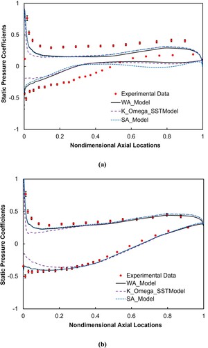
The cascade flow simulations at a larger incidence angle of 4 degree are then conducted. Different from the other two simulations mentioned above, the near-wall static pressure coefficients on two additional span-wise sections (i.e. 16.2% and 1.4% span-wise sections) are available from the experiments and are compared to the numerical simulation results. Assuming that the uncertainty in experimental data is 5%, the corresponding comparison results between experiment and computations are shown in Figure 9. At the 50% span-wise section, the WA turbulence model results are similar to the simulation results obtained from the SA and $k-\omega$ SST models, and all results show good agreement with the experimental data. The discrepancy between the numerical results and experimental data appears when approaching the end-wall sections. Furthermore, the ‘flat region’ of the near-wall static pressure coefficient curve becomes larger and moves upstream when the experimental measurement location moves closer to the end-wall, which is due to the enlarged boundary layer flow separation on the cascade suction surface. Also, the comparison of results shows that all three turbulence models overestimate the flow separations near the end-wall, which is due to the premature suction surface boundary layer flow predicted by the numerical simulations.

Figure 9. Near-wall pressure coefficients at four different span-wise sections at incidence angle of 4 degree at (a) 1.4% span-wise section, (b) 5.4% span-wise section, (c) 16.2% span-wise section, and (d) 50% span-wise section coefficients.

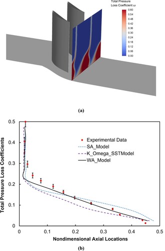
The contours of the total pressure loss coefficients predicted by the WA turbulence model on the downstream plane surface (36.3% chord length downstream of cascade trailing edge) in conjunction with the comparison of circumferentially averaged total pressure loss coefficients at an incidence angle of 4 degree are shown in Figure 10. The contour plot depicts that the corner separation is further strengthened when the incidence angle is increased from 2 degree to 4 degree. The span-wise distributions of total pressure loss coefficients show that the discrepancy between the URANS results and the experimental data (the uncertainty in experimental data is set to be 5%) appears to be below the span-wise 20% cross-section. The simulated flow losses inside the cascade passage are overestimated when compared to the experimentally measured data, which is consistent with the conclusions of the near-wall static pressure coefficients mentioned above. Although the prediction capability of current turbulence models becomes weak in the end-wall region, especially under the inlet boundary condition of a large incidence angle, the WA model shows an enhanced performance when compared to the SA and k-ω SST turbulence models.

Figure 10. Total pressure loss coefficients downstream of compressor cascade at incidence angle of 4 degrees (a) contours of total pressure loss coefficient downstream cascade, and (b) distributions of circumferentially averaged total pressure loss coefficients.

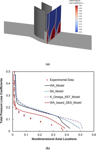
Theoretically, the wide range of length scales should be resolved inside the cascade passage flow if further accuracy improvement of numerical simulations is needed. Due to the limitation of paper length, only one WA model-based detached eddy simulation (DES) is conducted here to verify the potential capability of the WA model after coupling with the DES methodology. More simulations based on the SA-DES and SST-DES will be conducted in the future. DES can be regarded as a hybrid turbulence modelling method combining the Large Eddy Simulation (LES) with the URANS simulations. The WA model predicts the boundary layer flow where LES has high computation cost, and the LES solves the rest of the passage flow, especially the separation flow detached from the wall surface. The DES version of the WA model is shown below: (13) $\begin{array}{rl}\frac{\mathrm{\partial }R}{\mathrm{\partial }t}+\frac{\mathrm{\partial }{u}_{j}R}{\mathrm{\partial }{x}_j}& =\frac{\mathrm{\partial }}{\mathrm{\partial }{x}_j}\left[({\sigma }_{R}R+\nu )\frac{\mathrm{\partial }R}{\mathrm{\partial }{x}_j}\right]+C_{1}RS\\ & +f_1{C}_{2k\omega }\frac{R}{F_{DES}^{2}S}\frac{\mathrm{\partial }R}{\mathrm{\partial }{x}_j}\frac{\mathrm{\partial }S}{\mathrm{\partial }{x}_j}\\ & -(1-f_1)\frac{1}{F_{DES}^2}min\\ & \times \left(C_{2k\epsilon }{R}^2\left(\frac{\frac{\mathrm{\partial }S}{\mathrm{\partial }{x}_j}\frac{\mathrm{\partial }S}{\mathrm{\partial }{x}_j}}{S^2}\right)\text{, }{C}_m\frac{\mathrm{\partial }R}{\mathrm{\partial }{x}_j}\frac{\mathrm{\partial }R}{\mathrm{\partial }{x}_j}\right)\end{array}$(13) where $F_{DES}$ is a function of the ratio between the RANS characteristic length scale $l_{RANS}$ and LES characteristic length scale $l_{LES}$, and can be formulated as: (14) $\begin{array}{rl}{F}_{DES}& =\text{max}\left(\frac{l_{RANS}}{l_{LES}},1\right)\end{array}$(14) (15) $\begin{array}{rl}{l}_{RANS}& =\sqrt{\frac{R}{S}}\end{array}$(15) (16) $\begin{array}{rl}{l}_{LES}& =C_{DES}\text{max}({\mathrm{\Delta }}_x,{\mathrm{\Delta }}_y,{\mathrm{\Delta }}_z)\end{array}$(16)

Here, the value of $C_{DES}$ was calibrated based on the Decaying Isotropic Turbulence (DIT) test, and the value of 0.41 was found to be suitable (Han, Wray, and Agarwal 2017). The boundary conditions and mesh used by DES is kept the same as in the previous numerical setups. Simulations for the first five flow-passing cycles are needed before sampling the instantaneous physical quantities. The Courant number value remains near 1 during the simulation process, and the inner-loop calculations are regarded as converged when the maximum residual value is less than 1e-6. The spanwise distributions of circumferentially averaged total pressure loss coefficients predicted from the WA-based DES model at the incidence angle of 4 degree are then added in Figure 10(b). The results show that WA-based DES results move closer to the experimental data and show superior capability in predicting the large separation flow when compared to the other traditional turbulence models. This also proves that the turbulence model with resolutions at different length scales is necessary for the high-fidelity simulations of gas turbine flow.

5. Design Optimization

The adjoint optimisation is conducted to test the performance of the WA model in the automatic optimisation loops for minimising the aerodynamic loss inside the cascade passage. Here the incidence angle is fixed at 4 degree without loss of generality. The basic idea of adjoint optimisation is to obtain the gradient information of the objective function to the inlet design variables by solving an additional adjoint equation. The objective function $I$ is assumed to be a function of the flow variable $U$ and the design variable $\alpha$: (17) $I=I(U,\alpha )$(17) The CFD governing equations can be simplified to: (18) $G(U,\alpha )=0$(18)

Thus, the gradient of the objective function to the design variables is given by: (19) $\frac{dI}{d\alpha }=\frac{\mathrm{\partial }I}{\mathrm{\partial }\alpha }+\frac{\mathrm{\partial }I}{\mathrm{\partial }U}\frac{\mathrm{\partial }U}{\mathrm{\partial }\alpha }$(19) Generally, the calculation of the term $\frac{\mathrm{\partial }U}{\mathrm{\partial }\alpha }$ needs the solution of the 3D governing equations at each time of change in the design variable $\alpha$, which makes the whole optimisation process computationally expensive. To reduce the computational costs of solving the governing equations, a Lagrange factor $\lambda$ is introduced to form the adjoint equation: (20) $\frac{\mathrm{\partial }I}{\mathrm{\partial }U}+{\lambda }^T\frac{\mathrm{\partial }G}{\mathrm{\partial }U}=0$(20)

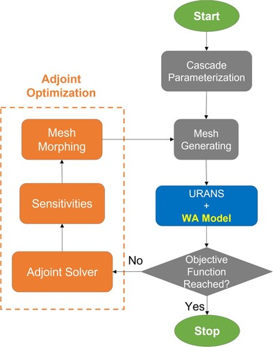
As a result, the gradient of the objective function to the design variables can be obtained by solving the equation: (21) $\frac{dI}{d\alpha }=\frac{\mathrm{\partial }I}{\mathrm{\partial }\alpha }-{\lambda }^T\frac{\mathrm{\partial }G}{\mathrm{\partial }\alpha }$(21) In this study, the discrete adjoint equations based on the discretized form of the governing equations are solved because the discrete adjoint formulation results are much more tightly tied to the numerical implementation of the CFD simulations. More details of the adjoint algorithm in conjunction with the comparison between the discrete adjoint optimisation and continuous adjoint optimisation can be found in the research publication (Li and Zheng 2017). A frozen turbulence assumption that the effect of changes in turbulence is not taken into account when calculating sensitivities was made here. The detailed discrete governing and adjoint equations are added in the Appendix A, and the optimisation flowchart for the compressor cascade flow is shown in Figure 11.

Figure 11. Flowchart of adjoint optimisation process.

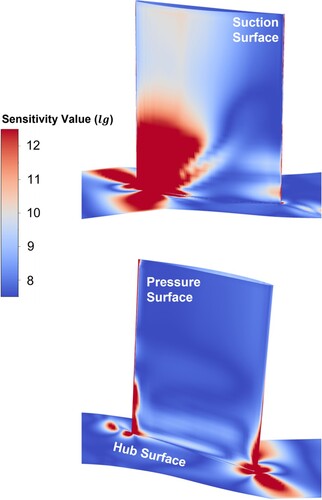
The sensitivity value of total pressure loss coefficient $\epsilon$ to the grid points on the cascade suction surface and hub surface are obtained at each design step, and the contours of sensitivity value for the prototype geometry are shown in Figure 12. The results show that the flow losses are quite sensitive to the geometrical morphing of the cascade leading edge on both the suction surface and the pressure surface near the end-wall region. In addition, the potential changes in the aerodynamic shape of the hub surface in conjunction with the cascade trailing edge near the end-wall region also significantly influence the overall compressor cascade performance. In this study, only the compressor cascade surface is optimised to reduce the total pressure losses, and the geometrical modifications on the end-wall (either hub or shroud surface) are not considered.

Figure 12. Contours of sensitivity value.

The adjoint optimisation stops after 30 design steps when the relative change in total pressure loss coefficient $\zeta$ between the latest design step and the previous design step becomes smaller than 1e-05. As a result, the total pressure loss coefficient $\zeta$ is finally reduced by 18.1% when compared to the baseline design. The static pressure rise coefficient $\psi$ is also increased by 8.1% when compared to the prototype. 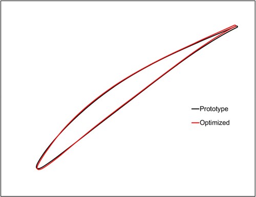Here the definition of static pressure rise coefficient $\psi$ is: (22) $\psi =(p_{s\mathrm{\_}outlet}-p_{s\mathrm{\_}inlet})/(p_{t\mathrm{\_}inlet}-p_{s\mathrm{\_}inlet})$(22) where $p_{s\mathrm{\_}outlet}$ is the static pressure in the outlet plane. Figure 13 shows the comparison of cascade near-hub airfoil profiles between the prototype and the optimised design. Compared to the prototype airfoil, the adjoint optimiser mainly attempts to modify the aerodynamic blade shape near the leading edge and trailing edge, which validates the conclusions derived from the sensitivity study shown in Figure 12. The compressor cascade airfoil near the hub region is rotated to align with the incoming flow and the curvature near the trailing edge is also modified to reduce the outflow deviation, which is similar to the ‘end-bend’ effect (Zheng and Li 2017). As a result, the incidence angles in the cascade lower-span region are reduced, and the flow separation losses are alleviated accordingly.

Figure 13. Comparison of cascade airfoil profiles near the hub region.

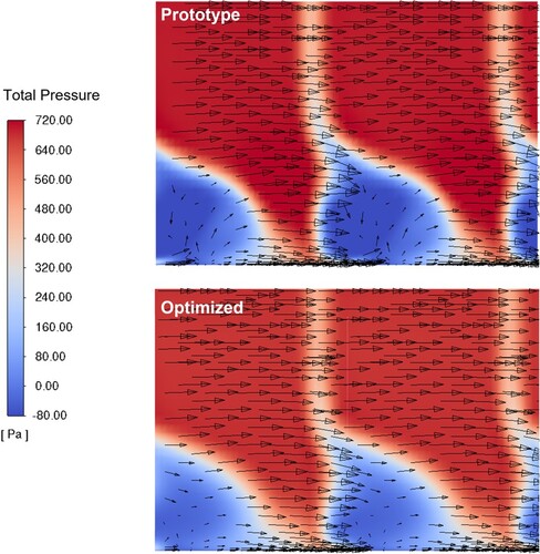
The WA model-based flow field comparison between the prototype and optimised compressor cascade passage is shown in Figure 14 to understand the flow mechanisms behind the performance improvement. In detail, the contours of the total pressure on the downstream plane surface (36.3% chord length downstream of cascade trailing edge) are plotted here in conjunction with the time-averaged 2D velocity vectors. Here the dark blue zone represents the region with high aerodynamic losses, which are mainly caused by the 3D corner separation flow. The 2D vector plots further show that this corner separation flow induces obvious secondary flow, and the shape modification characterised by the optimised cascade blade successfully reduces these secondary flow losses in terms of either the intensity or the size (the dark blue colour becomes light, and the size of high flow loss zone decreases in Figure 14). These qualitative changes in this contour plot finally contributes to the 18.1% reduction of total pressure loss within the cascade passage.

Figure 14. Flowfield comparison between prototype and optimised compressor cascade passage.

6. Conclusions

This paper has employed a recently developed one-equation Wray-Agarwal (WA) turbulence model to investigate the compressor cascade passage flow at different incidence angles. The WA turbulence model results are compared to experimental data in conjunction with the traditional Spalart-Allmaras (SA) model and k-ω Shear Stress Transport (SST) model. The cascade shape is then optimised by deploying the combination of the WA model flow field and the adjoint optimisation algorithm. The major conclusions can be drawn as follows:

1. Compared to the traditional SA model and k-ω SST model, the WA model gives the improved capability in predicting the total pressure loss downstream of the compressor cascade, although the prediction accuracy of turbulence models is reduced in simulating the significant flow separations near the end-wall region. On the mid-span section, the WA turbulence model results agree well with the experimental data.

2. Various turbulence length scales should be resolved in simulating the complex gas turbine flow field if the numerical prediction capability needs to be further improved. The WA model-based DES (Detached Eddy Simulation) results give the superior capability in predicting the compressor cascade aerodynamic losses characterised by large flow separation at the incidence angle of 4 degree compared to the other traditional turbulence models.

3. The combination of the WA model-based flow field and the adjoint optimisation algorithm successfully reduced the flow losses inside the cascade passage. The total pressure loss coefficient was reduced by 18.1%, and the static pressure rise capability increased by 8.1% compared to the prototype. The main flow mechanisms are that both the intensity and size of the end-wall corner separation are reduced due to the geometry modification of the cascade guided by the adjoint optimiser.

Acknowledgements

The first author would like to gratefully thank the support of the grant from the Marie Skłodowska-Curie Actions Individual Fellowship (MSCA-IF-MENTOR-101029472).

Disclosure statement

No potential conflict of interest was reported by the author(s).

Additional information

Funding

This work was supported by H2020 Marie Skłodowska-Curie Actions: [Grant Number MSCA-IF-MENTOR-101029472].

Appendix A

The governing Navier-Stokes equations are spatially discretized based on the finite volume formulation as given below: (A1) $V_i\frac{\mathrm{\partial }{Q}_i}{\mathrm{\partial }t}=-\sum _{cell\mathrm{\_}faces}F(Q_i).nS$(A1) where $V_i$ denotes the volume of the i-th cell, $Q_i$ denotes the vector of the conserved variables and $F$ denotes the flux vector. $Q_i$ and $F$ are given by the equations: (A2) $\begin{array}{rl}{Q}_i& =[\rho \rho u\rho v\rho w\rho E{]}^T\end{array}$(A2) (A3) $\begin{array}{rl}F& =[HJK{]}^T\end{array}$(A3) (A4) $\begin{array}{rl}H& =\left[\begin{array}{c}\rho u\\ \rho u^2+p-{\tau }_{xx}\\ \rho uv-{\tau }_{xy}\\ \rho uw-{\tau }_{xz}\\ u(\rho E+p)-u{\tau }_{xx}-v{\tau }_{xy}-w{\tau }_{xz}\end{array}\right]\end{array}$(A4) (A5) $\begin{array}{rl}J& =\left[\begin{array}{c}\rho v\\ \rho v^2+p-{\tau }_{yy}\\ \rho vu-{\tau }_{yx}\\ \rho vw-{\tau }_{yz}\\ v(\rho E+p)-u{\tau }_{yx}-v{\tau }_{yy}-w{\tau }_{yz}\end{array}\right]\end{array}$(A5) (A6) $\begin{array}{rl}K& =\left[\begin{array}{c}\rho w\\ \rho w^2+p-{\tau }_{zz}\\ \rho wu-{\tau }_{zx}\\ \rho wv-{\tau }_{zy}\\ w(\rho E+p)-u{\tau }_{zx}-v{\tau }_{zy}-w{\tau }_{zz}\end{array}\right]\end{array}$(A6) where $\rho$ denotes the fluid density and $u,v,w$ denote the flow velocity components in the Cartesian frame. For the convenience of derivation, we replace the right side of equation (A1) with $-\sum _{cel{l}_{faces}}F(Q_i).nS=-G_i(Q_i)$. Thus equation (A1) becomes: (A7) $V_i\frac{\mathrm{\partial }{Q}_i}{\mathrm{\partial }t}=-G_i(Q_i)$(A7)

Thus, the derivative of the objective function $I$ to the design variable α is given by: (A8) $\frac{dI}{d\alpha }=\left[{\left(\frac{\mathrm{\partial }I}{\mathrm{\partial }Q}\right)}^T+{\lambda }^T\frac{\mathrm{\partial }G}{\mathrm{\partial }Q}\right]\frac{dQ}{d\alpha }+\frac{\mathrm{\partial }I}{\mathrm{\partial }\alpha }+{\lambda }^T\frac{\mathrm{\partial }G}{\mathrm{\partial }\alpha }$(A8) and the adjoint equation is given by: (A9) ${\left(\frac{\mathrm{\partial }I}{\mathrm{\partial }Q}\right)}^T+{\lambda }^T\frac{\mathrm{\partial }G}{\mathrm{\partial }Q}=0$(A9) Here an implicit method is used for the temporal discretization of equation (A7): (A10) $\frac{Q^{n+1}-Q^n}{\mathrm{\Delta }t}=-G(Q^{n+1})$(A10) The introduction of first-order Taylor expansion in equation (A10) gives: (A11) $\left[\frac{1}{\mathrm{\Delta }t}+\frac{\mathrm{\partial }G(Q^n)}{Q^n}\right](Q^{n+1}-Q^n)=-G(Q^n)$(A11) Equation (A11) now becomes a linear system. More details in solving the linearised adjoint equation considering various boundary conditions can be found in Ref. [Moigne 2002].

References

- Bradshaw, P. 1996. “Turbulence Modeling with Application to Turbomachinery.” Progress in Aerospace Sciences 32 (6): 575–624. doi:10.1016/S0376-0421(96)00003-6
- Chen, J., and D. Whitfield. 1993. “Navier-Stokes Calculations for the Unsteady Flowfield of Turbomachinery.” American Institute of Aeronautics and Astronautics (AIAA) Paper, AIAA-93-0676.
- Chen, Q., and W. Xu. 1998. “A Zero-Equation Turbulence Model for Indoor Airflow Simulation.” Energy and Buildings 28 (2): 137–144. doi:10.1016/S0378-7788(98)00020-6
- Dawes, W. N. 1988. “Development of a 3d Navier Stokes solver for application to all types of turbomachinery,” American Society of Mechanical Engineers (ASME) Paper, 88-GT-70.
- Denton, J. D. 1975. “A Time Marching Method for Two- and Three- Dimensional Blade to Blade Flows,” Aeronautical Research Council Reports and Memoranda, Report No. ARC/R&M-3775.
- Everitt, J. N., and Z. S. Spakovszky. 2013. “An Investigation of Stall Inception in Centrifugal Compressor Vaned diffuser1.” Journal of Turbomachinery 135 (1): 011025. doi:10.1115/1.4006533
- Fares, E., and W. Schröder. 2005. “A General one-Equation Turbulence Model for Free Shear and Wall-Bounded Flows.” Flow, Turbulence and Combustion 73 (3): 187–215. doi:10.1007/s10494-005-8625-y
- Gao, F., W. Ma, G. Zambonini, J. Boudet, X. Ottavy, L. Lu, and L. Shao. 2015. “Large-eddy Simulation of 3-D Corner Separation in a Linear Compressor Cascade.” Physics of Fluids 27 (8): 085105. doi:10.1063/1.4928246
- Han, X., M. Rahman, and R. K. Agarwal. 2018. “Development and Application of Wall-distance-free Wray-Agarwal Turbulence Model (WA2018).” American Institute of Aeronautics and Astronautics (AIAA) Paper, AIAA 2018-0593.
- Han, X., T. Wray, and R. K. Agarwal. 2017. “Application of a New DES Model Based on Wray-Agarwal Turbulence Model for Simulation of Wall-bounded Flows with Separation.” American Institute of Aeronautics and Astronautics (AIAA) Paper, AIAA 2017-3966.
- Han, X., T. J. Wray, C. Fiola, and R. K. Agarwal. 2015. “Computation of Flow in S Ducts with Wray–Agarwal one-Equation Turbulence Model.” Journal of Propulsion and Power 31 (5): 1338–1349. doi:10.2514/1.B35672
- Hawthorne, W. R., and R. A. Novak. 1969. “The Aerodynamics of Turbo-Machinery.” Annual Review of Fluid Mechanics 1 (1): 341–366. doi:10.1146/annurev.fl.01.010169.002013
- Ji, L., W. Li, W. Shi, and R. K. Agarwal. 2021. “Application of Wray–Agarwal Turbulence Model in Flow Simulation of a Centrifugal Pump with Semispiral Suction Chamber.” Journal of Fluids Engineering 143 (3): 031203. doi:10.1115/1.4049050
- Li, Z. H., and X. Q. Zheng. 2017. “Review of Design Optimization Methods for Turbomachinery Aerodynamics.” Progress in Aerospace Sciences 93: 1–23. doi:10.1016/j.paerosci.2017.05.003
- Ma, W. 2012. “Experimental Investigation of Corner Stall in a Linear Compressor Cascade.” Doctoral dissertation, Ecole Centrale de Lyon.
- Ma, W., X. Ottavy, L. Lu, and L. Francis. 2013. “Intermittent Corner Separation in a Linear Compressor Cascade.” Experiments in Fluids 54 (6): 1–17. doi:10.1007/s00348-013-1546-y
- Menter, F. R. 1992. “Improved Two-Equation K-Omega Turbulence Models for Aerodynamic Flows.” NASA Technical Report No. 93:22809.
- Moigne, A. 2002. “A Discrete Navier-Stokes Adjoint Method for Aerodynamic Optimization of Blended Wing-Body Configurations.” Cranfield University, PhD thesis.
- Montomoli, F., H. P. Hodson, and L. Lapworth. 2011. “RANS–URANS in Axial Compressor, a Design Methodology.” Proceedings of the Institution of Mechanical Engineers, Part A: Journal of Power and Energy 225 (3): 363–374. doi:10.1177/2041296710394267
- Pope, S. B., and B. P. Stephen. 2000. Turbulent Flows. Cambridge, UK: Cambridge University Press.
- Schobeiri, M. T., and S. Abdelfattah. 2013. “On the Reliability of RANS and URANS Numerical Results for High-Pressure Turbine Simulations: A Benchmark Experimental and Numerical Study on Performance and Interstage Flow Behavior of High-Pressure Turbines at Design and off-Design Conditions Using two Different Turbine Designs.” Journal of Turbomachinery 135 (6): 061012. doi:10.1115/1.4024787
- Spalart, P., and A. Steven. 1992. “A One-equation Turbulence Model for Aerodynamic Flows.” American Institute of Aeronautics and Astronautics (AIAA) Paper, AIAA-92-0439.
- Wray, T. J. 2016. “Development of a One-equation Eddy Viscosity Turbulence Model for Application to Complex Turbulent Flows.” Doctoral dissertation, Washington University in St. Louis.
- Wray, T. J., and R. K. Agarwal. 2015. “Low-Reynolds-number one-Equation Turbulence Model Based on k-ω Closure.” AIAA Journal 53 (8): 2216–2227. doi:10.2514/1.J053632
- Yi, O., K. L. Tang, Y. Xiang, H. K. Zou, G. W. Chu, R. K. Agarwal, and J. F. Chen. 2019. “Evaluation of Various Turbulence Models for Numerical Simulation of a Multiphase System in a Rotating Packed bed.” Computers & Fluids 194: 104296. doi:10.1016/j.compfluid.2019.104296
- Zheng, X. Q., and Z. H. Li. 2017. “Blade-end Treatment to Improve the Performance of Axial Compressors: An Overview.” Progress in Aerospace Sciences 88: 1–14. doi:10.1016/j.paerosci.2016.09.001