Zig-Zag Sampling for Discrete Structures and Nonreversible Phylogenetic MCMC

Abstract

We construct a zig-zag process targeting a posterior distribution defined on a hybrid state space consisting of both discrete and continuous variables. The construction does not require any assumptions on the structure among discrete variables. We demonstrate our method on two examples in genetics based on the Kingman coalescent, showing that the zig-zag process can lead to efficiency gains of up to several orders of magnitude over classical Metropolis–Hastings algorithms, and that it is well suited to parallel computation. Our construction resembles existing techniques for Hamiltonian Monte Carlo on a hybrid state space, which suffers from implementationally and analytically complex boundary crossings when applied to the coalescent. We demonstrate that the continuous-time zig-zag process avoids these complications. Supplementary materials for this article are available online.

Keywords:

• Bayesian inference
• Coalescent
• Hybrid state space
• Piecewise deterministic Markov process
• Zig-zag process

1 Introduction

The zig-zag process is a nonreversible, piecewise deterministic Markov process introduced by Bierkens and Roberts (2017); Bierkens, Fearnhead, and Roberts (2019b) for continuous-time MCMC. It has several advantages over reversible methods such as Metropolis–Hastings (Hastings 1970) and Gibbs sampling (Gelfand and Smith 1990): it avoids diffusive backtracking which slows their mixing, and is rejection-free so that no computation is wasted on rejected moves.

In brief, the generator of the zig-zag process ${({\mathbf{x}}_t,{\mathbf{v}}_t)}_{t\ge 0}$ targeting the probability density (with respect to the product of the Lebesgue and counting measures) $\tilde{\pi }(\mathbf{x},\mathbf{v}):=\pi (\mathbf{x})/2^d$ on a state space $X\times {\{-1,1\}}^d\subseteq {\mathbb{R}}^d\times {\{-1,1\}}^d$ is$$Lf(\mathbf{x},\mathbf{v})=\sum _{i=1}^d{v}_i{\partial }_{i}f(\mathbf{x},\mathbf{v})+\sum _{i=1}^d{\lambda }_i(\mathbf{x},\mathbf{v})(f(\mathbf{x},F_i\mathbf{v})-f(\mathbf{x},\mathbf{v})),$$where ${\partial }_i$ is the derivative with respect to x_i , and F_i flips the sign of v_i . The flip rates(1) $${\lambda }_i(\mathbf{x},\mathbf{v}):={(-v_i{\partial }_i\hspace{0.17em}\text{log}\hspace{0.17em}(\tilde{\pi }(\mathbf{x},\mathbf{v})))}^{+}$$(1) with ${(x)}^{+}:=\max \{x,0\}$, ensure that ${({\mathbf{x}}_t,{\mathbf{v}}_t)}_{t\ge 0}$ leaves $\tilde{\pi }(\mathbf{x},\mathbf{v})$ invariant (Bierkens, Fearnhead, and Roberts 2019b, theorem 2.2). In words, the coordinates of ${\mathbf{x}}_t$ move at constant velocities ${\mathbf{v}}_t$ until a flip at coordinate i, when the corresponding velocity changes sign.

To date, the zig-zag processes have been applied to targets such as the Curie–Weiss model (Bierkens and Roberts 2017) and logistic regression (Bierkens, Fearnhead, and Roberts 2019b), whose state spaces have simple geometric structures with natural notions of direction and velocity. Discrete variables (other than the velocities) have been restricted to cases with simple partial orders, such as model selection (Chevalier, Fearnhead, and Sutton 2020; Gagnon and Doucet 2021). We construct a zig-zag process on a general hybrid state space with both continuous and discrete coordinates, without imposing any structure on discrete coordinates. This is done by introducing a separate space of continuous variables for each value of the discrete variable, introducing boundaries into the continuous spaces, and updating the discrete variable when boundaries are hit. The strategy takes advantage of the full generality of piecewise-deterministic Markov processes (Davis 1993, sec. 24), and is resembles similar work for Hamiltonian Monte Carlo (HMC) (Dinh et al. 2017; Nishimura, Dunson, and Lu 2020). Our method can also been seen of as a generalization of the zig-zag process on a restricted domain (Bierkens et al. 2018) to a union of many restricted sub-domains, with jumps between sub-domains at boundary hitting events. We illustrate our method with an application to the coalescent (Kingman 1982): a tree-valued target with continuous branch lengths, discrete tree topologies with no natural partial order, and no canonical geometric structure.

The coalescent examples illustrate the need for methods which are implementable on complex state spaces. They are also of interest because existing MCMC algorithms for coalescents tend to mix slowly. The key difficulty lies in designing Metropolis–Hastings proposal distributions which combine efficient exploration with a high acceptance rate (Mossel and Vigoda 2005; Höhna, Defoin-Platel, and Drummond 2008; Lakner et al. 2008). Workarounds consist of empirical searches for efficient proposals (Höhna and Drummond 2012; Aberer, Stamatakis, and Ronquist 2016) or Metropolis-coupled MCMC (Geyer 1992). The former does not scale to problems for which empirical optimization is infeasible. The latter helps mixing between modes, but does not overcome low acceptance rates or the backtracking behavior of reversible MCMC.

The zig-zag process has some similarities with HMC (Neal 2010), which augments the state space with momentum and uses Hamiltonian dynamics to propose large steps which are accepted with high probability, though they are not rejection-free. Like the zig-zag process, HMC requires gradient information and a suitable geometric embedding of the target. Dinh et al. (2017) provided those for the coalescent using an orthant complex construction of phylogenetic tree space (Billera, Holmes, and Vogtmann 2001). Our examples differ from the method of Dinh et al. (2017) in three ways. First, we replace the embedding of Billera, Holmes, and Vogtmann (2001) with τ-space (Gavryushkin and Drummond 2016), which is better suited to ultrametric trees. Second, the zig-zag process is readily implementable on τ-space via Poisson thinning without a numerical integrator such as leap-prog (Dinh et al. 2017, algorithm 1). Finally, the zig-zag process has simple boundary behavior between orthants and does not require boundary smoothing (Dinh et al. 2017, sec. 3.3), chiefly because discontinuous gradients are easier to handle on continuous rather than discretized paths.

The rest of the paper is structured as follows. Section 2 defines the zig-zag algorithm with discrete and continuous variables, and proves that it has the desired invariant distribution. Section 3 recalls the coalescent and the τ-space embedding. In Sections 4 and 5 we recall the popular infinite and finite sites models of mutation, derive zig-zag processes for each, and demonstrate their performance via simulation studies. Section 6 concludes with a discussion. The algorithms and datasets used in the simulation studies are available at https://github.com/JereKoskela/tree-zig-zag.

2 Zig-zag on Hybrid Spaces

The definition of our zig-zag process follows (Davis 1993, sec. 24). Let $\mathbb{F}$ be a countable set. For each $m\in \mathbb{F}$, let ${\Omega }_m^o$ be an open subset of ${\mathbb{R}}^d,\overline{{\Omega }_m^o}$ be its closure, and $\partial {\Omega }_m^{*}:=\overline{{\Omega }_m^o}\setminus {\Omega }_m^o$ be its boundary. We assume that ${\{\partial {\Omega }_m^{*}\}}_{m\in \mathbb{F}}$ are piecewise Lipschitz and denote by $\partial {\Omega }_m$ the restriction of $\partial {\Omega }_m^{*}$ to noncorner points. Let ${\Omega }^o:={\cup }_{m\in \mathbb{F}}{\Omega }_m^o=\{(m,\mathbf{x}):m\in \mathbb{F},\mathbf{x}\in {\Omega }_m^o\}$ and $\partial \Omega :={\cup }_{m\in \mathbb{F}}\partial {\Omega }_m$. For a point $(m,\mathbf{x})\in \partial {\Omega }_m$, let $n(m,\mathbf{x})$ be the outward unit normal, and let ${\Gamma }^{\pm }(m,\mathbf{x}):=\{\mathbf{v}\in {\{-1,1\}}^d:\pm (\mathbf{v}·n(m,\mathbf{x}))>0\}$ be the sets of velocities with which a zig-zag process can exit (+) or enter (–) ${\Omega }_m^o$ at $\mathbf{x}$. Zig-zag dynamics imply $\mathbf{v}\in {\Gamma }^{+}(m,\mathbf{x})\iff -\mathbf{v}\in {\Gamma }^{-}(m,\mathbf{x})$. We also define ${\Gamma }^{\pm }(\partial \Omega ):={\cup }_{(m,\mathbf{x})\in \partial \Omega }(\{(m,\mathbf{x})\}\times {\Gamma }^{\pm }(m,\mathbf{x}))$ and ${\Omega }^{*}:=({\Omega }^o\times {\{-1,1\}}^d)\cup {\Gamma }^{-}(\partial \Omega )$. Integrals over ${\Omega }^o$ and $\partial \Omega$, or subsets thereof, are taken to incorporate discrete sums in the $m\in \mathbb{F}$ coordinate.

The zig-zag process ${(m_t,{\mathbf{x}}_t,{\mathbf{v}}_t)}_{t\ge 0}$ is defined on ${\Omega }^{*}$, with target $\tilde{\pi }(m,\mathbf{x},\mathbf{v}):=\pi (m,\mathbf{x})/2^d$ on ${\Omega }^{*}\cup {\Gamma }^{+}(\partial \Omega )$ for a given density $\pi (m,\mathbf{x})$. At $(m,\mathbf{x},\mathbf{v})\in {\Omega }^{*}$, the process moves with velocity $\mathbf{v}$ and each coordinate v_i flips at rate $\lambda (m,\mathbf{x},\mathbf{v})$, defined as in (1) since m is fixed between boundary hitting events. When $(m,\mathbf{x},\mathbf{v})\in {\Gamma }^{+}(\partial \Omega )$, the process jumps according to a Markov kernel $Q:{\Gamma }^{+}(\partial \Omega )\mapsto \mathcal{P}({\Gamma }^{-}(\partial \Omega ))$, where $\mathcal{P}(A)$ denotes the set of probability measures on $(A,\mathcal{B}(A))$. We assume that Q and $\tilde{\pi }$ satisfy the skew-detailed balance condition(2) $$\begin{array}{c}\tilde{\pi }(m,\mathbf{x},\mathbf{v})Q(m,\mathbf{x},\mathbf{v};j,\mathrm{d}\mathbf{y},\mathbf{w})\mathrm{d}\mathbf{x}\\ \hspace{1em}=\tilde{\pi }(j,\mathbf{y},-\mathbf{w})Q(j,\mathbf{y},-\mathbf{w};m,\mathrm{d}\mathbf{x},-\mathbf{v})\mathrm{d}\mathbf{y}\end{array}$$(2) for any $(m,\mathbf{x},\mathbf{v})\in {\Gamma }^{+}(\partial \Omega )$ and $(j,\mathbf{y},\mathbf{w})\in {\Gamma }^{-}(\partial \Omega )$, as well as(3) $${\int }_{(j,\mathbf{y})\in \partial \Omega }\sum _{\mathbf{w}\in {\Gamma }^{-}(j,\mathbf{y})}(\mathbf{w}·n(j,\mathbf{y}))Q(m,\mathbf{x},\mathbf{v};j,\mathrm{d}\mathbf{y},\mathbf{w})=-\mathbf{v}·n(m,\mathbf{x}),$$(3) for any $(\mathbf{x},\mathbf{v})\in {\Gamma }^{+}(\partial \Omega )$, and exclude jumps to paths pointing into corners by assuming(4) $$\begin{array}{c}{\int }_{(m,\mathbf{x})\in \partial \Omega }{\sum }_{\mathbf{v}\in {\Gamma }^{+}(m,\mathbf{x})}{\int }_{(j,\mathbf{y})\in \partial \Omega }{\sum }_{\mathbf{w}\in {\Gamma }^{-}(j,\mathbf{y})}\\ \mathrm{\hspace{1em}}\mathrm{\hspace{1em}}{1}_{({\cup }_{m\in \mathbb{F}}\partial {\Omega }^{*})\setminus \partial \Omega }(j,\mathbf{y}+T_{{\Gamma }^{+}(\partial \Omega )}(j,\mathbf{y},\mathbf{w})\mathbf{w})\\ \mathrm{\hspace{1em}}\mathrm{\hspace{1em}}\times Q(m,\mathbf{x},\mathbf{v};j,\mathrm{d}\mathbf{y},\mathbf{w})\mathrm{d}\mathbf{x}=0,\end{array}$$(4) where $T_{{\Gamma }^{+}(\partial \Omega )}(j,\mathbf{y},\mathbf{w})$ is the time the line ${(j,\mathbf{y}+t\mathbf{w})}_{t\ge 0}$ hits ${\Gamma }^{+}(\partial \Omega )$. We will abuse notation and use $\tilde{\pi }(m,\mathbf{x},\mathbf{v})\mathrm{d}\mathbf{x}$ as the target density and Lebesgue measure on ${\Omega }^o$, and as their restrictions to the surface $\partial \Omega$, on which $\tilde{\pi }$ is not a probability density.

By Davis (1993, theorem 26.14), the zig-zag process with dynamics defined above is a piecewise-deterministic Markov process with extended generator(5) $$\begin{array}{c}Lf(m,\mathbf{x},\mathbf{v})=\sum _{i=1}^d{v}_i{\partial }_{i}f(m,\mathbf{x},\mathbf{v})\\ \hspace{1em}+\sum _{i=1}^d{\lambda }_i(m,\mathbf{x},\mathbf{v})(f(m,\mathbf{x},F_i\mathbf{v})-f(m,\mathbf{x},\mathbf{v})),\end{array}$$(5) whose domain D(L) consists of measurable functions $f(m,\mathbf{x},\mathbf{v})$ on ${\Omega }^{*}$ satisfying:

1. For each $(m,\mathbf{x},\mathbf{v})\in {\Gamma }^{+}(\partial \Omega )$, the limit $\underset{t\to 0}{\lim }f(m,\mathbf{x}-t\mathbf{v},\mathbf{v})=:f(m,\mathbf{x},\mathbf{v})$ exists.

2. For each $(m,\mathbf{x},\mathbf{v})\in {\Omega }^{*}$, the function $t\mapsto f(m,\mathbf{x}+t\mathbf{v},\mathbf{v})$ is absolutely continuous on $t\in [0,T_{{\Gamma }^{+}(\partial \Omega )}(m,\mathbf{x},\mathbf{v}))$.

3. For $(m,\mathbf{x},\mathbf{v})\in {\Gamma }^{+}(\partial \Omega )$,(6) $$f(m,\mathbf{x},\mathbf{v})={\int }_{(j,\mathbf{y})\in \partial \Omega }\sum _{\mathbf{w}\in {\Gamma }^{-}(\mathbf{y})}f(j,\mathbf{y},\mathbf{w})Q(m,\mathbf{x},\mathbf{v};j,\mathrm{d}\mathbf{y},\mathbf{w}).$$(6)

4. The random variable ${\sum }_{k=1}^{n}f(m_{T_k},{\mathbf{x}}_{T_k},{\mathbf{v}}_{T_k})-f(m_{T_k},{\mathbf{x}}_{T_k-},{\mathbf{v}}_{T_k-})$ is integrable for each $n\in \mathbb{N}$, where ${\left\{T_k\right\}}_{k\ge 1}$ are the successive jump times (both velocity flips and jumps due to hitting a boundary) of ${(m_t,{\mathbf{x}}_t,{\mathbf{v}}_t)}_{t\ge 0}$.

For a set A, let B(A) and $C^1(A)$ be the respective spaces of bounded and continuously differentiable functions on A. Let $C_b^1(A):=B(A)\cap C^1(A)$. For t > 0, we define$$N_t:=\#\left\{\text{velocity}\mathrm{ }\text{flips}\mathrm{ }\text{and}\mathrm{ }\text{boundary}\mathrm{ }\text{jumps}\mathrm{ }\text{in}\mathrm{ }{(m_s,{\mathbf{x}}_s,{\mathbf{v}}_s)}_{s=0}^t\right\}.$$

Theorem 1.

Suppose $\mathbb{F}$ is finite, $\tilde{\pi }(m,·,\mathbf{v})\in C^1({\Omega }_m^o)$ for each $\mathbf{v}\in {\{-1,1\}}^d$ and $m\in \mathbb{F},\tilde{\pi }>0$ on ${\Omega }^o\times {\{-1,1\}}^d$, that $Q(m,\mathbf{x},\mathbf{v};·)$ has compact support for each $(m,\mathbf{x},\mathbf{v})\in {\Gamma }^{+}(\partial \Omega )$, and for each t > 0 and $(m,\mathbf{x},\mathbf{v})\in {\Omega }^{*}$,(7) $$\mathbb{E}\left[N_t\right|(m_0,{\mathbf{x}}_0,{\mathbf{v}}_0)=(m,\mathbf{x},\mathbf{v})]<\infty .$$(7)

Suppose the initial distribution of $(m,\mathbf{x})$ has a density on ${\Omega }^{*}$ and that (2)–(4) hold. Then the zig-zag process with generator (5) and domain D(L) as described above has stationary distribution $\tilde{\pi }$.

Proof.

Provided in the supplementary materials. □

Remark 1.

In addition to having the right invariant distribution, a practical algorithm needs to be ergodic. To discuss ergodicity of the zig-zag process ${(m_t,{\mathbf{x}}_t,{\mathbf{v}}_t)}_{t\ge 0}$ from Theorem 1, let ${\left\{{(m_t^j,{\mathbf{x}}_t^j,{\mathbf{v}}_t^j)}_{t\ge 0}\right\}}_{j\in \mathbb{F}}$ be zig-zag processes restricted to respective spaces ${\Omega }_j^o$ by boundary jump kernels $Q^j:{\cup }_{\mathbf{x}\in \partial {\Omega }_j}[(j,\mathbf{x})\times {\Gamma }^{+}(j,\mathbf{x})]\mapsto \mathcal{P}({\cup }_{\mathbf{x}\in \partial {\Omega }_j}[(j,\mathbf{x})\times {\Gamma }^{-}(j,\mathbf{x})])$, each with target proportional to $\tilde{\pi }(j,·,·)$. When $\mathbb{F}$ is finite, a sufficient condition for ergodicity of the global process ${(m_t,{\mathbf{x}}_t,{\mathbf{v}}_t)}_{t\ge 0}$ is that ${\left\{{(m_t^j,{\mathbf{x}}_t^j,{\mathbf{v}}_t^j)}_{t\ge 0}\right\}}_{j\in \mathbb{F}}$ are all ergodic, and that(8) $$\begin{array}{c}{\int }_{\mathbf{x}\in \partial {\Omega }_m}\sum _{\mathbf{v}\in {\Gamma }^{+}(m,\mathbf{x})}{\int }_{\mathbf{y}\in \partial {\Omega }_j}\sum _{\mathbf{w}\in {\Gamma }^{-}(j,\mathbf{y})}Q(m,\mathbf{x},\mathbf{v};j,\mathrm{d}\mathbf{y},\mathbf{w})\\ \tilde{\pi }(m,\mathbf{x},\mathbf{v})\mathrm{d}\mathbf{x}>0,\end{array}$$(8) for ordered pairs $(m,j)\in {\mathbb{F}}^2$ which form a cycle spanning the support of $\tilde{\pi }$. Bierkens, Roberts, and Zitt (2019) provide conditions for ergodicity of single-domain zig-zag processes.

We conclude this section with a pseudocode specification of our zig-zag algorithm.

Algorithm 1 Simulation the zig-zag process targeting $\tilde{\pi }$

Require: Initial condition $(m,{\mathbf{x}}_0,{\mathbf{v}}_0)$, target $\tilde{\pi }$, jump kernel Q, terminal time $t_{\text{end}}$

1. Set $t\leftarrow 0,m_0\leftarrow m,\mathbf{x}\leftarrow {\mathbf{x}}_0,\mathbf{v}\leftarrow {\mathbf{v}}_0$

2. while $t<t_{\text{end}}$ do

3. Set $\tau \leftarrow T_{{\Gamma }^{+}(\partial \Omega )}(m,\mathbf{x},\mathbf{v})$ and $I\leftarrow 0$. ⊳ $I=0\Rightarrow$ boundary hit.

4. for $i\in \{1,2,\dots ,d-1,d\}$ do

5. Sample $U\sim \hspace{0.17em}\text{Exp}\hspace{0.17em}(1)$.

6. Set ρ to be the solution of ${\int }_0^{\rho }{\lambda }_i(m,\mathbf{x}+s\mathbf{v},\mathbf{v})\mathrm{d}s=U$.

7. if $\rho <\tau$ then

8. Set $\tau \leftarrow \rho$ and $I\leftarrow i$

9. Set $t\leftarrow t+\tau ,\mathbf{x}\leftarrow \mathbf{x}+\tau \mathbf{v}$

10. if I > 0 then

11. Set $v_I\leftarrow -v_I$

12. else

13. Set $(m,\mathbf{x},\mathbf{v})\leftarrow (j,\mathbf{y},\mathbf{w})\sim Q(m,\mathbf{x},\mathbf{v};·,·,·)$

3 The Coalescent and a Geometric Embedding

An ultrametric binary tree with n labeled leaves is a rooted binary tree in which each leaf is an equal graph distance away from the root. We follow Gavryushkin and Drummond (2016) and encode such a tree with leaf labels $\{1,\dots ,n\}$ as the pair $(E_n,{\mathbf{t}}_n)$, where E_n is a ranked topology and ${\mathbf{t}}_n\in {(0,\infty )}^{n-1}$. The continuous variables ${\mathbf{t}}_n$ encode times between mergers. The time from the leaves to the first merger is t₁, and subsequent t_i variables are times between successive mergers. 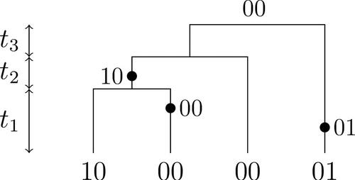The ranked topology E_n is an $(n-1)$-tuple of pairs of labels, where the ith pair specifies the two child nodes of the ith merger. Nonleaf nodes are labeled by the leaves they subtend. For example, the ranked topology$$E_4=(E_{4,1},E_{4,2},E_{4,3}):=(\{1,2\},\{\{1,2\},3\},\{\{1,2,3\},4\})$$encodes the four leaf caterpillar tree depicted in Figures 3 and 7 with nodes labeled left to right. We order the two entries of $E_{n,i}$ by their least element for definiteness.

The coalescent (Kingman 1982) is a seminal model for the genetic ancestry of samples from large populations. Under the coalescent, a tree $(E_n,{\mathbf{t}}_n)$ has probability density(9) $$\pi (E_n,{\mathbf{t}}_n)\mathrm{d}{\mathbf{t}}_n:=\hspace{0.17em}\text{exp}\hspace{0.17em}(-\sum _{i=1}^{n-1}\left(\begin{array}{c}n+1-i\\ 2\end{array}\right)t_i)\mathrm{d}{\mathbf{t}}_n,$$(9) which arises as the law of a tree constructed by starting a lineage from each leaf, and merging each pair of lineages at rate 1 until the most recent common ancestor (MRCA) is reached. The success of the coalescent is due to robustness: distributions of ancestries of a large class of individual-based models converge to the coalescent in the infinite population limit under suitable rescalings of time. For details, see, for example, Wakeley (2009).

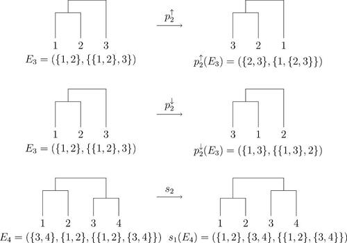
We define swap operators s_i for $i\in \{2,\dots ,n-2\}:E_{n,i-1}\notin E_{n,i}$ via$$\begin{array}{c}{s}_i(E_n):=(E_{n,1}^{\prime },\dots ,E_{n,n-1}^{\prime })\mathrm{ }\text{where}\\ \mathrm{ }{E}_{n,k}^{\prime }:=\{\begin{array}{cc}{E}_{n,k}\hfill & \mathrm{ }\text{for}\mathrm{ }k<i-1\mathrm{ }\text{or}\mathrm{ }k>i,\hfill \\ E_{n,i}\hfill & \mathrm{ }\text{for}\mathrm{ }k=i-1,\hfill \\ E_{n,i-1}\hfill & \mathrm{ }\text{for}\mathrm{ }k=i.\hfill \end{array}\end{array}$$

In words, s_i swaps the order of the $(i-1)$th and ith mergers. We also define pivot operators $p_i^{\downarrow }$ and $p_i^{\uparrow }$ for $i\in \{2,\dots ,n-1\}:E_{n,i-1}\in E_{n,i}$ as(10) $$\begin{array}{c}{p}_i^{\downarrow }(E_n):=(E_{n,1}^{\prime },\dots ,E_{n,n-1}^{\prime })\mathrm{ }\text{with}\\ E_{n,k}^{\prime }:=\{\begin{array}{cc}{E}_{n,k}\hfill & \mathrm{ }\text{for}\mathrm{ }k\notin \{i-1,i\},\hfill \\ \{E_{n,i-1}^{\downarrow },E_{n,i}^s\}\hfill & \mathrm{ }\text{for}\mathrm{ }k=i-1,\hfill \\ \{E_{n,i-1}^{\prime },E_{n,i-1}^{\uparrow }\}\hfill & \mathrm{ }\text{for}\mathrm{ }k=i,\hfill \end{array}\end{array}$$(10) where $E_{n,i}^{\uparrow }$ (resp. $E_{n,i}^{\downarrow }$) is the entry of $E_{n,i}$ with the higher (resp. lower) least element, and $E_{n,i}^s$ is the sibling: the entry of $E_{n,i}$ that is not $E_{n,i-1}$. Pivot $p_i^{\uparrow }$ is defined by interchanging ↓ and ↑ in (10). The pivots are the two nearest neighbor interchanges between the ith merger and the merger involving its nearest child. Figure 1 illustrates all three operators.

Fig. 1 Operators $p_2^{\uparrow },p_2^{\downarrow }$, and s₂. The horizontal arrangement of leaves is arbitrary throughout this article; only vertical distance is meaningful.

Next we describe τ-space, which gives a geometric structure to the set of pairs $(E_n,{\mathbf{t}}_n)$. For fixed E_n , the space of ${\mathbf{t}}_n$-vectors is the orthant ${[0,\infty )}^{n-1}$. Each boundary point with t_i = 0 corresponds to a degenerate tree in which one of three things happens:

1. The two leaves of $E_{n,1}$ merge at time 0 if i = 1.

2. There are two simultaneous mergers if $E_{n,i-1}\notin E_{n,i}$.

3. There is a simultaneous merger of three lineages if $E_{n,i-1}\in E_{n,i}$.

Type 1 boundaries are boundaries of the whole τ-space. Type 2 boundaries separate orthants corresponding to two ranked topologies separated by an s_i -step. Trajectories crossing the boundary move from one ranked topology to the other. Type 3 boundaries separate the three orthants which resolve the triple merger into two binary mergers, which differ by a $p_i^{\downarrow }$ or $p_i^{\uparrow }$-step. A trajectory that crosses the boundary visits a tree with the triple merger. Figure 2 depicts the τ-space with three leaves, and a type 2 boundary in a general τ-space. An example with five leaves is depicted in (Gavryushkin and Drummond 2016, figure 2), and the ${\mathbf{t}}_n$ variables are illustrated in Figures 3 and 7 in Sections 4 and 5.

Fig. 2 (Left) τ-space with n = 3 embedded into ${\mathbb{R}}^3$. Each square is a copy of ${[0,\infty )}^2$ associated with the given topology. The coordinates $(t_1,t_2)$ are the respective time of the first merger, and the time between the first and second merger. The dot is the origin, and the line on which all three orthants intersect is a type 3 boundary consisting of trees in which all three leaves merge simultaneously at time t₁. The dashed lines are boundaries at $\infty$. (Right) A segment of τ-space depicting a type 2 boundary, in which each square represents ${[0,\infty )}^{n-1}$. Only the two orthants adjacent to the boundary are shown.

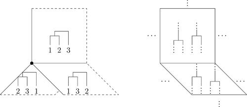
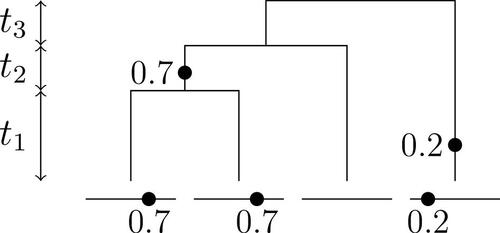
Fig. 3 A realization of the infinite sites model with n = 4, two mutations, three types, and $D_n=(\{0.7\},\{0.7\},\{\},\{0.2\})$. The holding times ${\mathbf{t}}_3$ are shown on the left.

We will use τ-space to construct zig-zag processes whose state spaces consist of tree topologies, branch lengths, and a scalar parameter introduced in the next section. The discrete variables $\mathbb{F}$ will be the ranked topologies, with the boundary crossings described above defining the boundary jump kernel Q. For more on τ-space, for example, existence and uniqueness of geodesics and Fréchet means, we refer to Gavryushkin and Drummond (2016).

4 The Infinite Sites Model

The infinite sites model (Watterson 1975) connects the coalescent tree to DNA sequence data by associating the MRCA with the unit interval (0, 1). Mutations with independent, $U(0,1)$-distributed locations accrue along branches of the tree (with branch lengths as specified by ${\mathbf{t}}_n$) at rate $\theta /2$. The type of a leaf consist of the mutations along branches separating it from the MRCA. We denote the resulting list of types of the leaves by D_n . A realization of a coalescent tree and associated D_n is shown in Figure 3. The typical task is to sample from the conditional law $(E_n,{\mathbf{t}}_n,\theta )|D_n$ corresponding to observing D_n , but not the tree which gave rise to it.

To handle mutations, we define F_n as the rooted graphical tree with $2n-1$ nodes, the first n of which are leaves labeled $1,\dots ,n$, while the remaining $n-1$ are labeled as in E_n . Edges connect children to their parents, and edge lengths are determined by ${\mathbf{t}}_n$. For an edge $\gamma \in F_n$, we denote by $c_{\gamma }$ and $p_{\gamma }$ the respective labels of the child and parent nodes of γ, by $m_{\gamma }$ the number of mutations on γ, and by $l_{\gamma }:=\sum _{t_j\in \gamma }{t}_j$ the edge length, where we write $t_i\in \gamma$ if t_i contributes to the length of γ in which case we say γ spans t_i .

Given a prior density ${\pi }_0(\theta )$ for θ, the posterior distribution of $(E_n,{\mathbf{t}}_n,\theta )|D_n$ follows from (9), the fact that the number of mutations on branch $\gamma \in F_n$ is Poisson($\theta l_{\gamma }/2$)-distributed given $l_{\gamma }$, and that mutations on distinct branches are independent. In particular,(11) $$\begin{array}{c}\pi (E_n,{\mathbf{t}}_n,\theta |D_n)\propto {\{\prod _{\gamma \in F_n}(\frac{\theta l_{\gamma }}{2})}^{m_{\gamma }}\}\\ \hspace{1em}\hspace{0.17em}\text{exp}\hspace{0.17em}(-\sum _{i=1}^{n-1}\frac{(n+1-i)(n+\theta -i)}{2}{t}_i){\pi }_0(\theta )\end{array}$$(11) provided E_n is consistent D_n , and π = 0 otherwise. This distribution can be sampled using a zig-zag algorithm by taking $\mathbb{F}$ to be the set of ranked topologies on n leaves which are consistent with D_n , as well as ${\Omega }_{E_n}^o:=\{({\mathbf{t}}_n,\theta )\in {(0,\infty )}^n\}$ and $\partial {\Omega }_{E_n}:=\{({\mathbf{t}}_n,\theta )\in {[0,\infty )}^n:t_i=0\mathrm{ }\text{for}\mathrm{ }\text{one}\mathrm{ }i\in \{1,\dots ,n-1\}\mathrm{ }\text{or}\mathrm{ }\theta =0\}$ for each $E_n\in \mathbb{F}$. In the boundary classification of Section 3, θ = 0 is another type 1 boundary. For $({\mathbf{t}}_n,\theta )\in \partial \Omega$, we define $k({\mathbf{t}}_n,\theta )$ as the index of the zero variable, taken to be n in the case of θ.

We augment the state space with n zig-zag velocities ${\mathbf{v}}_n$, of which $(v_1,\dots ,v_{n-1})$ drive ${\mathbf{t}}_n$ and v_n drives θ. For $\gamma \in F_n$, we also define $v_{\gamma }:=\sum _{j:t_j\in \gamma }{v}_j$ as the rate of change of $l_{\gamma }$. The boundary kernel Q is defined separately on each boundary type:(12) $$\begin{array}{c}Q(E_n,({\mathbf{t}}_n,\theta ),{\mathbf{v}}_n;·,·,·)\\ :=\{\text{}\begin{array}{cc}{\delta }_{\left\{E_n\right\}}(·)\otimes {\delta }_{\{({\mathbf{t}}_n,\theta )\}}(·)\otimes {\delta }_{\{F_{k({\mathbf{t}}_n,\theta )}({\mathbf{v}}_n)\}}(·)\hfill & \text{for}\mathrm{ }\text{type}\mathrm{ }1,\hfill \\ {\delta }_{\{s_{k({\mathbf{t}}_n,\theta )}(E_n)\}}(·)\otimes {\delta }_{\{({\mathbf{t}}_n,\theta )\}}(·)\otimes {\delta }_{\{F_{k({\mathbf{t}}_n,\theta )}({\mathbf{v}}_n)\}}(·)\hfill & \text{for}\mathrm{ }\text{type}\mathrm{ }2,\hfill \\ (\frac{{\delta }_{\{p_{k({\mathbf{t}}_n,\theta )}^{\uparrow }(E_n)\}}(·)}{2}+\frac{{\delta }_{\{p_{k({\mathbf{t}}_n,\theta )}^{\downarrow }(E_n)\}}(·)}{2})\otimes {\delta }_{\{({\mathbf{t}}_n,\theta )\}}(·)\hfill & \hfill \\ \hspace{1em}\otimes {\delta }_{\{F_{k({\mathbf{t}}_n,\theta )}({\mathbf{v}}_n)\}}(·)\hfill & \text{for}\mathrm{ }\text{type}\mathrm{ }3.\hfill \end{array}\end{array}$$(12)

At a type 1 boundary the process reflects back into ${\Omega }_{E_n}^o$ via a velocity flip. At a type 2 boundary it undergoes an s_i -step and a velocity flip to pass through the boundary. For type 3 boundaries it chooses an adjacent orthant uniformly at random.

In the interiors of orthants, velocity flip rates are(13) $$\begin{array}{c}{\lambda }_i(E_n,{\mathbf{t}}_n,\theta ;{\mathbf{v}}_n)\\ \hspace{1em}:={[v_i(\frac{(n+1-i)(n+\theta -i)}{2}-\sum _{\gamma \in F_n:t_i\in \gamma }\frac{m_{\gamma }}{l_{\gamma }})]}^{+},\end{array}$$(13) (14) $$\begin{array}{c}{\lambda }_{\theta }(E_n,{\mathbf{t}}_n,\theta ;{\mathbf{v}}_n)\\ \hspace{1em}:={[v_n(\sum _{i=1}^{n-1}\frac{n+1-i}{2}{t}_i-\frac{1}{\theta }\sum _{\gamma \in F_n}{m}_{\gamma }-{\partial }_{\theta }\hspace{0.17em}\text{log}\hspace{0.17em}({\pi }_0(\theta )))]}^{+}.\end{array}$$(14)

Simulating holding times with these rates is difficult due to the time intervals during which they vanish. One strategy is Poisson thinning via dominating rates consisting of only those terms in the round brackets in (13) and (14) whose sign matches that of the corresponding velocity v_i , but these can result in loose bounds and inefficient algorithms. Instead, we define $t_n:=\theta$ for brevity, and for $i\in \{1,\dots ,n-1\}$ define $\gamma (E_n,i):=\text{argmin}\{l_{\gamma }:p_{\gamma }=E_{n,i}\}$ as the shorter child branch from parent node $E_{n,i}$. For $i\in \{1,n\}$ we adopt the short-hands$$m_{\gamma (E_n,n)}:=\sum _{\gamma \in F_n}{m}_{\gamma }\hspace{1em}\text{and}\hspace{1em}{m}_{\gamma (E_n,1)}:=\sum _{\gamma \in F_n:p_{\gamma }=E_{n,1}}{m}_{\gamma },$$and finally define the time localization $T\equiv T(E_n,{\mathbf{t}}_n,\theta ;{\mathbf{v}}_n)$ as(15) $$T:=\min \left\{\mathrm{}\underset{i\in \{1,\dots ,n\}:v_i<0}{\min }\right\{\mathrm{}\frac{-t_i}{\begin{array}{c}\{1+c[\mathrm{ }{1}_{E_{n,i}}(E_{n,i-1})\hfill \\ \hspace{1em}+\mathrm{ }{1}_{\{1,n\}}(i)]\mathrm{ }{1}_{{\mathbb{Z}}_{+}}(m_{\gamma (E_n,i)})\}{v}_i\hfill \end{array}}\mathrm{}\mathrm{}\},K\},$$(15) where ${\min }_{\varnothing }=\infty$, and $K\gg 0$ is a maximum increment for the case when all velocities are positive. The indicator functions in the denominator pick out boundaries where (11) vanishes: type 1 or 3 boundaries corresponding to length 0 branches which carry at least one mutation, and the θ = 0 boundary if there is at least one mutation in total. The parameter c > 0 ensures that, when the current process time is t, such boundaries cannot be hit on $[t,t+T]$, and at most one other boundary can be reached. We found c = 4 gave good performance across our tests in Sections 4 and 5. A larger value results in tighter bounds on (13) and (14), but wastes more computation as t + T is hit more often before an accepted velocity flip.

On time interval $[t,t+T]$, flip rates (13) and (14) are bounded above by constant rates$$\begin{array}{cc}{\lambda }_i^{*}\hfill & \mathrm{}\mathrm{}:={[\mathrm{}{v}_i(\mathrm{}\frac{(n+1-i)(n+\theta +{(v_{n}T)}^{\pm }-i)}{2}-\sum _{\gamma \in F_n:t_i\in \gamma }\frac{m_{\gamma }}{l_{\gamma }+{(v_{\gamma }T)}^{\pm }\}}\mathrm{})\mathrm{}]}^{+}\mathrm{},\hfill \\ {\lambda }_{\theta }^{*}\hfill & \mathrm{}\mathrm{}:=[v_{\theta }(\sum _{i=1}^{n-1}\frac{n+1-i}{2}[t_i+{(v_{i}T)}^{\pm }]-\frac{1}{\theta +v_{n}T}\sum _{\gamma \in F_n}{m}_{\gamma }\hfill \\ \hfill & \hspace{1em}-\underset{s\in [0,T]}{\inf }\{{\partial }_{\theta }\hspace{0.17em}\text{log}\hspace{0.17em}({\pi }_0(\theta +v_{\theta }s))\}){]}^{+},\hfill \end{array}$$where, for each ${\lambda }_i^{*},i\in \{1,\dots ,n-1,\theta \},{(x)}^{\pm }:={(x)}^{+}$ if $v_i>0$ and ${(x)}^{\pm }:={(x)}^{-}:=\min \{x,0\}$ if $v_i<0$. Algorithms S1 and S2 in the supplementary materials give pseudocode for simulating holding times, velocity flips, and boundary crossings as outlined above.

Proposition 1.

Suppose that the initial condition $(E_n,{\mathbf{t}}_n,\theta )$ has a positive density on $\mathbb{F}\times {(0,\infty )}^n$, that ${\pi }_0>0$, and that ${\partial }_{\theta }\hspace{0.17em}\text{log}\hspace{0.17em}({\pi }_0(\theta ))$ is bounded on compact subsets of $(0,\infty )$. Then (11) is stationary under the dynamics simulated by Algorithm S1 and S2, given in the supplementary materials.

Proof.

Provided in the supplementary materials. □

We compared the zig-zag process to a Metropolis–Hastings algorithm by reanalyzing the data of Ward et al. (1991) with n = 55, 14 distinct types, and 18 mutations. We used the improper prior $[t,t+T]$, set $v_i=\pm 2/[(n+1-i)(n-i)]$, and set v_n from trial runs to cross the θ-mode in unit time. Table S1 in the supplementary materials details the Metropolis–Hastings algorithm, and other tuning parameters. We compared both methods to a hybrid combining zig-zag dynamics with continuous time Metropolis–Hastings moves at rate κ = 10. Performance was insensitive to κ provided it was not extreme: small values resemble a zig-zag process, while large values resemble Metropolis–Hastings.

Table 1 Effective sample sizes and run times for all three methods and datasets for the infinite sites model.

Dataset	Method	ESS(θ)/sec	ESS(Hn)/sec	Run time (min)
Ward et al. (1991)	Metropolis	5	3	3.5
	Zig-zag	160	179	0.5
	Hybrid	128	67	0.5
n = 550, $\theta =5.5$	Metropolis	0.1${}^{\ast }$	0.002${}^{\ast }$	70
	Zig-zag	1.7	1.2	45
	Hybrid	0.5	0.3	115
n = 55, θ = 55	Metropolis	0.1${}^{\ast }$	0.1${}^{\ast }$	50
	Zig-zag	36	37	1
	Hybrid	22	22	1.5

NOTE: Estimates were computed with the ess method (Flegal et al. 2017) under default settings for Metropolis–Hastings, and as in (Bierkens, Fearnhead, and Roberts 2019a, sec. 2) for the other two. Stars highlight poorly mixing chains with unreliable ESS estimates.

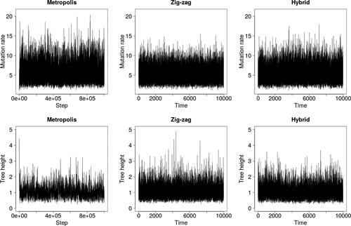
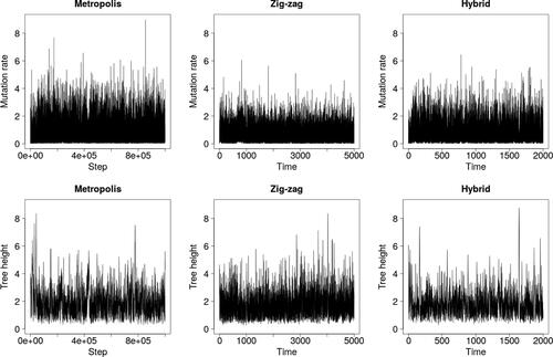
Figure 4 shows that the zig-zag and hybrid methods mix visibly better than Metropolis–Hastings over the latent tree, as measured by the tree height $H_n:=t_1+\cdots +t_{n-1}$. However, they are not as effective at exploring the upper tail of the θ-marginal, likely because they do not stay in regions of short trees for long enough for θ to increase into the tail.

Fig. 4 Trace plots under the infinite sites model and the dataset of Ward et al. (1991).

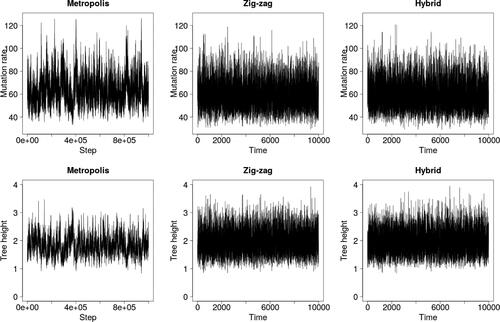
To assess scaling, we simulated two datasets: one of size n = 550 with mutation rate $\theta =5.5$ (the approximate posterior mean in Figure 4) and one with n = 55 and θ = 55, which models a segment of DNA 10 times longer. Figures 5 and 6 demonstrate that the zig-zag and hybrid processes scale far better than Metropolis–Hastings, particularly when θ = 55. Estimates in Table 1 quantify the improvement to 1–3 orders of magnitude.

Fig. 5 Trace plots for the infinite sites model and the dataset with n = 550, $\theta =5.5$, 30 distinct types, and 38 mutations.

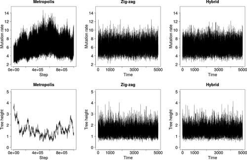
Fig. 6 Trace plots for the infinite sites model and the dataset with n = 55, θ = 55, 40 distinct types, and 252 mutations.

5 The Finite Sites Model

The finite sites model (Jukes and Cantor 1969) is more detailed than the infinite sites model, but has greater computational cost. Consider a finite set of sites S with a finite number of possible types H per site; for example $H=\{0,1\}$ or $H=\{A,T,C,G\}$. Mutations occur along branches of the coalescent tree at each site with rate $\theta /(2|S|)$, and the type of a mutant child is drawn from stochastic matrix P with unique stationary distribution ν. We denote the transition matrix of the H-valued compound Poisson process with jump rate $\theta /(2|S|)$ and jump transition matrix P by ${(Q_{hg}^{\theta }(t))}_{h,g\in H;t\ge 0}$. Figure 7 depicts a realization of the finite sites coalescent.

Fig. 7 A realization of the finite sites model with n = 4, $S=H=\{0,1\}$, three mutations, three types, and $D_n=(\#00,\#10,\#01,\#11)=(2,1,1,0)$.

As in Section 4, we denote the configuration of types at the leaves by D_n , and seek to sample from the posterior $\pi (E_n,{\mathbf{t}}_n,\theta |D_n)$, which can be written as a sum over the types of internal nodes:(16) $$\begin{array}{c}\pi (E_n,{\mathbf{t}}_n,\theta |D_n)\propto \{\prod _{s\in S}\sum _{\stackrel{h(s,c_{\gamma })\in H}{\text{for}\mathrm{ }\gamma \in F_n:\left|c_{\gamma }\right|>1}}\prod _{\gamma \in F_n}{Q}_{h(s;p_{\gamma })h(s;c_{\gamma })}^{\theta }(l_{\gamma })\}\\ \times \hspace{0.17em}\text{exp}\hspace{0.17em}(-\sum _{i=1}^{n-1}\left(\begin{array}{c}n+1-i\\ 2\end{array}\right)t_i){\pi }_0(\theta ),\end{array}$$(16) where $h(s;\eta )\in H$ is the type at site $s\in S$ on the node with label $\eta \in E_n$, and $\gamma \in F_n:\left|c_{\gamma }\right|>1$ denotes edges which do not end in a leaf. The target (16) can be evaluated efficiently using the pruning algorithm of Felsenstein (1981).

The posterior (16) can be sampled using zig-zag dynamics with the same construction as in Section 4. Velocity flip rates can be written in terms of branch-specific gradients as(17) $$\begin{array}{c}{\lambda }_i(E_n,{\mathbf{t}}_n,\theta ;{\mathbf{v}}_n)=[v_i(\left(\begin{array}{c}n+1-i\\ 2\end{array}\right)\\ -\sum _{s\in S}{\sum }_{\stackrel{h(s,c_{\gamma })\in H}{\mathrm{ }\text{for}\mathrm{ }\gamma \in F_n:\left|c_{\gamma }\right|>1}}{\sum }_{\delta \in F_n:t_i\in \delta }\\ \frac{[{\partial }_i{Q}_{h(s;p_{\delta })h(s;c_{\delta })}^{\theta }(l_{\delta })]\prod _{\gamma \in F_n:\gamma \ne \delta }{Q}_{h(s;p_{\gamma })h(s;c_{\gamma })}^{\theta }(l_{\gamma })}{\sum _{\stackrel{h(s,c_{\gamma })\in H}{\mathrm{ }\text{for}\mathrm{ }\gamma \in F_n:\left|c_{\gamma }\right|>1}}\prod _{\gamma \in F_n}{Q}_{h(s;p_{\gamma })h(s;c_{\gamma })}^{\theta }(l_{\gamma })}){]}^{+},\end{array}$$(17) (18) $$\begin{array}{c}{\lambda }_{\theta }(E_n,{\mathbf{t}}_n,\theta ;{\mathbf{v}}_n)=[-v_n({\partial }_{\theta }\hspace{0.17em}\text{log}\hspace{0.17em}({\pi }_0(\theta ))\\ +{\sum }_{s\in S}{\sum }_{\stackrel{h(s,c_{\gamma })\in H}{\mathrm{ }\text{for}\gamma \in F_n:\left|c_{\gamma }\right|>1}}{\sum }_{\delta \in F_n}\\ \frac{[{\partial }_{\theta }{Q}_{h(s;p_{\delta })h(s;c_{\delta })}^{\theta }(l_{\delta })]\prod _{\gamma \in F_n:\gamma \ne \delta }{Q}_{h(s;p_{\gamma })h(s;c_{\gamma })}^{\theta }(l_{\gamma })}{\sum _{\stackrel{h(s,c_{\gamma })\in H}{\mathrm{ }\text{for}\gamma \in F_n:\left|c_{\gamma }\right|>1}}\prod _{\gamma \in F_n}{Q}_{h(s;p_{\gamma })h(s;c_{\gamma })}^{\theta }(l_{\gamma })}){]}^{+},\end{array}$$(18) which can be evaluated using the linear-cost method of Ji et al. (2020).

We show that events with rates (17) and (18) can be simulated using the example of (Griffiths and Tavaré 1994, sec. 7.4), in which $S=\{1,\dots ,20\},H=\{0,1\}$ and P is the 2 × 2 matrix which always changes state, corresponding to $\nu =(1/2,1/2)$ and(19) $$\tilde{\pi }$$(19)

As (19) is not bounded away from 0 when $h\ne g$, (17) and (18) lack simple bounds for Poisson thinning. As in (15), bounds can be obtained by time localization using$$\begin{array}{c}T\equiv T(E_n,{\mathbf{t}}_n,\theta ;{\mathbf{v}}_n)\\ \hspace{1em}:=\min \left\{\underset{i\in \{1,\dots ,n\}:v_i<0}{\min }\right\{\frac{-t_i}{[1+c\mathrm{ }{1}_{\{1,\theta \}}(i)\mathrm{ }{1}_{{\mathbb{Z}}_{+}}(m_{\gamma (E_n,i)})]v_i}\},K\},\end{array}$$where $K\gg 0$ is a default increment in case all velocities are positive. The variable T localizes the next zig-zag time step beginning at time t so that at most one branch can shrink to length zero on $[t,t+T]$, θ can fall by at most $1/(1+c)$ of its present value, and t₁ can fall by at most $1/(1+c)$ of its present value if the first two leaves to merge are of distinct types. This treatment of θ and t₁ is needed as (17) and (18) diverge in these cases, rendering the θ = 0 and $t_1=0$ boundaries inaccessible.

Given $T\in (0,\infty )$, we have the following bounds on (19) on the time interval $[t,t+T]$:$$\begin{array}{cc}{Q}_{hh}^{\theta }(l_{\gamma })\hfill & \le \frac{1}{2}\{1+\hspace{0.17em}\text{exp}\hspace{0.17em}(-[\theta +{(v_{n}T)}^{-}][l_{\gamma }+{(v_{\gamma }T)}^{-}])\},\hfill \\ Q_{hg}^{\theta }(l_{\gamma })\hfill & \le \frac{1}{2}\{1-\hspace{0.17em}\text{exp}\hspace{0.17em}(-[\theta +{(v_{n}T)}^{+}][l_{\gamma }+{(v_{\gamma }T)}^{+}])\},\hfill \\ Q_{hh}^{\theta }(l_{\gamma })\hfill & \ge \frac{1}{2}\{1+\hspace{0.17em}\text{exp}\hspace{0.17em}(-[\theta +{(v_{n}T)}^{+}][l_{\gamma }+{(v_{\gamma }T)}^{+}])\},\hfill \\ Q_{hg}^{\theta }(l_{\gamma })\hfill & \ge \frac{1}{2}\{1-\hspace{0.17em}\text{exp}\hspace{0.17em}(-[\theta +{(v_{n}T)}^{-}][l_{\gamma }+{(v_{\gamma }T)}^{-}])\},\hfill \end{array}$$where $h\ne g$. Substituting these bounds into (Ji et al. 2020, eq. (9)(9) $$\pi (E_n,{\mathbf{t}}_n)\mathrm{d}{\mathbf{t}}_n:=\hspace{0.17em}\text{exp}\hspace{0.17em}(-\sum _{i=1}^{n-1}\left(\begin{array}{c}n+1-i\\ 2\end{array}\right)t_i)\mathrm{d}{\mathbf{t}}_n,$$(9) ) provides bounds on flip rates that can be evaluated with $O(|S|n)$ cost.

Figure 8 demonstrates that the zig-zag process again mixes over latent trees faster than Metropolis–Hastings, but struggles to explore the upper tail of the θ-marginal. The hybrid method was run with κ = 100 to compensate for shorter run lengths than in Section 4, and thus, resembles Metropolis–Hastings rather than the zig-zag process.

Fig. 8 Trace plots for the finite sites model and data from Griffiths and Tavaré (1994).

Figures 9 and 10 show results for two further simulated datasets: one with n = 500 and S = 20, and one with n = 50 and S = 200. The superior mixing of the zig-zag process over the latent tree is clear, as quantified by effective sample sizes in Table 2. The lack of mixing in the upper tail of the θ-marginal is also stark, particularly in Figure 9 where zig-zag significantly underestimates posterior variance. The estimated posterior means of all three methods coincide in all cases (results not shown).

Fig. 9 Trace plots for the finite sites model and dataset with n = 500 and S = 20 consisting of five distinct sequences.

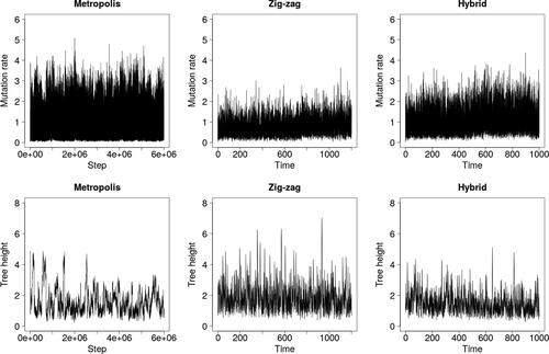
Fig. 10 Trace plots for the finite sites model and dataset with n = 50 and S = 200 consisting of 18 distinct sequences.

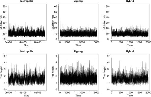
Table 2 Effective sample sizes and run times for all three methods and datasets.

Dataset	Method	ESS(θ)/sec	ESS(Hn)/sec	Run time (min)
Griffiths and Tavaré (1994)	Metropolis	1.8	0.2	29
	Zig-zag	2.3	1.0	18
	Hybrid	2.1	0.6	16
n = 500, S = 20	Metropolis	0.09	0.0006${}^{\ast }$	1567
	Zig-zag	0.01${}^{\ast }$	0.004	1749
	Hybrid	0.01	0.003	1800
n = 50, S = 200	Metropolis	0.04	0.03	257
	Zig-zag	0.05	0.13	175
	Hybrid	0.08	0.07	183

NOTE: Estimates were computed as in Table 1. Stars highlight unmixed chains with unreliable ESS estimates.

6 Discussion

We have presented a general method for using zig-zag processes to sample targets defined on hybrid spaces consisting of discrete and continuous variables. This was done by introducing boundaries into the state space of continuous variables and updating discrete components via a Markov jump kernel Q whenever a boundary was hit. The resulting algorithm remains a piecewise-deterministic Markov processes in the sense of (Davis 1993, sec. 24), and generalizes existing zig-zag processes for restricted domains (Bierkens et al. 2018). Crucially, no assumptions of structure among the discrete variables are required. The key conditions on Q are the skew-detailed balance (2), which is local, and (3), which involves an integral with respect to Q but not the target $\tilde{\pi }$. Both are verifiable in applications, and do not require $\tilde{\pi }$ to be normalized. Our method is reminiscent of discrete Hamiltonian Monte Carlo (Dinh et al. 2017; Nishimura, Dunson, and Lu 2020), but the lack of time discretization simplifies boundary crossings (though see Nishimura, Dunson, and Lu 2020, sec. S6.4).

We have demonstrated the method on two examples involving the coalescent, which is a gold-standard model in phylogenetics. It is defined on the space of binary trees consisting of discrete tree topologies and continuous branch lengths, which lacks a simple geometric structure, for example, a partial order or a tractable norm. We have also shown that the zig-zag process can improve mixing over trees relative to Metropolis-Hastings, particularly under the infinite sites model. This model is widely used to analyze ever larger datasets, and the zig-zag process shows promise for expanding the scope of feasible MCMC computations.

The zig-zag process was more efficient than Metropolis–Hastings under the infinite sites model in terms of effective sample size, but struggled to explore the tails of the θ-marginal. A likely reason is correlation in the target: high mutation rates are only be attainable when branch lengths are short. A Metropolis–Hastings algorithm can jump to a high mutation rate as soon as the latent tree has short branches, while the zig-zag process must traverse all intervening mutation rates before branch lengths grow. The speed up zig-zag method of Vasdekis and Roberts (2021) has state-dependent velocities, and could provide further improvement. The hybrid method with both zig-zag motion and Metropolis-Hastings updates interpolated between the two algorithms.

All three algorithms exhibited much longer run times under the finite sites model than under infinite sites. For the zig-zag and hybrid methods, that is due to the $O(|S|n)$ cost per evaluation of (17) and (18), of which there are O(n). However, flip times for different velocities are conditionally independent given the current state and can be generated in parallel, unlike steps of the Metropolis–Hastings algorithm. Hence, the zig-zag process is well suited to parallel architectures.

Acknowledgments

The author is grateful to Jure Vogrinc and Andi Wang for productive conversations on MCMC for coalescent processes, and nonreversible MCMC in general.

Supplementary Materials

The supplementary materials contains the proofs of Theorem 1 and Proposition 1, as well as details of the zig-zag and Metropolis–Hastings algorithms used in Sections 4 and 5.

Additional information

Funding

The author was supported by ESPRC grant EP/R044732/1.

References

- Aberer, A. J., Stamatakis, A., and Ronquist, F. (2016), “An Efficient Independence Sampler for Updating Branches in Bayesian Markov Chain Monte Carlo Sampling of Phylogenetic Trees,” Systematic Biology, 65, 161–176. DOI: 10.1093/sysbio/syv051.
- Bierkens, J., Bouchard-Côte, A., Doucet, A., Duncan, A. B., Fearnhead, P., Lienart, T., Roberts, G., and Vollmer, S. J. (2018), “Piecewise Deterministic Markov Processes for Scalable Monte Carlo on Restricted Domains,” Statistics & Probability Letters, 136, 148–154.
- Bierkens, J., Fearnhead, P., and Roberts, G. (2019a), “Supplement to ‘The Zig-zag Process and Super-Efficient Sampling for Bayesian Analysis of Big Data’,” Annals of Statistics, 47.
- Bierkens, J., Fearnhead, P., and Roberts, G. (2019b), “The Zig-zag Process and Super-Efficient Sampling for Bayesian Analysis of Big Data,” Annals of Statistics, 47, 1288–1320.
- Bierkens, J., and Roberts, G. (2017), “A Piecewise Deterministic Scaling Limit of Lifted Metropolis-Hastings for the Curie-Weiss Model,” Annals of Applied Probability, 27, 846–882.
- Bierkens, J., Roberts, G., and Zitt, P.-A. (2019), “Ergodicity of the Zigzag Process,” Annals of Applied Probability, 29, 2266–2301.
- Billera, L. J., Holmes, S. P., and Vogtmann, K. (2001), “Geometry of the Space of Phylogenetic Trees,” Advances in Applied Mathematics, 27, 733–767. DOI: 10.1006/aama.2001.0759.
- Chevalier, A., Fearnhead, P., and Sutton, M. (2020), “Reversible Jump PDMP Samplers for Variable Selection,” preprint, arXiv:2010.11771.
- Davis, M. (1993), Markov Models and Optimization, Boca Raton, FL: Chapman Hall.
- Dinh, V., Bilge, A., Zhang, C., and Matsen, F. A., IV. (2017), “Probabilistic Path Hamiltonian Monte Carlo,” in Proceedings of the 34th International Conference on Machine Learning, Sydney, Australia.
- Felsenstein, J. (1981), “Evolutionary Trees from DNA Sequences: A Maximum Likelihood Approach,” Journal of Molecular Evolution, 17, 368–376. DOI: 10.1007/BF01734359.
- Flegal, J. M., Hughes, J., Vats, D., and Dai, N. (2017), mcmcse: Monte Carlo Standard Errors for MCMC.
- Gagnon, P., and Doucet, A. (2021), “Nonreversible Jump Algorithms for Bayesian Nested Model Selection,” Journal of Computational and Graphical Statistics, 30, 312–323. DOI: 10.1080/10618600.2020.1826955.
- Gavryushkin, A., and Drummond, A. J. (2016), “The Space of Ultrametric Phylogenetic Trees,” Journal of Theoretical Biology, 403, 197–208. DOI: 10.1016/j.jtbi.2016.05.001.
- Gelfand, A. E., and Smith, A. F. M. (1990), “Sampling-Based Approaches to Calculating Marginal Densities,” Journal of the American Statistical Association, 85, 398–409. DOI: 10.1080/01621459.1990.10476213.
- Geyer, C. J. (1992), “Practical Markov Chain Monte Carlo,” Statistical Science, 7, 473–483. DOI: 10.1214/ss/1177011137.
- Griffiths, R. C., and Tavaré, S. (1994), “Simulating Probability Distributions in the Coalescent,” Theoretical Population Biology, 46, 131–159. DOI: 10.1006/tpbi.1994.1023.
- Hastings, W. K. (1970), “Monte Carlo Sampling Methods Using Markov Chains and their Applications,” Biometrika, 57, 97–109. DOI: 10.1093/biomet/57.1.97.
- Höhna, S., Defoin-Platel, M., and Drummond, A. J. (2008), “Clock-Constrained Tree Proposal Operators in Bayesian Phylogenetic Inference,” in 8th IEEE International Conference on BioInformatics and BioEngineering, pp. 1–7.
- Höhna, S., and Drummond, A. J. (2012), “Guided Tree Topology Proposals for Bayesian Phylogenetic Inference, Systematic Biology, 61, 1–11. DOI: 10.1093/sysbio/syr074.
- Ji, X., Zhang, Z., Holbrook, A., Nishimura, A., Baele, G., Rambaut,A., Lemey, P., and Suchard, M. A. (2020), “Gradients Do Grow on Trees: A Linear-time O(N)-Dimensional Gradient for Statistical Phylogenetics,” Molecular Biology and Evolution, 37, 3047–3060. DOI: 10.1093/molbev/msaa130.
- Jukes, T. H., and Cantor, C. R. (1969), “Evolution of Protein Molecules,” in Mammalian protein metabolism, ed. H. N. Munro, pp. 21–132, New York: Academic Press.
- Kingman, J. F. C. (1982), “The Coalescent,” Stochastic Processes and Their Applications, 13, 235–248. DOI: 10.1016/0304-4149(82)90011-4.
- Lakner, C., Van Der Mark, P., Huelsenbeck, J. P., Larget, B., and Ronquist, F. (2008), “Efficiency of Markov Chain Monte Carlo Tree Proposals in Bayesian Phylogenetics,” Systematic Biology, 57, 86–103. DOI: 10.1080/10635150801886156.
- Mossel, E., and Vigoda, E. (2005), “Phylogenetic MCMC Algorithms are Misleading on Mixtures of Trees,” Science, 309, 2207–2209. DOI: 10.1126/science.1115493.
- Neal, R. M. (2010), “MCMC Using Hamiltonian Dynamics,” in Handbook of Markov Chain Monte Carlo, S. Brooks, A. Gelman, G. Jones, and X.-L. Meng, Boca Raton, FL: CRC Press.
- Nishimura, A., Dunson, D. B., and Lu, J. (2020), “Discontinuous Hamiltonian Monte Carlo for Discrete Parameters and Discontinuous Likelihoods,” Biometrika, 107, 365–380. DOI: 10.1093/biomet/asz083.
- Vasdekis, G., and Roberts, G. O. (2021), “Speed Up Zig-zag,” preprint, arXiv:2103.16620.
- Wakeley, J. (2009), Coalescent Theory: An Introduction, Greenwood Village, CO: Roberts & Co.
- Ward, R. H., Frazier, B. L., Dew, K., and Pääbo, S. (1991), “Extensive Mitochondrial Diversity Within a Single Amerindian Tribe,” Proceedings of the National Academy of Sciences of the United States of America, 88, 8720–8724. DOI: 10.1073/pnas.88.19.8720.
- Watterson, G. A. (1975), “On the Number of Segregating Sites in Genetical Models Without Recombination,” Theoretical Population Biology, 7, 256–276. DOI: 10.1016/0040-5809(75)90020-9.