A Simple Algorithm for Exact Multinomial Tests

Abstract

This work proposes a new method for computing acceptance regions of exact multinomial tests. From this an algorithm is derived, which finds exact p-values for tests of simple multinomial hypotheses. Using concepts from discrete convex analysis, the method is proven to be exact for various popular test statistics, including Pearson’s Chi-square and the log-likelihood ratio. The proposed algorithm improves greatly on the naive approach using full enumeration of the sample space. However, its use is limited to multinomial distributions with a small number of categories, as the runtime grows exponentially in the number of possible outcomes. The method is applied in a simulation study, and uses of multinomial tests in forecast evaluation are outlined. Additionally, properties of a test statistic using probability ordering, referred to as the “exact multinomial test” by some authors, are investigated and discussed. The algorithm is implemented in the accompanying R package ExactMultinom. Supplementary materials for this article are available online.

Keywords:

• Acceptance regions
• Goodness-of-fit test
• Log-likelihood ratio
• Pearson’s Chi-square
• Probability mass statistic
• R software

1 Introduction

Multinomial goodness-of-fit tests feature prominently in the statistical literature and a wide range of applications. Tests relying on asymptotics have been available for a long time and have been rigorously studied all through the 20th century. The use of various test statistics has been investigated with Pearson’s Chi-square and the log-likelihood ratio statistic being vital examples. These statistics are members of the general family of power divergence statistics (Cressie and Read 1984). With the widespread availability of computing power, Monte Carlo simulations and exact methods have also gained popularity.

Tate and Hyer (1973) and Kotze and Gokhale (1980) used the “exact multinomial test,” which orders samples by probability, to assess the accuracy of asymptotic tests of a simple null hypothesis against an unspecified alternative. In the words of Cressie and Read (1989), this “has provided much confusion and contention in the literature.” In accordance with Gibbons and Pratt (1975) and Radlow and Alf (1975), they conclude that the asymptotic fit of a test should be assessed using the appropriate exact test based on the test statistic in question. Nevertheless, the exact multinomial test is intuitively appealing, and, as Kotze and Gokhale (1980) put it, “[i]n the absence of […] a specific alternative, it is reasonable to assume that outcomes with smaller probabilities under the null hypothesis offer a stronger evidence for its rejection and should belong to the critical region.” In Section 2, an asymptotic Chi-square approximation to the exact multinomial test is derived, and an exemplary comparison of popular test statistics in terms of power is provided.

Regardless of the test statistic used, computing an exact p-value by fully enumerating the sample space is computationally challenging, as the test statistic and the probability mass function have to be evaluated at every possible sample of which there are $\left(\begin{array}{c}n+m-1\\ m-1\end{array}\right)=\mathcal{O}(n^{m-1})$ for samples of size n with m categories. An improvement on this method has been proposed by Bejerano, Friedman, and Tishby (2004) for the family of power divergence statistics. Other approaches aimed at exact Pearson’s Chi-square and log-likelihood ratio tests exist (see, e.g., Baglivo, Olivier, and Pagano 1992; Hirji 1997; Rahmann 2003; Keich and Nagarajan 2006). In this work, a new approach to exact multinomial tests is investigated.

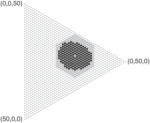
The key observation underlying the proposed algorithm is that acceptance regions at arbitrary levels contain relatively few points, which are located in a neighborhood of the expected value under the null hypothesis as illustrated in Figure 1, and an acceptance region can be found by iteratively evaluating points within a ball of increasing radius around the expected value (w.r.t. the Manhattan distance). The algorithm uses this to compute an exact p-value from the probability mass of the largest acceptance region that does not contain the observation. If p-values below an arbitrary threshold are not computed exactly, the runtime of the algorithm is guaranteed to be asymptotically faster than the approach using full enumeration as the diameter of any acceptance region essentially grows at a rate proportional to the square root of the sample size. This is detailed and proven to work for various popular test statistics in Section 3.

Fig. 1 An acceptance region (black dots) at level $\alpha =0.05$ for the null $\pi =(\frac{2}{10},\frac{5}{10},\frac{3}{10})$ and samples of size n = 50 with m = 3 categories. Only points within the ball (big dots) around the expectation (hollow dot) have to be considered to find this region.

Furthermore, the algorithm is illustrated to work well in applications detailed in Section 4. In particular, the algorithm’s runtime is compared to the full enumeration method in a simulation study, and the resulting p-values are used to assess the fit of asymptotic Chi-square approximations and investigate differences between several test statistics. As an application in forecast evaluation, the use of multinomial tests for uncertainty quantification within the so-called calibration simplex (Wilks 2013) is outlined and justified.

The R programming language (R Core Team 2020) has been used for all computations throughout this work. An implementation of the proposed method is provided within the R package ExactMultinom (Resin 2020).

2 A Brief Review on Testing a Simple Multinomial Hypothesis

Consider a multinomial experiment $X=(X_1,\dots ,X_m)$ summarizing $n\in \mathbb{N}$ iid trials with $m\in \mathbb{N}$ possible outcomes. Let$${\Delta }_{m-1}:=\{p\in {[0,1]}^m|p_1+\cdots +p_m=1\}$$denote the unit $(m-1)$-simplex or probability simplex and$${\Omega }_{m,n}=\{x\in {\mathbb{N}}_0^m|x_1+\cdots +x_m=n\}$$ the sample space, which is a regular discrete $(m-1)$-simplex. The distribution of X is characterized by a parameter $p=(p_1,\dots ,p_m)\in {\Delta }_{m-1}$ encoding the occurrence probabilities of the outcomes on any trial, or $X\sim {\mathcal{M}}_m(n,p)$ for short. The multinomial distribution ${\mathcal{M}}_m(n,p)$ is fully described by the probability mass function (pmf)$$f_{n,p}:{\Omega }_{m,n}\to [0,1],x\mapsto n!\prod _{j=1}^m\frac{p_j^{x_j}}{x_j!}.$$

Suppose that the true parameter p is unknown. Consider the simple null hypothesis $p=\pi$ for some $\pi \in {\Delta }_{m-1}$. The agreement of a realization $x\in {\Omega }_{m,n}$ of X with the null hypothesis is typically quantified by means of a test statistic $T:{\Omega }_{m,n}\times {\Delta }_{m-1}\to ℝ$. Given such a test statistic T and presuming from now on that w.l.o.g. high values of $T(x,\pi )$ indicate “extreme” observations under the null distribution ${\mathrm{\mathbb{P}}}_{\pi }$, the p-value of x is defined as the probability(1) $$p_T(x,\pi ):={\mathrm{\mathbb{P}}}_{\pi }(T(X,\pi )\ge T(x,\pi ))$$(1) of observing an observation that is at least as extreme under the null hypothesis.

The family of power divergence statistics introduced by Cressie and Read (1984) offers a variety of test statistics for multinomial goodness-of-fit tests. It is defined as(2) $$\begin{array}{c}{T}^{\lambda }(x,\pi ):=\frac{2}{\lambda (\lambda +1)}\sum _{j=1}^m{x}_j\left({\left(\mathrm{}\frac{x_j}{n{\pi }_j}\right)}^{\lambda }-1\mathrm{}\right)\\ \text{for}\mathrm{ }\lambda \in ℝ\mathrm{\setminus }\{-1,0\}\end{array}$$(2) and as the pointwise limit in (2) for $\lambda \in \{-1,0\}$. Notably, this includes Pearson’s Chi-square statistic$$T^{{\chi }^2}(x,\pi ):=\sum _{j=1}^m\frac{{(x_j-n{\pi }_j)}^2}{n{\pi }_j}=\sum _{j=1}^m\frac{x_j^2}{n{\pi }_j}-n=T^1(x,\pi )$$ as well as the log-likelihood ratio (or G-test) statistic$$T^G(x,\pi ):=2\hspace{0.17em}\text{log}\hspace{0.17em}\frac{f_{n,\frac{x}{n}}(x)}{f_{n,\pi }(x)}=2\sum _{j=1}^m{x}_j\hspace{0.17em}\text{log}\hspace{0.17em}\frac{x_j}{n{\pi }_j}=T^0(x,\pi ).$$

Under a null hypothesis with ${\pi }_i>0$ for all $i=1,\dots ,m$, every power divergence statistic is asymptotically Chi-square distributed with m – 1 degrees of freedom.

A natural test statistic arises if an “extreme” observation is simply understood to mean an unlikely one, that is, if the pmf itself is used as test statistic. In what follows, a strictly decreasing transformation of the pmf is used instead, which ensures that large values of the test statistic indicate extreme observations. Furthermore, this strictly decreasing transformation is chosen such that the resulting test statistic is asymptotically Chi-square distributed. To this end, let Γ denote the Gamma function and$${\overline{f}}_{n,p}:\{x\in {ℝ}_{\ge 0}^m|x_1+\cdots +x_m=n\}\to ℝ,x\mapsto \Gamma (n+1)\prod _{j=1}^m\frac{p_j^{x_j}}{\Gamma (x_j+1)}$$the continuous extension of the pmf $f_{n,p}$ to the convex hull of the discrete simplex ${\Omega }_{m,n}$. The probability mass test statistic is defined as$$T^{\mathrm{\mathbb{P}}}(x,\pi ):=-2\hspace{0.17em}\text{log}\hspace{0.17em}\frac{f_{n,\pi }(x)}{{\overline{f}}_{n,\pi }(n\pi )}.$$

Obviously, the choice of strictly decreasing transformation does not affect the (exact) p-value given by (1) for $T=T^{\mathrm{\mathbb{P}}}$. The following theorem gives rise to an asymptotic approximation of p-values derived from the probability mass test statistic, which has not been studied previously. In the simulation study of Section 4, the fit of this approximation is assessed empirically using exact p-values computed with the new method for samples of size n = 100 with m = 5 categories.

Theorem 1.

If $X\sim {\mathcal{M}}_m(n,\pi )$ follows a multinomial distribution with $n\in \mathbb{N}$ and $\pi \in {\Delta }_{m-1}$ such that ${\pi }_j>0$ for $j=1,\dots ,m$, then $T^{\mathrm{\mathbb{P}}}(X,\pi )$ converges in distribution to a Chi-square distribution ${\chi }_{m-1}^2$ with m – 1 degrees of freedom as $n\to \infty$.

Proof.

By Lemma 8 (in Appendix A, supplementary materials), the difference between the log-likelihood ratio and the probability mass statistic is$$T^{\mathrm{\mathbb{P}}}(X,\pi )-T^G(X,\pi )=\sum _{j=1}^m\left(\hspace{0.17em}\text{log}\hspace{0.17em}\frac{X_j}{n{\pi }_j}+\mathcal{O}(1/X_j)-\mathcal{O}(1/n)\right).$$

Clearly, the bounded terms converge to zero in probability, and the $\text{log}\hspace{0.17em}\frac{X_j}{n{\pi }_j}$ terms converge to zero in probability by the continuous mapping theorem. Hence, the probability mass statistic has the same asymptotic distribution as the log-likelihood ratio statistic. □

In what follows, the focus is on the Chi-square, log-likelihood ratio and probability mass statistics.

2.1 Acceptance Regions

As outlined in the introduction, acceptance regions are of major importance to the idea pursued in this work. Given a test statistic T, the acceptance region at level $\alpha >0$ is defined using p-values given by (1) as$$A_{n,\pi }^T(\alpha ):=\{x\in {\Omega }_{m,n}|p_T(x,\pi )>\alpha \}.$$

Equivalently, the acceptance region can be written as the sublevel set of $T(·,\pi )$ at the $(1-\alpha )$-quantile $t_{1-\alpha }=\min \{t\in ℝ|{\mathrm{\mathbb{P}}}_{\pi }(T(X,\pi )\le t)\ge 1-\alpha \}$ of $T(X,\pi )$ under the null hypothesis $X\sim {\mathcal{M}}_m(n,\pi )$, that is,(3) $$A_{n,\pi }^T(\alpha )=\{x\in {\Omega }_{m,n}|T(x,\pi )\le t_{1-\alpha }\}.$$(3)

As illustrated in Figure 2, the probability mass test statistic typically yields acceptance regions that contain relatively few points, because the regions contain the samples with the largest null probabilities. However, as samples with equal null probabilities are either all included or all excluded, smaller acceptance regions might be feasible at some levels α. If tests are randomized to ensure equal level and size of the test, this property can be refined to yield an optimality property of the probability mass test’s critical function.

Fig. 2 Acceptance regions (black) of probability mass (left), Chi-square (center) and log-likelihood ratio (right) statistics at level $\alpha =0.05$ for n = 50 and $\pi =(\frac{1}{10},\frac{7}{10},\frac{2}{10})$. The regions contain 108, 111, and 111 points, respectively (left to right). The tests are of size 0.0495, 0.0492, and 0.0481, respectively.

In Section 3, it is shown that acceptance regions of the Chi-square, log-likelihood ratio and probability mass test statistic all grow at a rate $\mathcal{O}\left(n^{\frac{m-1}{2}}\right)$, as their diameter grows at a rate $\mathcal{O}\left(\sqrt{n}\right)$ if $\alpha >0$ is fixed, see Proposition 7.

2.2 Power and Bias

The power function of a test T of the null hypothesis $p=\pi$ at level α is$${\Delta }_{m-1}\to [0,1],p\mapsto 1-{\mathrm{\mathbb{P}}}_p(T(X)\in A_{n,\pi }^T(\alpha )),$$which is the probability of rejecting the null hypothesis at level α if the true parameter is p. The size of a test is its power at $p=\pi$. A test T is said to be unbiased (for the null $p=\pi$ at level α) if its power is minimized at $p=\pi$.

In the case of the uniform null hypothesis, that is, $\pi =(\frac{1}{m},\dots ,\frac{1}{m})$, Cohen and Sackrowitz (1975, Theorem 2.1) proved that the power function increases away from $p=\pi$ for test statistics of the form$$T(x)=\sum _{j=1}^{m}h(x_j)$$if h is a convex function. They concluded that tests based on the Chi-square and the log-likelihood ratio test statistic are unbiased for the uniform null hypothesis. As a corollary to their theorem, it shall be noted that this also applies to the probability mass test statistic.

Corollary 2

(to Cohen and Sackrowitz 1975, Theorem 2.1). The probability mass test is unbiased for the uniform null hypothesis $p=\pi =(\frac{1}{m},\dots ,\frac{1}{m})$.

Proof.

Since the probability mass statistic can be written as$$T^{\mathrm{\mathbb{P}}}(x,\pi )=2\sum _{j=1}^m\hspace{0.17em}\text{log}\hspace{0.17em}\Gamma (x_j+1)-x_j\hspace{0.17em}\text{log}\hspace{0.17em}{\pi }_j-\hspace{0.17em}\text{log}\hspace{0.17em}\frac{\Gamma (n{\pi }_j+1)}{{\pi }_j^{n{\pi }_j}},$$this is an immediate consequence of the fact that the Gamma function is logarithmically convex on the positive real numbers, which is part of a characterization given by the Bohr-Mollerup theorem (Beals and Wong 2010, Theorem 2.4.2). □

Many authors (e.g., West and Kempthorne 1972; Cressie and Read 1984; Wakimoto, Odaka, and Kang 1987; Pérez and Pardo 2003) have conducted small sample studies to investigate the power of Chi-square, log-likelihood ratio and other tests. When conducting such studies, $\pi ,n$, and α need to be chosen, all of which influence the resulting power function. Furthermore, it is frequently infeasible to assess the power function across all alternatives, and so alternatives of interest need to be picked. Therefore, most of these studies focused on the case of the uniform null hypothesis. In this case, the Chi-square test has greater power for alternatives that assign a large proportion of the probability mass to relatively few categories, whereas the log-likelihood ratio test has greater power for alternatives that assign considerable probability mass to many categories (see also Koehler and Larntz 1980).

In the ternary case, that is, if m = 3, comparisons on the full probability simplex are visually accessible. Figure 3 illustrates, which of the three test statistics yields the highest and lowest power across the full ternary probability simplex. As the actual test size, which is frequently smaller than the level α, depends on the test statistic, the resulting power functions are difficult to compare directly. To account for this, the tests are randomized to ensure that their respective size matches the level. For a test T and level α, let $s_{n,\pi }(T,\alpha )=1-{\mathrm{\mathbb{P}}}_{\pi }(T(X)\in A_{n,\pi }^T(\alpha ))$ denote the actual size of the test. The critical function $$\varphi :{\Omega }_{m,n}\to [0,1],x\mapsto \{\begin{array}{cc}0,\hfill & \text{if}\mathrm{ }T(x,\pi )<t_{1-\alpha },\hfill \\ \frac{\alpha -s_{n,\pi }(T,\alpha )}{{\mathrm{\mathbb{P}}}_{\pi }(T(X)=t_{1-\alpha })},\hfill & \text{if}\mathrm{ }T(x,\pi )=t_{1-\alpha },\hfill \\ 1,\hfill & \text{if}\mathrm{ }T(x,\pi )>t_{1-\alpha },\hfill \end{array}$$defines a randomized test,¹ which rejects the null hypothesis with probability $\varphi (x)$ if x is observed. The power function of the randomized version of a test T at level α is$$p\mapsto \sum _{x\in {\Omega }_{m,n}}\varphi (x){\mathrm{\mathbb{P}}}_p(X=x)=1-\sum _{x\in A_{n,\pi }^T(\alpha )}(1-\varphi (x)){\mathrm{\mathbb{P}}}_p(X=x).$$

Fig. 3 Ternary plots indicating which randomized tests of size $\alpha =0.05$ yields the highest (left) and lowest (right) power for the uniform null hypothesis $\pi =(\frac{1}{3},\frac{1}{3},\frac{1}{3})$ (top) and $\pi =(\frac{1}{10},\frac{7}{10},\frac{2}{10})$ (bottom) for n = 50. Overlapping lines indicate nearly equal powers ($\text{difference}<{10}^{-5}$).

With this, the probability mass test minimizes the acceptance region in the sense that it minimizes the sum$$\sum _{x\in {\Omega }_{m,n}}(1-\varphi (x))$$across all randomized tests $\varphi$ with $\sum _x\varphi (x)f_{n,\pi }(x)=\alpha$.

Figure 3 suggests that the probability mass test and the log-likelihood ratio test for the uniform null hypothesis at level $\alpha =0.05$ are the same for n = 50. This is a coincidence, and for other choices of α (e.g., $\alpha =0.13$, for which coincidentally the probability mass statistic yields the same acceptance region as the Chi-square statistic) the acceptance regions differ, and so do the power functions.

Figure 4 quantitatively compares power along alternatives of the form$$\begin{array}{c}p(q,i)=(\tilde{q}{\pi }_1,\dots ,\tilde{q}{\pi }_{i-1},q,\tilde{q}{\pi }_{i+1},\dots ,\tilde{q}{\pi }_m)\in {\Delta }_{m-1}\\ \hspace{1em}\text{with}\mathrm{ }\tilde{q}=\frac{1-q}{1-{\pi }_i}\end{array}$$for $i=1,\dots ,m$ and $q\in [0,1]$. This yields parameterizations of the lines through π and a corner of the probability simplex. The figures illustrate that in the case $n=50,\pi =(\frac{1}{10},\frac{7}{10},\frac{2}{10})$ and $\alpha =0.05$, the log-likelihood ratio test, arguably, does not show any visible bias, whereas the Chi-square test shows the most bias. The power function of the probability mass test lies in between the other power functions across most of the probability simplex, and so the probability mass test might serve as a good compromise in terms of power.

Fig. 4 Power functions of randomized tests of size $\alpha =0.05$ along alternatives given by $p(p_i,i),i=1,2,3$ with null hypothesis $\pi =(\frac{1}{10},\frac{7}{10},\frac{2}{10})$ and sample size n = 50.

3 Exact p-Values via Acceptance Regions

Throughout this section, T is a test statistic, and $m,n\in \mathbb{N}$ and $\pi \in {\Delta }_{m-1}$ are fixed. To ease notation, the subscripts in the pmf of the null distribution are omitted, that is, $f=f_{n,\pi }$ and the test statistic T is considered as a function on the sample space only, that is, $T(·)=T(·,\pi )$. Let$$d:{ℝ}^m\times {ℝ}^m\to {ℝ}_{\ge 0},(x,y)\mapsto \frac{1}{2}\left|\right|x-y|{|}_1=\frac{1}{2}\sum _j|x_j-y_j|$$be a rescaled version of the Manhattan distance and$$B_r(y)=\{x\in {\Omega }_{m,n}|d(x,y)\le r\}$$ the discrete ball with radius $r\in \mathbb{N}$ and center $y\in {\Omega }_{m,n}$. Furthermore, $e_i={({\delta }_{ij})}_{j=1}^m$ denotes the ith vector of the standard basis of ${ℝ}^m$, where δ_ij is the Kronecker delta.

3.1 Finding Acceptance Regions Using Discrete Convex Analysis

As alluded to in the introduction, an acceptance region $A=A_{n,\pi }^T(\alpha )$ for $\alpha \in (0,1)$ can be found without enumerating all points of the sample space ${\Omega }_{m,n}$, but only considering points in some ball around the expected value for many test statistics. Specifically, if T is weakly quasi M-convex, that is, if for all distinct $x,y\in {\Omega }_{m,n}$ there exist indices $i,j\in \{1,\dots ,m\}$ such that $x_i>y_i,x_j<y_j$ and$$T(x-e_i+e_j)\le T(x)\hspace{1em}\mathrm{ }\text{or}\mathrm{ }\hspace{1em}T(y+e_i-e_j)\le T(y),$$the following theorem, which is proven at the end of this section, holds.

Theorem 3.

Let T be weakly quasi M-convex, and suppose $y\in {\Omega }_{m,n},r\in \mathbb{N}$ and $\alpha \in (0,1)$ are such that $\sum _{x\in B_r(y)}f(x)\ge 1-\alpha$. Let $t\in ℝ$ be the smallest level such that the sublevel set $A=\{x\in B_r(y)|T(x)\le t\}$ satisfies $\sum _{x\in A}f(x)\ge 1-\alpha$. If $A\subseteq B_{r-1}(y)$, then A is the acceptance region $A_{n,\pi }^T(\alpha )$.

Hence, an acceptance region can be found by iteratively enumerating a ball of increasing radius with arbitrary center until a sublevel set with enough probability mass is found and this sublevel set remains unchanged upon further increasing the ball, as illustrated in the introduction for an acceptance region of the probability mass statistic, see Figure 1.

The following proposition ensures that this approach can be applied to the Chi-square, log-likelihood ratio and probability mass test statistics.

Proposition 4.

1. The probability mass test statistic $T^{\mathrm{\mathbb{P}}}$ is weakly quasi M-convex.

2. The power divergence test statistic $T^{\lambda }$ is weakly quasi M-convex if $\lambda \ge 0$.

Proof.

Throughout the proof, let $x,y\in {\Omega }_{m,n}$ such that $x\ne y$, and define the index sets$$S^{+}:=\left\{i\right|x_i>y_i\}\hspace{1em}\mathrm{ }\text{and}\mathrm{ }\hspace{1em}{S}^{-}:=\{j|x_j<y_j\}.$$

1. Let $T=T^{\mathrm{\mathbb{P}}}$ and w.l.o.g. $T(x)\ge T(y)$. Then$$\begin{array}{c}T(y)-T(x)=-2\hspace{0.17em}\text{log}\hspace{0.17em}\frac{f(y)}{f(x)}\\ =-2\hspace{0.17em}\text{log}\hspace{0.17em}\left(\prod _{i\in S^{+}}\frac{x_i!}{y_i!}{\pi }_i^{y_i-x_i}·\prod _{j\in S^{-}}\frac{x_j!}{y_j!}{\pi }_j^{y_j-x_j}\mathrm{}\right)\\ =-2\hspace{0.17em}\text{log}\hspace{0.17em}\mathrm{}\left(\prod _{i\in S^{+}}\prod _{k=1}^{x_i-y_i}\frac{y_i+k}{{\pi }_i}·\prod _{j\in S^{-}}\prod _{k=1}^{y_j-x_j}\frac{{\pi }_j}{x_j+k}\mathrm{}\right)\le 0.\end{array}$$

Both double products contain an equal number of multiplicands (since $\sum _j{x}_j=\sum _j{y}_j=n$) and are nonempty (since $x\ne y$). As the entire product is at least 1, there exist indices $i\in S^{+}$ and $j\in S^{-}$ and natural numbers $k^{+}\le x_i-y_i$ and $k^{-}\le y_j-x_j$ such that the second inequality holds in$$\frac{{\pi }_j}{x_j+1}\ge \frac{{\pi }_j}{x_j+k^{-}}\ge \frac{{\pi }_i}{y_i+k^{+}}\ge \frac{{\pi }_i}{x_i}.$$

Therefore, the inequality$$T(x-e_i+e_j)=T(x)-2\hspace{0.17em}\text{log}\hspace{0.17em}\left(\frac{x_i}{{\pi }_i}·\frac{{\pi }_j}{x_j+1}\right)\le T(x)$$

holds.

1. See Appendix B, supplementary materials.

The rest of this section is devoted to the proof of Theorem 3, which uses the existence of certain sequences in the sublevel sets of weakly quasi M-convex functions given by the first part of the following lemma. It can be shown that the existence of such sequences characterizes a “weakly quasi M-convex set.” For further details on weak quasi M-convexity and discrete convex analysis in general, see Murota (2003).

Lemma 5.

Let T be a weakly quasi M-convex function and $L=\{x\in {\Omega }_{m,n}|T(x)\le t\}$ be the sublevel set of T at $t\in ℝ$.

1. If $x,y\in L$ and $d=d(x,y)$, then there exists a sequence $x_0,x_1,\dots ,x_d\in L$ with $x_0=x$, x_d = y and $d(x_i,x_{i+1})=1$ for all $i=0,1,\dots ,d-1$.

2. Suppose $y\in {\Omega }_{m,n}$ and $r\in \mathbb{N}$ are such that $A=\{x\in B_r(y)|T(x)\le t\}$ is not empty. If $A\subseteq B_{r-1}(y)$, then A = L is the sublevel set of T at t.

Proof.

1. Proof by induction on d: Let $x,y\in L$ and $d=d(x,y)$. If d = 0, then $x=x_0=y$ satisfies the condition. If d > 0, there exist i, j such that $x_i>y_i,x_j<y_j$ and $x_{d-1}=y+e_i-e_j\in L$ (or $x_{d-1}=x-e_i+e_j\in L$, in which case interchanging x and y and i and j yields the former formula for $x_{d-1}$) by weak quasi M-convexity of T. Then $d(x_{d-1},y)=1$ and$$\begin{array}{c}d(x,x_{d-1})=\frac{1}{2}(\sum _{k\ne i,j}|x_k-y_k|+\underset{=|x_i-y_i|-1}{\underbrace{|x_i-(y_i+1)|}}+\underset{=|x_j-y_j|-1}{\underbrace{|x_j-(y_j-1)|}})\\ =\frac{1}{2}(||x-y|{|}_1-2)=d-1.\end{array}$$

   By induction hypothesis, there exists a sequence $x_0,x_1,\dots ,x_{d-1}\in L$, such that $x=x_0,x_1,\dots ,x_{d-1},x_d=y\in L$ is the sought-after sequence.

2. Assume there exists some $b\in L\mathrm{\setminus }A$ and fix $a\in A$. By part a), the sublevel set L contains a sequence $a=x_0,x_1,\dots ,x_d=b\in L$ with $d=d(a,b)$ and $d(x_i,x_{i+1})=1$ for $i=0,1,\dots ,d-1$. By the reverse triangle inequality $|d(x_{i+1},y)-d(x_i,y)|\le 1$, and, since $d(a,y)<r<d(b,y)$, there is an x_j such that $d(x_j,y)=r$, which yields $x_j\in A$, a contradiction (as $A\subseteq B_{r-1}(y)$). Therefore, $L\subseteq A$, and hence A = L.

With this, the theorem is readily proven as follows.

Proof of Theorem 3.

Let $t\in ℝ$ be minimal such that $A=\{x\in B_r(y)|T(x)\le t\}$ has probability mass $\sum _{x\in A}f(x)\ge 1-\alpha$ and $A\subseteq B_{r-1}(y)$. Recall that the acceptance region $A_{n,\pi }^T(\alpha )$ is the sublevel set (3) at $t_{1-\alpha }$, and note that $t_{1-\alpha }\le t$ holds, as ${\mathrm{\mathbb{P}}}_{\pi }(T(X)\le t)\ge \sum _{x\in A}f(x)\ge 1-\alpha$. By Lemma 5(b), A is the sublevel set at t, and hence $A\supseteq A_{n,\pi }^T(\alpha )$. Since t is minimal, it follows that $t=t_{1-\alpha }$ and $A=A_{n,\pi }^T(\alpha )$. □

3.2 Computing a p-Value

As described in the previous section, an acceptance region can be determined by taking an arbitrary point and increasing the radius of a ball around this center point until the acceptance region is found using the criterion provided by Theorem 3. Obviously, the center of the ball should lie within the acceptance region, ideally at its center, to minimize the necessary iterations and number of points for which to evaluate the pmf and the test statistic. The expected value $\mathbb{E}X=n·p$ of the multinomial distribution, which is the center of mass of all probability weighted points in the discrete simplex, is known, and it is close to the center of mass of the acceptance region, as the region contains most of the mass. Therefore, a point close to the expected value is a suitable center for the ball.

The p-value of an observation x can be found by computing the total probability of the largest acceptance region not containing the observation, as formalized by Algorithm 1 and the following theorem.

Theorem 6.

Let T be weakly quasi M-convex and $r\in \mathbb{N}$. Suppose $x,y\in {\Omega }_{m,n}$ are such that $T(y)<T(x)$. If $A=\{z\in B_r(y)|T(z)<T(x)\}$ satisfies $A\subseteq B_{r-1}(y)$, then $p_T(x,\pi )=1-\sum _{z\in A}f(z)$.

Proof.

By Lemma 5(b), the set A is the sublevel set at $t=\max \{T(z)|z\in {\Omega }_{m,n},T(z)<T(x)\}$, and hence $p_T(x,\pi )={\mathrm{\mathbb{P}}}_{\pi }(T(X)\ge T(x))=1-{\mathrm{\mathbb{P}}}_{\pi }(T(X)\le t)=1-\sum _{z\in A}f(z)$. □

The condition $T(y)<T(x)$ in Theorem 6 ensures that the sublevel set A is not empty, as otherwise the empty set may falsely be identified as the largest acceptance region not containing x. The case where no point y with $T(x)>T(y)$ is known requires special care. In this case, Algorithm 1 enumerates an acceptance region containing the observation itself to avoid premature termination.

To avoid enumerating unreasonably large balls, Algorithm 1 only determines exact p-values above a threshold θ and otherwise indicates that the p-value is smaller than the threshold θ by returning a value of 0. Figure 5 shows the points evaluated by Algorithm 1 for an observation with p-value greater, respectively, smaller than some threshold θ.

Fig. 5 Points (big dots) in ${\Omega }_{3,50}$ for which the probability mass and test statistic are evaluated given the marked observations $x=(4,40,6)$ (left) and $x=(10,20,20)$ (right) under the null hypothesis $\pi =(\frac{1}{10},\frac{7}{10},\frac{2}{10})$ and $T=T^{\mathrm{\mathbb{P}}}$. The p-values are 0.3049 (left) and less than $\theta =0.0001$ (right). The black region on the left is the largest acceptance region not containing the observation x.

Algorithm 1:

Compute exact p-value above some threshold.

Input: Observation $x\in {\Omega }_{m,n}$, hypothesis $\pi \in {\Delta }_{m-1}$, threshold $0<\theta \ll 1$

Output: Exact p-value $p\in [\theta ,1]$ or 0 if the p-value is less than θcompute $y\in {\Omega }_{m,n}$ minimizing $d(y,{\mathbb{E}}_{\pi }X)$

If $T(x)\le T(y)$ then set y = xinitialize r = 0, $\text{SumProb}=0$ repeat add f(z) to SumProb for points $z\in B_r(y)\mathrm{\setminus }{B}_{r-1}(y)$ with $T(z)<T(x)$ increment $r=r+1$ set $t_{\text{min}}=\min \{T(z)|d(y,z)=r\}$ until ($T(x)\le t_{\text{min}}$ and $T(y)<t_{\text{min}}$) or SumProb $>1-\theta$

If $\text{SumProb}\le 1-\theta$ then return $1-\text{SumProb}$

else return 0

3.3 Implementation

Enumeration of the full sample space can be implemented using a simple recursion, as in the R packages EMT (Menzel 2013) and XNomial (Engels 2015). Whereas EMT is written purely in R, the function xmulti of the XNomial package uses an efficient C++ subroutine for the recursion. To enumerate the samples at a given radius r in the repeat-loop of Algorithm 1, a similar, more complicated recursive scheme is implemented in the R package ExactMultinom using a C++ subroutine to allow for fast recursions.

As an alternative, Bejerano, Friedman, and Tishby (2004) proposed a branch and bound approach to compute exact multinomial p-values, as implemented by Bejerano (2006). However, the branch and bound approach does not consider the probability mass statistic, and its implementation is limited to the log-likelihood ratio test. In contrast, the implementation of Algorithm 1 simultaneously computes p-values for the Chi-square, log-likelihood ratio and probability mass test statistics, as does xmulti. Further discussion of the branch and bound approach and other methods is deferred to Appendix D, supplementary materials, as none of these methods have been tailored to the probability mass test and other approaches do not produce “strictly exact” p-values (Keich and Nagarajan 2006).

The current implementation of Algorithm 1 accurately finds p-values of order roughly as small as ${10}^{-10}$. Smaller p-values often lead to negative output because of limited computational precision in the addition of many floating point numbers. To ensure accurate results, I recommend to choose θ no less than ${10}^{-8}$ with the current implementation.

During early runs of the simulation study described in Section 4, it was noticed that the runtime of Algorithm 1 tends to increase drastically if the null distribution contains a very small probability ${\pi }_i\ll n^{-1}$ for some $i\le m$. In this case, the acceptance region is very flat, containing mostly points within a lower dimensional face of the discrete simplex, as hits in category i are improbable under the null. Hence, the asymptotic advantage of Algorithm 1 discussed in the next section requires large sample size n to take effect under sparse null hypotheses. As a heuristic, which turned out to be an effective remedy, the implementation does not enumerate entire balls if $n·{\pi }_i<\frac{1}{2}$, but only considers points $z\in {\Omega }_{m,n}$ with small z_i , by skipping all points z for which ${\mathrm{\mathbb{P}}}_{\pi }(X_i\ge z_i)<\theta ·{10}^{-8}$.

3.4 Runtime Complexity

The discrete simplex ${\Omega }_{m,n}$ contains $\left|{\Omega }_{m,n}\right|=\left(\begin{array}{c}n+m-1\\ m-1\end{array}\right)$ points, and so the full enumeration takes $\mathcal{O}(n^{m-1})$ operations to compute a p-value. In comparison, the acceptance regions at a fixed level $\alpha >0$ only contain $\mathcal{O}\left(n^{\frac{m-1}{2}}\right)$ points, and this continues to hold for the smallest ball centered at the expected value containing the acceptance region, as proven by Proposition 7. 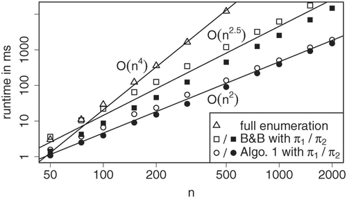Therefore, Algorithm 1 only takes $\mathcal{O}\left(n^{\frac{m-1}{2}}\right)$ operations to determine a p-value above the threshold θ. Figure 6 shows runtime as a function of n for m = 5. Whereas the runtime of the full enumeration method depends only on the parameters m and n, the runtime of the implementation of Algorithm 1 described in Section 3.3 depends on both the parameter π and the observation x. As with the branch and bound approach, the uniform null hypothesis results in a longer runtime than sparse null hypotheses, but the difference is less pronounced. Furthermore, the runtime of Algorithm 1 increases if the p-value of x is small, which is further investigated in the simulation study of Section 4.1. As the runtime increases exponentially in m, Algorithm 1 is only feasible if the number of categories m is small.

Fig. 6 Mean runtime across 10 samples with p-values of about 0.001 under null hypotheses ${\pi }_1=(0.2,0.2,0.2,0.2,0.2)$ and ${\pi }_2=(0.01,0.19,0.2,0.3,0.3)$, respectively, using full enumeration, the branch and bound (B&B) approach and Algorithm 1.

Proposition 7.

Let $T\in \{T^{{\chi }^2},T^G,T^{\mathrm{\mathbb{P}}}\},\alpha \in (0,1)$ and $\pi \in {\Delta }_{m-1}$. Then there exists $c=c(\alpha ,\pi )$ such that $A_{n,\pi }^T(\alpha )\subset B_{\sqrt{n}c}(n\pi )$ for sufficiently large n.

Proof.

Consider the canonical extension $\overline{T}$ of T to ${\overline{\Omega }}_{m,n}=\{x\in {ℝ}_{\ge 0}^m|x_1+\cdots +x_m=n\}$ and let ${\overline{B}}_{n,r}(y)=\{x\in {\overline{\Omega }}_{m,n}|d(x,y)\le r\}$ denote a ball in ${\overline{\Omega }}_{m,n}$ with boundary $\partial {\overline{B}}_{n,r}(y)=\{x\in {\overline{\Omega }}_{m,n}|d(x,y)=r\}$. Let $r_0={\min }_j{\pi }_j>0$ and $n_0\in \mathbb{N}$. If $n\ge n_0$, then every $x\in \partial {\overline{B}}_{n,\sqrt{n{n}_0}{r}_0}(n\pi )$ can be written as $x=x(n,x_0):=n\pi +\sqrt{n{n}_0}(x_0-\pi )$ for some $x_0\in \partial {\overline{B}}_{1,r_0}(\pi )$.

Let $t_{n,1-\alpha }=\min \{t\in ℝ|{\mathrm{\mathbb{P}}}_{\pi }(T_n\le t)\ge 1-\alpha \}$ be the $(1-\alpha )$-quantile of $T_n=T(X_n),X_n\sim {\mathcal{M}}_m(n,\pi )$ for $n\in \mathbb{N}$. As T_n converges to ${\chi }_{m-1}^2$ in distribution, the sequence $(t_{n,1-\alpha })$ of quantiles converges to the $(1-\alpha )$-quantile ${\chi }_{m-1,1-\alpha }^2$ (see, Van der Vaart 1998, Lemma 21.2). Consequently, the maximum $t={\max }_n{t}_{n,1-\alpha }$ exists, and the set $A_n=\{x\in {\overline{\Omega }}_{m,n}|\overline{T}(x)\le t\}$ contains the acceptance region $A_{n,\pi }^T(\alpha )$ for every n.

As $\overline{T}$ is convex (by Lemma 9 in Appendix C, supplementary materials) and thus has convex sublevel sets, it suffices to show that n₀ can be chosen such that $\min \{\overline{T}(x)|x\in \partial {\overline{B}}_{n,\sqrt{n{n}_0}{r}_0}(n\pi )\}$ converges to a value greater t to ensure that $A_{n,\pi }^T(\alpha )\subset A_n\subset {\overline{B}}_{n,\sqrt{n}\left(\sqrt{n_0}{r}_0\right)}(n\pi )$ for sufficiently large n.

In case $T=T^{{\chi }^2}$, observe that$$\overline{T}(x(n,x_0))=\sum _j\frac{{(x_j(n,x_0)-n{\pi }_j)}^2}{n{\pi }_j}=\sum _j\frac{n_0{(x_{0,j}-{\pi }_j)}^2}{{\pi }_j}$$does not depend on n, and so the canonical extension $\overline{T}$ of the Chi-square statistic at radius $\sqrt{n{n}_0}{r}_0$ is bounded from below by $b(n_0)=\min \{\overline{T}(x)|x\in \partial {\overline{B}}_{n_0,r_0}(n_0\pi )\}$. This bound becomes arbitrarily large as n₀ is increased.

In case $T=T^G$ or $T=T^{\mathrm{\mathbb{P}}}$, if n₀ is fixed, $\overline{T}(x(n,x_0))$ converges uniformly to ${\overline{T}}^{{\chi }^2}(x(n,x_0))$ for $x_0\in \partial {\overline{B}}_{1,r_0}(\pi )$ (by Lemma 10 in Appendix C, supplementary materials). Hence, $\min \{\overline{T}(x)|x\in \partial {\overline{B}}_{n,\sqrt{n{n}_0}{r}_0}(n\pi )\}$ converges to $b(n_0)$. □

4 Application

In this section, the use of the new method is illustrated in a simulation study. On the one hand, this serves to show the improvements in runtime in comparison to some other methods. On the other hand, this sheds some light on the fit of the asymptotic approximation to the probability mass test provided by Theorem 1 for a moderate sample size (n = 100). As a practical application in forecast evaluation, the usage of exact multinomial tests to increase the information conveyed by the calibration simplex (Wilks 2013), a graphical tool used to assess ternary probability forecasts, is outlined.

4.1 Simulation Study

For the simulation study, pairs $({\pi }^{(1)},x^{(1)}),\dots ,({\pi }^{(N)},x^{(N)})$ of null hypothesis parameters and samples were generated as iid realizations of the random quantity (P, X) with $P\sim \mathcal{U}({\Delta }_{m-1})$ being uniformly distributed on the unit simplex and $X|P\sim {\mathcal{M}}_m(n,P)$. For each pair, p-values were computed using various test statistics and algorithms. Thereby, no specific null hypothesis had to be chosen and instead a wide variety was considered. By drawing samples from the null hypotheses, p-values follow a uniform distribution on $[0,1]$. Various aspects of the tests and algorithms in question can be examined using the resulting rich dataset and subsets thereof.

The following results were obtained using $N={10}^6$ such pairs with samples of size n = 100 drawn from multinomial distributions with m = 5 categories. Exact p-values were computed using the implementation of Algorithm 1 provided by the accompanying R package. To illustrate the speedup achieved by the new method in this study, the full enumeration method provided by the xmulti function of the XNomial package (Engels 2015) and the branch and bound approach (Bejerano, Friedman, and Tishby 2004) were applied to the first 10⁴ pairs. Essentially, the computational cost of the full enumeration is constant, independent of the null hypothesis at hand and the resulting p-value, whereas the cost of Algorithm 1 increases as the p-value decreases and also varies with the null hypothesis similar to the cost of the branch and bound approach.

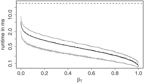
The implementation of Algorithm 1 took an average of 0.59 ms to compute a p-value, improving on the branch and bound approach (1.78 ms), even though the latter only computes p-values for the log-likelihood ratio test, and full enumeration (29.76 ms). Perhaps surprisingly, Monte Carlo estimation (using xmonte from XNomial, which simulates 10,000 samples by default) took almost twice as long (53.49 ms) as the full enumeration. Figure 7 illustrates the connection between runtime and size of the resulting p-values for the new method. As there are other factors influencing the runtime and the implementation computes p-values for multiple statistics simultaneously, samples were ordered by their mean p-value ${\overline{p}}_T=\frac{1}{3}(p_{T^{\mathrm{\mathbb{P}}}}+p_{T^{{\chi }^2}}+p_{T^G})$ and put in groups of 1000 samples with similar mean p-value (in particular, the groups contain samples with p-values in between the empirical $\left(\frac{a}{1000}\right)$- and $\left(\frac{a+1}{1000}\right)$-quantile for $a=0,\dots ,999$). The figure shows mean runtime in each group as well as the 5%- and 95%-quantile.

Fig. 7 Runtime against mean p-value in groups of 1000 samples with similar mean p-value. The black line shows mean runtime per group, whereas the gray lines are the 5% and 95%-quantile. The dashed line shows the mean runtime using full enumeration.

To illustrate the fit of the classical Chi-square approximation, the probability of a Chi-square distribution with m – 1 degrees of freedom exceeding the values of the test statistics for each pair were computed. Figure 8 shows relative errors of the asymptotic approximations to the p-values for the three test statistics. Given a test statistic T and asymptotic approximation ${\tilde{p}}_T={\tilde{p}}_T(x,\pi )$ to the exact p-value $p_T=p_T(x,\pi )$, the relative error is the deviation from the exact value in parts of said value, $\frac{{\tilde{p}}_T-p_T}{p_T}$. The asymptotic approximation to the Chi-square statistic is quite accurate in most cases, but tends to underestimate small p-values (< 0.1). The asymptotic approximation to the log-likelihood ratio statistic tends to slightly underestimate p-values on average. 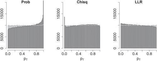While the exact p-values are valid in that ${\mathrm{\mathbb{P}}}_{\pi }(p_T(X,\pi )\le \alpha )\le \alpha$ for all $\alpha \in [0,1]$, underestimation may result in invalid p-values. Asymptotic approximations of Pearson’s Chi-square and the log-likelihood ratio have been studied well, and the classical Chi-square approximations can be improved by using moment corrections (see Cressie and Read 1989, and references therein). Furthermore, the errors typically increase if some category has small expectation under the null hypothesis. The approximation to the probability mass p-values provided by Theorem 1 produces somewhat larger errors especially for large p-values, and it clearly overestimates the p-values. This is emphasized by the fact that within the simulation data only a vanishingly small number of p-values was slightly underestimated, all of which were well over 0.9. Figure 9 illustrates how estimation errors influence the distribution of the resulting p-values. Whereas the exact p-values appear to follow a uniform distribution, the asymptotic p-values clearly deviate from uniformity. For the probability mass statistic, the asymptotic test yields a conservative test, whereas the asymptotic log-likelihood ratio test (and also the asymptotic Chi-square test at small significance levels) is slightly anti-conservative.

Fig. 8 Relative errors of asymptotic approximations to p-values for probability mass (Prob), Chi-square (Chisq) and log-likelihood ratio (LLR) test statistic. The plots were obtained using the same grouping scheme as in Figure 7.

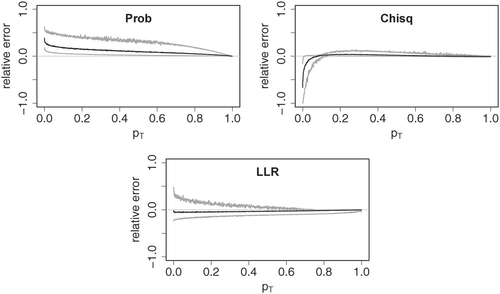
Fig. 9 Histograms of asymptotic approximations to p-values for probability mass (Prob), Chi-square (Chisq), and log-likelihood ratio (LLR) test statistic in black. The gray histograms show respective exact p-values. The rightmost bar within the left histogram is not fully shown and extends further up to over 30000 counts.

Figure 10 shows relative differences between exact p-values obtained with the three test statistics. Given test statistics T and $T\prime$, the relative difference between p-values $p_T=p_T(x,\pi )$ and $p_{T\prime }=p_T(x,\pi )$ is $\frac{p_T-p_{T\prime }}{{\overline{p}}_T}$, where ${\overline{p}}_T=\frac{p_T+p_{T\prime }}{2}$. It can be seen that the choice of test statistic can make quite a difference. A closer look at the simulation data revealed that these differences tend to be smaller if expectations for all categories are large under the null. To provide some numerical insights, Table 1 lists exact and asymptotic p-values.

Fig. 10 Relative differences between exact p-values of probability mass (Prob), Chi-square (Chisq), and log-likelihood ratio (LLR) test statistic against mean of compared p-values. The plots were obtained using the same grouping scheme as in Figure 7.

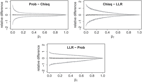
Table 1 Exact p-values p_T and asymptotic p-values ${\tilde{p}}_T$ of five randomly selected pairs $(x,\pi )$ with $0.01<p_{T^G}(x,\pi )<0.1$.

π	$p_{T^{\mathrm{\mathbb{P}}}}$	${\tilde{p}}_{T^{\mathrm{\mathbb{P}}}}$	$p_{T^{{\chi }^2}}$	${\tilde{p}}_{T^{{\chi }^2}}$	$p_{T^G}$	${\tilde{p}}_{T^G}$
$(0.116,0.225,0.259,0.002,0.398)$	0.0068	0.0092	0.0190	0.0073	0.0126	0.0172
$(0.038,0.079,0.224,0.387,0.272)$	0.1150	0.1268	0.1437	0.1469	0.0361	0.0307
$(0.595,0.129,0.093,0.064,0.118)$	0.0447	0.0495	0.0477	0.0482	0.0719	0.0665
$(0.497,0.217,0.223,0.057,0.007)$	0.0761	0.0994	0.0803	0.0741	0.0461	0.0498
$(0.243,0.022,0.237,0.373,0.125)$	0.0474	0.0566	0.0508	0.0507	0.0628	0.0568

4.2 The Calibration Simplex

Turning to an application in forecast verification, consider a random variable X and a probabilistic forecast F for X. For an introduction to probabilistic forecasting in general, see Gneiting and Katzfuss (2014). A probabilistic forecast is said to be calibrated if the conditional distribution of the quantity of interest given a forecast coincides with the forecast distribution, that is,(4) $$X|F\sim F$$(4) holds almost surely. Suppose now that X maps to one of three distinct outcomes only. Then, a probabilistic forecast is fully described by the probabilities it assigns to each outcome. In this case, the calibration simplex (Wilks 2013) can be used to graphically identify discrepancies between predicted probabilities and conditional outcome frequencies. Given iid realizations $(f_1,x_1),\dots ,(f_N,x_N)$ consisting of forecast probabilities (vectors within the unit 2-simplex) and observed outcomes encoded 1, 2, and 3, forecast-outcome pairs with similar forecast probabilities are grouped according to a tessellation of the probability simplex. Thereafter, calibration is assessed by comparing average forecast and actual outcome frequencies within each group.

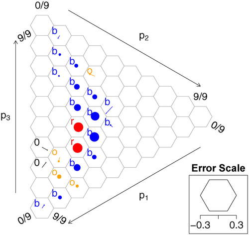
As illustrated in Figure 11, the calibration simplex is a graphical tool used to conduct this comparison visually. The groups are determined by overlaying the probability simplex with a hexagonal grid. The circular dots correspond to nonempty groups of forecasts given by a hexagon. The dots’ areas are proportional to the number of forecasts per group. A dot is shifted away from the center of the respective hexagon by a scaled version of the difference in average forecast probabilities and outcome frequencies. This provides valuable insight into the forecast’s distribution and the conditional distribution of the quantity of interest. However, it is not apparent how big the differences may be merely by chance.

Fig. 11 Calibration Simplex with color-coded p-values from the log-likelihood ratio statistic evaluating a total of 21,240 club soccer predictions by FiveThirtyEight (https://projects.fivethirtyeight.com/soccer-predictions/) for matches from September 2016 until April 2019. Outcomes are encoded as $1=$ “home win”, $2=$ “draw” and $3=$ “away win”. Only groups containing at least 10 forecasts are shown. Blue (b) indicates a p-value $p_{T^G}$ > 0.1, orange (o) $0.1>p_{T^G}\ge 0.01$, red (r) $p_{T^G}<0.01$ and black (0) $p_{T^G}=0$.

If the forecast is calibrated, then, by (4), the outcome frequencies $\overline{x}$ within a group of size n with mean forecast $\overline{f}$ follow a generalized multinomial distribution (the multinomial analog of the Poisson binomial distribution), that is, a convolution of multinomial distributions $\mathcal{M}(1,f_i)$ with parameters $f_1,\dots ,f_n\in {\Delta }_{m-1}$. If these parameters only deviate little from their mean $\overline{f}=\frac{1}{n}\sum _i{f}_i$, then, presumably, the generalized multinomial distribution should not deviate much from a multinomial distribution with parameter $\overline{f}$. Under this presumption, multinomial tests can be applied to quantify the discrepancy within each group through a p-value. As the number of outcomes m = 3 is small, exact p-values are efficiently computed by Algorithm 1 even for large sample sizes n.

In Figure 11, p-values obtained from the log-likelihood ratio statistic are conveyed through a coloring scheme. Note that a p-value is exactly zero only if an outcome is forecast to have zero probability and said outcome still realizes. Figure 11 was generated using the R package CalSim (Resin 2021).

The calibration simplex can be seen as a generalization of the popular reliability diagram. In light of this analogy, the use of multinomial tests to assess the statistical significance of differences in predicted probabilities and observed outcome frequencies serves the same purpose as consistency bars in reliability diagrams introduced by Bröcker and Smith (2007). Consistency bars are constructed using Monte Carlo simulation. To justify the above presumption, the multinomial p-values used to construct Figure 11 were compared to p-values computed from 10,000 Monte Carlo samples obtained from the generalized multinomial distributions. To this end, the standard deviation of the Monte Carlo p-values was estimated using the estimated p-value in place of the true generalized multinomial p-value. Most of the multinomial p-values were quite close to the Monte Carlo estimates with an absolute difference less than two standard deviations, whereas two of them deviated on the order of 6 to 8 standard deviations from the Monte Carlo estimates, which nonetheless resulted in a relatively small absolute error. In particular, using the Monte Carlo estimated p-values did not change Figure 11. As computation of the Monte Carlo estimates from the generalized multinomial distributions is computationally expensive, the multinomial p-values serve as a fast and adequate alternative. Further improving uncertainty quantification within the calibration simplex is a subject for future work.

5 Concluding Remarks

A new method for computing exact p-values was investigated. It has been illustrated that the new method works well when the number m of categories is small. This results in a concrete speedup in practical applications as illustrated through a simulation study. As a further application not discussed in this work, the new method appears to be well suited to determine level set confidence regions discussed in Chafai and Concordet (2009) and Malloy, Tripathy, and Nowak (2021). When m is too large for exact methods to be feasible, other methods may be used to approximate exact p-values as hinted at in Appendix D, supplementary materials. Such an approach may be added to the ExactMultinom package in a future version.

Regarding the choice of test statistic, the “exact multinomial test” was treated as a test statistic and the asymptotic distribution of the resulting probability mass statistic was derived. Like most prominent test statistics, the probability mass statistic yields unbiased tests for the uniform null hypothesis. It was shown that a randomized test based on the probability mass statistic can be characterized in that it minimizes the respective (weighted) acceptance region.

Although asymptotic approximations work well in many use cases, there are cases, where these approximations are not adequate, for example, when dealing with small sample sizes or small expectations. On the other hand, there is nothing to be said against the use of exact tests whenever feasible, and it is recommended in the applied literature (McDonald 2009, p. 83) for samples of moderate size up to 1000. As the available implementations of exact multinomial tests in R use full enumeration, the new implementation increases the scope of exact multinomial tests for practitioners.

Acknowledgments

The author would like to thank Tilmann Gneiting, Alexander I. Jordan, and Sebastian Lerch for helpful comments, discussions and continued encouragement as well as two anonymous reviewers for their constructive comments.

Supplementary Materials

Appendices:Mathematical details complementing the proofs of Theorem 1, Proposition 4, and Proposition 7, and a short discussion of other methods. (pdf)

Package ExactMultinom: R package containing the implementation described in Section 3. (GNU zipped tar file)

Additional code: R code used for the simulation study in Section 4. (.R file)

Disclosure Statement

The author reports there are no competing interests to declare.

Additional information

Funding

This work has been supported by the Klaus Tschira Foundation.

Notes

1 Randomized tests like this traditionally arise in the theory of uniformly most powerful tests, see for example, Lehmann and Romano (2005, chap. 3).

References

- Baglivo, J., Olivier, D., and Pagano, M. (1992), “Methods for Exact Goodness-of-Fit Tests,” Journal of the American Statistical Association, 87, 464–469. DOI: 10.1080/01621459.1992.10475227.
- Beals, R., and Wong, R. (2010), Special Functions: A Graduate Text (Vol. 126), Cambridge: Cambridge University Press.
- Bejerano, G. (2006), “Branch and Bound Computation of Exact p-values,” Bioinformatics, 22, 2158–2159. DOI: 10.1093/bioinformatics/btl357.
- Bejerano, G., Friedman, N., and Tishby, N. (2004), “Efficient Exact p-value Computation for Small Sample, Sparse, and Surprising Categorical Data,” Journal of Computational Biology, 11, 867–886. DOI: 10.1089/cmb.2004.11.867.
- Bröcker, J., and Smith, L. A. (2007), “Increasing the Reliability of Reliability Diagrams,” Weather and Forecasting, 22, 651–661. DOI: 10.1175/WAF993.1.
- Chafai, D., and Concordet, D. (2009), “Confidence Regions for the Multinomial Parameter with Small Sample Size,” Journal of the American Statistical Association, 104, 1071–1079. DOI: 10.1198/jasa.2009.tm08152.
- Cohen, A., and Sackrowitz, H. B. (1975), “Unbiasedness of the Chi-square, Likelihood Ratio, and other Goodness of Fit Tests for the Equal Cell Case,” The Annals of Statistics, 3, 959–964. DOI: 10.1214/aos/1176343197.
- Cressie, N., and Read, T. R. C. (1984), “Multinomial Goodness-of-Fit Tests,” Journal of the Royal Statistical Society, Series B, 46, 440–464. DOI: 10.1111/j.2517-6161.1984.tb01318.x.
- Cressie, N., and Read, T. R. C. (1989), “Pearson’s X2 and the Loglikelihood Ratio Statistic G2: A Comparative Review,” International Statistical Review, 57, 19–43. DOI: 10.2307/1403582.
- Engels, B. (2015), XNomial: Exact Goodness-of-Fit Test for Multinomial Data with Fixed Probabilities. R package version 1.0.4. Available at https://CRAN.R-project.org/package=XNomial.
- Gibbons, J. D., and Pratt, J. W. (1975), “P-values: Interpretation and Methodology,” The American Statistician, 29, 20–25.
- Gneiting, T., and Katzfuss, M. (2014), “Probabilistic Forecasting,” Annual Review of Statistics and its Application, 1, 125–151. DOI: 10.1146/annurev-statistics-062713-085831.
- Hirji, K. F. (1997), “A Comparison of Algorithms for Exact Goodness-of-Fit Tests for Multinomial Data,” Communications in Statistics - Simulation and Computation, 26, 1197–1227. DOI: 10.1080/03610919708813435.
- Keich, U., and Nagarajan, N. (2006), “A Fast and Numerically Robust Method for Exact Multinomial Goodness-of-Fit Test,” Journal of Computational and Graphical Statistics, 15, 779–802. DOI: 10.1198/106186006X159377.
- Koehler, K. J., and Larntz, K. (1980), “An Empirical Investigation of Goodness-of-Fit Statistics for Sparse Multinomials,” Journal of the American Statistical Association, 75, 336–344. DOI: 10.1080/01621459.1980.10477473.
- Kotze, T. J. V. W., and Gokhale, D. V. (1980), “A Comparison of the Pearson-X2 and Log-Likelihood-Ratio Statistics for Small Samples by Means of Probability Ordering,” Journal of Statistical Computation and Simulation, 12, 1–13. DOI: 10.1080/00949658008810422.
- Lehmann, E. L., and Romano, J. P. (2005), Testing Statistical Hypotheses. Springer Texts in Statistics (3rd ed.), New York: Springer.
- Malloy, M. L., Tripathy, A., and Nowak, R. D. (2021), “Optimal Confidence Sets for the Multinomial Parameter,” in 2021 IEEE International Symposium on Information Theory (ISIT), pp. 2173–2178. DOI: 10.1109/ISIT45174.2021.9517964.
- McDonald, J. H. (2009), Handbook of Biological Statistics (2nd ed.), Baltimore: Sparky House Publishing.
- Menzel, U. (2013), EMT: Exact Multinomial Test: Goodness-of-Fit Test for Discrete Multivariate Data. R package version 1.1. Available at https://CRAN.R-project.org/package=EMT.
- Murota, K. (2003), Discrete Convex Analysis. SIAM Monographs on Discrete Mathematics and Applications, Philadelphia: Society for Industrial and Applied Mathematics (SIAM).
- Pérez, T., and Pardo, J. A. (2003), “On Choosing a Goodness-of-Fit Test for Discrete Multivariate Data,” Kybernetes, 32, 1405–1424. DOI: 10.1108/03684920310493323.
- R Core Team (2020), R: A Language and Environment for Statistical Computing, Vienna, Austria: R Foundation for Statistical Computing. Available at https://www.R-project.org/.
- Radlow, R., and Alf, E. F. J. (1975), “An Alternate Multinomial Assessment of the Accuracy of the χ2 Test of Goodness of Fit,” Journal of the American Statistical Association, 70, 811–813.
- Rahmann, S. (2003), “Dynamic Programming Algorithms for Two Statistical Problems in Computational Biology,” in Algorithms in Bioinformatics. WABI 2003., Lecture Notes in Computer Science (Vol. 2812), pp. 151–164, Berlin, Heidelberg: Springer.
- Resin, J. (2020), ExactMultinom: Multinomial Goodness-of-Fit Tests. R package version 0.1.2. Available at https://CRAN.R-project.org/package=ExactMultinom.
- Resin, J. (2021), CalSim: The Calibration Simplex. R package version 0.5.2. Available at https://CRAN.R-project.org/package=CalSim.
- Tate, M. W., and Hyer, L. A. (1973), “Inaccuracy of the X2 Test of Goodness of Fit when Expected Frequencies are Small,” Journal of the American Statistical Association, 68, 836–841.
- Van der Vaart, A. W. (1998), Asymptotic Statistics, Volume 3 of Cambridge Series in Statistical and Probabilistic Mathematics, Cambridge: Cambridge University Press.
- Wakimoto, K., Odaka, Y., and Kang, L. (1987), “Testing the Goodness of Fit of the Multinomial Distribution based on Graphical Representation,” Computational Statistics & Data Analysis, 5, 137–147.
- West, E. N., and Kempthorne, O. (1972), “A Comparison of the Chi2 and Likelihood Ratio Tests for Composite Alternatives,” Journal of Statistical Computation and Simulation, 1, 1–33. DOI: 10.1080/00949657208810001.
- Wilks, D. S. (2013), “The Calibration Simplex: A Generalization of the Reliability Diagram for Three-Category Probability Forecasts,” Weather and Forecasting, 28, 1210–1218. DOI: 10.1175/WAF-D-13-00027.1.