Selection of optimal validation methods for quantitative structure–activity relationships and applicability domain

ABSTRACT

This brief literature survey groups the (numerical) validation methods and emphasizes the contradictions and confusion considering bias, variance and predictive performance. A multicriteria decision-making analysis has been made using the sum of absolute ranking differences (SRD), illustrated with five case studies (seven examples). SRD was applied to compare external and cross-validation techniques, indicators of predictive performance, and to select optimal methods to determine the applicability domain (AD). The ordering of model validation methods was in accordance with the sayings of original authors, but they are contradictory within each other, suggesting that any variant of cross-validation can be superior or inferior to other variants depending on the algorithm, data structure and circumstances applied. A simple fivefold cross-validation proved to be superior to the Bayesian Information Criterion in the vast majority of situations. It is simply not sufficient to test a numerical validation method in one situation only, even if it is a well defined one. SRD as a preferable multicriteria decision-making algorithm is suitable for tailoring the techniques for validation, and for the optimal determination of the applicability domain according to the dataset in question.

KEYWORDS:

• Cross-validation
• resampling
• comparison of methods
• ranking
• applicability domain
• multicriteria decision-making

Introduction

The debate about whether cross-validation [1–3] or external validation [4,5] is better (superior, compulsory) seems to have come to a standstill around the mid-2010s [6,7].

An empirical meta-analysis [8] compared the performance of internal cross- versus external validation for 28 studies on molecular classifiers and concluded that cross-validation variants overestimate classifier performance in the majority of cases. Therefore, they suggest routine external validation of molecular classifiers [8].

In contrast, Chatterjee and Roy [9] have recently suggested avoiding overestimation of performance of 2D-QSAR models, by using cross-validation strategies.

A single split external test cannot be considered ground truth. On the contrary, single split and external validation are different [4]. The Gütlein-Gramatica debate was settled with Gramatica suggesting multiple external testing: ‘To avoid the limitation of using only a single external set, we, in our recent papers [10] always verify our models on two/three different prediction sets’ [11].

Some sources about performance merits are summarized next: the square of multiple correlation coefficients for the test set can be defined differently (i.e. the explained variance for the prediction model, generally denoted by Q²) [12]. Concordance correlation coefficient (CCC) is recommended as a measure of real external predictivity [13]. On the other hand, a detailed study [14] on mapping between the CCC and the mean squared error showed that CCC is overoptimistic, and the authors advised against the replacement of traditional L_p-norm loss functions by CCC-inspired loss functions in multivariate regressions. Shayanfar and Shayanfar have recently disclosed that the ranges for performance parameters defining good, moderately good and bad models are contradictory and no advocated way exists, which shows superiority from all points of view (according to all performance parameters) [15]. Significance thresholds for performance parameters are strongly application-dependent [16].

Several sources reveal some problems of k-fold cross-validation [16–18]. A simple permutation of rows may lead to contradictory conclusions about the significance of the models [16]. Rakhimbekova et al. find that k-fold cross-validation is overoptimistic, i.e. it provides biased predictions for the modelling of chemical reactions [17]. A comparison of validation variants revealed that the conclusions can vary according to the data structure; row randomization is suggested as the first step of data analysis [18].

As early as in 2007, Rücker et al. called attention to the fact that a randomization (permutation) test can be performed differently, not only by y-scrambling [19]; yet his recommendations are rarely followed, if at all.

There are many variants of cross-validation (CV): leave-one-out, leave-many-out, bootstrap, bootstrapped Latin partition, Kennard-Stone algorithm, etc., with realizations of i) row-wise, pattern-wise (Wold), etc. [20]; ii) Venetian blinds, contiguous block, etc. [21]. Reliable estimation of prediction errors for QSAR models can be completed by using double cross-validation [22,23], also in a repeated form [22]. The variants should also be disclosed to obtain reproducible results.

A bunch of mostly new, individual statements are gathered below to illustrate the complexity of the validation aspects.

How to split training, validation (calibration) and test set is of crucial importance [3,24]. In a detailed classification modelling, Xu and Goodacre have ended up with statements as i) a good balance between training and test set is a prerequisite to obtain a stable estimation of model performance, and ii) there are no superior methods/parameter combinations, which would always give significantly better results than others, i.e. which method is to be used for data splitting (and with which parameters) cannot be defined a priori [24]. A recursive variable elimination algorithm was elaborated using repeated double cross-validation. The robust algorithm improves the predictive performance and minimizes the probability of overfitting and false-positive rates at the same time [25]. Cross-validation (single split) and even a double cross-validation ‘provide little, if any, additional information’ to evaluate regression models [26]. Guo and his colleagues [27] uncovered two types of common mistakes of cross-validation in Raman spectroscopy: i) splitting the dataset into training and validation datasets improperly; ii) applying dimension reduction in the wrong position of the cross-validation loop. Several combinations of different cross-validation variants (c.f., ref. [21]) and model-building techniques were used to reveal their complexity. The gap between the squared multiple correlation coefficients for calibration (r²) and for the test set (Q²) has changed in a systematic manner according to the algorithms applied [28]. As multiple linear regression can be taken as a kind of standard, Kovács et al. have investigated the sample size dependence of validation parameters [29].

The fast development of the big data and machine learning fields requires novel validation techniques. Here, two examples are indicated only: Novel validation options (convergent and divergent ones) have been developed for machine learning models (convergent means one dataset and many classifiers—also called consensus modelling—whereas divergent means more external datasets). Suggestions have been made on i) how to acquire valid external data, ii) how to determine the number of times an external validation needs to be performed and iii) what to do when multiple external validations disagree with each other [30]. Coefficient of determination (r-squared) is more informative and truthful than symmetric mean absolute percentage error (SMAPE). Moreover, r² does not have the interpretability limitations contrary to error variants (mean absolute error) [31].

Hence, it is somewhat odd, annoying and astonishing (!) that older, refuted and outdated sources are still cited, but at the same time, new examinations also produce contradictory conclusions. The well recognized international standards [32,33] are not always followed. Cross-validation is not one, but a set of algorithms, which need to be applied differently in different contexts. The same is true for external validation, as well. Herewith it is not feasible to put the jungle of contradictory references in order, but some reasons are enumerated here.

The reasons are manyfold: i) the validation practices are different for various scientific disciplines; ii) the aim of validation can be different (model optimization, feature selection, understanding the data structure, etc.); iii) the modelling methods are diverse (regression, classification); iv) the peculiarities (idiosyncrasies) of datasets are different; v) the types and number of performance parameters provide conflicting results, and many others.

A simple and trivial conclusion would be that the recommended validation techniques are dataset dependent and should be carried out independently again and again, from case to case.

However, the question remains: why are there so many independent studies with contradictory conclusions? What kind of validation variant should be selected for a new examination, if the data structure has not been known yet?

Hence, the primary aim of this study is to compare (numerical) validation methods (bounded to selection criteria) in a fair way. If the performance criterion concerns an ‘on-line modelling and prediction’ situation, the model comparison includes this case, as well. Ranking (ordering and, if possible, grouping) of the performance criteria is also the goal of the present study, definitely. To date, numerous methods are known to determine the applicability domain, but their validation is scarcely studied and recommendations are hard to find.

A feasible assumption is that all types of validation approximate the true performance with a certain level of error. Similarly, the performance parameters are not error-free quantities. Even worse, they can produce contradictory model rankings (feature selection, etc.). Fortunately, well-known algorithms were elaborated in the field of Multi Criteria Decision Analysis (MCDA), also termed as Post-Pareto-analysis or multiobject optimization.

‘MultiCriteria Decision-Making (MCDM) strategies are used to rank various alternatives (scenarios, samples, objects, etc.) on the basis of multiple criteria, and are also used to make an optimal choice among these alternatives. In fact, the assessment of priorities is the typical premise before a final decision is taken’ [34]. The highly degrading characteristic of the total ranking methods is the subjectivism: i) the choice of a performance index is subjective, ii) the selection and definition of attribute weights are subjective and iii) the choice of preference functions is also subjective [34]. The author is well aware of the fact that some authors [35] claim to define objective weights. However, the selection of mathematical procedures to calculate them remains subjective.

Therefore, a fair method comparison algorithm was applied: sum of ranking differences (SRD) as a method of ranking and grouping [36]. Several, carefully selected case studies are employed, and fair evaluations are expected without influencing the results with the beliefs of the original authors. This work explains the existence of contradictory conclusions in the literature and suggests solutions to overcome the difficulties of model validation.

Calculation method

Since its invention in 2010 [36], sum of ranking differences achieved a considerable record: As of May 16 2023, Scopus lists 559 research papers by the keyword ‘sum of ranking differences’ (search within all fields). SRD is entirely general, and it has been applied for column selection in chromatography [36,37], for comparison of compounds based on their ADMET characteristics [38], for outlier detection (without tuning parameter selections) [39], for lipophilicity assessment [40–42], for ranking academic excellence [43], to develop novel similarity indices [44,45], to tea grade quantification [46], just to name a few.

The utilization of SRD has proliferated as it turned out to be one of the best MCDA techniques [3,47]. Eight MCDM algorithms were compared, and their consensus was realized by the sum of ranking differences without using subjective weights [47].

The validation methods are to be arranged in a matrix form: objects are placed in the rows, whereas variables (validation methods or selection criteria) to be compared are arranged in the columns. Ranking should be carried out for each validation method. If the ‘governing’ (reference) ranking is known, it should be compared with the rankings for each individual ranking produced by the variables (validation methods) one by one. Then, absolute values for differences between the reference ranking and individual ones are calculated and summarized for each validation method. The absolute values of differences for the ‘governor’ (benchmark) and individual rankings are summed up. The procedure is repeated for each individual validation method (or criterion), therefore one SRD value will be assigned to each method (or criteria). The SRD values obtained in such a way order (rank and group) the methods simply. The reference ranking—if not known a priori—can be different: for analysing residuals and error rates, the row-wise minimum is the best choice, whereas for correct classification rates the row-wise maximum is the best one. In other cases, the average might be chosen as a suitable benchmark (or median, if the distribution is skewed). The rationale behind is that we are better off using the average than any other individual reference scale, even if the average (median) is biased and/or highly variable. Consensus modelling (ensemble averaging) is one of the success stories in the modelling field (rational drug design, QSAR, etc.). The theoretical foundation is given in the book of Hastie et al. on the example of smoothing and assuming additive Gaussian noise: ‘ … the bootstrap … allows us to compute maximum likelihood estimates in settings where no formulas are available’ [48].

We can always define a hypothetical model (method), which produces average values. We may be interested in knowing which models, methods, etc., are the most similar and/or dissimilar to the hypothetical one, and how the models are grouped regarding the average as reference. SRD corresponds to the principle of parsimony and provides an easy tool to evaluate the validation methods: the smaller the sum, the better the method, because the smaller discrepancies are preferred as compared to the reference.

As all variants of cross-validation and all criteria were determined on the same scale (0 < r², Q² < 100; 0 < No. of PC < Nmax; 0 < classification rate < 100), no data preprocessing was necessary.

If the number of rows (objects) is different, the SRD values cannot be compared directly. To make the different case studies comparable, the resulting SRD values were scaled between 0 and 100 (which is possible due to the existence of an exact upper limit for the SRD values for any given number of objects, which can be easily determined).

The SRD procedure contains a kind of validation called CRRN (comparison of ranks by random numbers) [49]. A recursive algorithm calculates the discrete distribution for a small number of objects (n< 14). The discrete (true) distribution of simulated (random) SRD-s is approximated with a normal distribution for any number of objects larger than 13.

The reliability (significance) of ranking by SRD can be checked easily. The distance between true SRD values and SRD values by chance shows the reliability. The significance can be tested by nonparametric tests such as the Wilcoxon matched pair test. If the SRD values derived from random numbers are in the same range as the true SRD values, the models built on real data are indistinguishable from random ranking, even if physical significance can be assigned to the parameters of the model.

Results

Case study no. 1. Comparison of validation variants

As outlined in the introduction, reputable scientists cannot agree on the performance of cross- and external validations. Herewith, the results of two scientific schools are compared: that of Gramatica’s [5] and that of Hawkins’ [50].

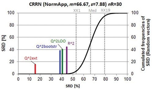
Gramatica has given the statistical performance parameters for 30 linear models containing two descriptors each. The models predicted mutagenicity of 48 nitro substituted polycyclic aromatic hydrocarbons (39 compounds were selected in the training set and 17 compounds in the prediction set). The following performance indicators were calculated: square of multiple correlation coefficient for the training set (R^2), leave-one-out cross-validated correlation coefficient (Q^2LOO), bootstrap cross-validated correlation coefficient (Q^2bootstr) and correlation coefficient calculated on the external test set (Q^2ext). Performance parameters are from Table 1 in ref. [5].

Table 1. Correlation matrix of performance indicators from Table 1 in ref. [50]. Significant correlations are indicated by bold (at the 5% level, comparing to ρ = 0). The notations are indicated in the text.

	Q^2 U	Q^2 Uext	Q^2Sn1	Q^2Sn2	Q^2S	Q^2Sext	Q^2Gn1	Q^2Gn2	Q^2G	Q^2Gext	Q^2E	Q^2Eext
Q^2 U	1.000	−0.797	0.590	0.837	0.745	−0.598	0.466	0.604	0.380	−0.666	0.146	−0.570
Q^2 Uext	−0.797	1.000	−0.576	−0.825	−0.676	0.816	−0.457	−0.698	−0.546	0.804	−0.309	0.850
Q^2Sn1	0.590	−0.576	1.000	0.712	0.582	−0.621	0.498	0.742	0.640	−0.475	0.575	−0.442
Q^2Sn2	0.837	−0.825	0.712	1.000	0.719	−0.824	0.433	0.741	0.479	−0.711	0.317	−0.645
Q^2S	0.745	−0.676	0.582	0.719	1.000	−0.604	0.337	0.672	0.508	−0.593	0.572	−0.577
Q^2Sext	−0.598	0.816	−0.621	−0.824	−0.604	1.000	−0.380	−0.752	−0.549	0.643	−0.468	0.811
Q^2Gn1	0.466	−0.457	0.498	0.433	0.337	−0.380	1.000	0.590	0.828	−0.568	0.302	−0.303
Q^2Gn2	0.604	−0.698	0.742	0.741	0.672	−0.752	0.590	1.000	0.719	−0.478	0.559	−0.632
Q^2G	0.380	−0.546	0.640	0.479	0.508	−0.549	0.828	0.719	1.000	−0.591	0.643	−0.434
Q^2Gext	−0.666	0.804	−0.475	−0.711	−0.593	0.643	−0.568	−0.478	−0.591	1.000	−0.263	0.675
Q^2E	0.146	−0.309	0.575	0.317	0.572	−0.468	0.302	0.559	0.643	−0.263	1.000	−0.328
Q^2Eext	−0.570	0.850	−0.442	−0.645	−0.577	0.811	−0.303	−0.632	−0.434	0.675	−0.328	1.000

The 30 models provide a reliable basis for ranking. The row averages of performance parameters were considered as the ‘governing feature’ of ranking. The only assumption is that all performance indicators express predictive features of the models with error (with bias and random error). As some of the indicators are overoptimistic (R^2, Q^2LOO) and others are pessimistic (Q^2bootstr, Q^2ext), we may well hope that not only the random errors cancel each other out but the biases as well.

Figure 1 shows unambiguously that external validation is the best (consensus) choice, the bootstrap validation is far worse, LOO is even worse and the worst validation method is the usage of the correlation coefficient for the training set. Still, the validation by r² (training) is better than the random ranking (5% limit can be found at scaled SRD ~ 54 (XX1)).

Figure 1. Scaled sum of ranking difference (SRD) values between 0 and 100 for performance parameters plotted against themselves (x and left y axes). The solid (black) line is an approximation by cumulated Gauss distribution to the discrete distribution of the simulated random numbers given in relative frequencies, right y axis. (XX1 = first icosaile, 5%, XX19 = last icosaile 95%, med = median).

Before drawing an intermediate conclusion, let us compare various modelling methods and consider the performance parameters given by Hawkins et al. [50]. In their Table 1, performance parameters (cross-validated Q² and hold-out r² values) are gathered for (i) usual ridge regression, RR: true 10-fold CV-Q² (Q^2U) and hold-out r² (Q^2Uext); (ii) Soft threshold descriptor selection then RR: naïve one-deep 10-fold CV-Q² (Q^2Sn1), naïve two-deep 10-fold CV-Q² (Q^2Sn2), true 10-fold CV-Q² (Q^2S) and hold-out r² (Q^2Sext); (iii) Gram–Schmidt descriptor selection then RR: naïve one-deep 10-fold CV-Q² (Q^2Gn1), naïve two-deep 10-fold CV-Q² (Q^2Gn2), true 10-fold CV-Q² (Q^2G) and hold-out R² (Q^2Gext); (iv) elastic net: true 10-fold CV-Q² (Q^2E), and hold-out r² (Q^2Eext).

Twenty randomly drawn splits serve as a reliable basis for SRD ranking. Naturally, the splits should not differ considerably; still, the average of 12 performance parameters runs from 0.468 to 0.522 showing the differences in data structure from segments to segments. Test of means suggests a significant difference: p-limit = 0.0226, assuming normal distribution, two-sided t-test for performance parameters (Table 1 in ref. [50]). These differences help in ranking, but no importance should be attributed to them.

The results are visualized in Figure 2.

Figure 2. Scaled sum of ranking difference (SRD) values between 0 and 100 for performance parameters plotted against themselves (x and left y axes). The solid (black) line is an approximation by cumulated Gauss distribution to the discrete distribution of the simulated random numbers given in relative frequencies, right y axis (for notations see text).

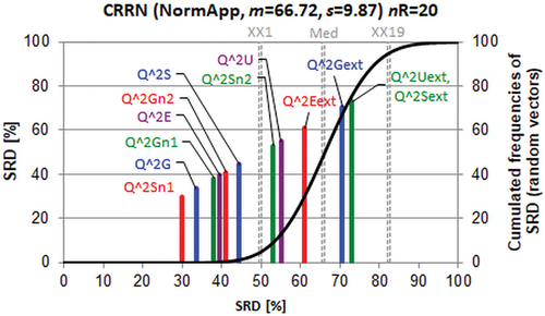
Two groups can be seen immediately; (i) ‘good’ performance indicators (left-hand side) and ‘bad’ ones (right-hand side): Q^2Sn1, Q^2G, Q^2Gn1, Q^2E, Q^2Gn2, Q^2S and Q^2Sn2, Q^2U, Q^2Eext, Q^2Gext, Q^2Uext, Q^2Sext, respectively. All SRD values for the ‘bad’ group are above the 5% error limit (i.e. comparable with random ranking). The close proximity of SRD values suggests that the ordering might vary if other splits or other data were used. The first position of Q^2Sn1 should not be taken seriously, as random splits governed the ranking. However, such proximities as Q^2Gn1 and Q^2E show the closest similarities.

A striking but not surprising conclusion is that external validations are not better than random ranking; all external validation parameters are overlapping with the discrete distribution of random SRD values (approximated by a continuous cumulated Gaussian fit, black line in Figure 1, the fitting parameters are given in the title). It is not surprising because the main message is in accordance with Hawkins et al.’s conclusions [50].

Half of the indicators are commensurable with the random ranking, as expected; the 20 splits were drawn randomly, but the correlation coefficients of the performance criteria vary between –0.825 and +0.850 (Table 1).

Table 1 indicates the significant differences compared to the theoretical ρ = 0. Indeed, Q^2Eext, Q^2Gext, Q^2Uext, Q^2Sext, are positively correlated with each other pairwise and located in the range of random ranking (Figure 2).

Comparing Figures 1 and 2, one can immediately conclude that the ranking procedure (SRD) is perfect; it recapitulates the sayings of the original authors. However, the two conclusions are in full contradiction; in the first case external validation is selected as the best method, whereas in the second case any variants of external validations are ordered in the ‘bad’ group; they, in fact, realize the worst options. Both scientific schools concluded correctly on the basis of the available information. Figure 1 shows the superiority of external validation on the basis of the mutagenicity example of benzene derivatives (48): 30 bivariate models and four types of cross-validation are compared. ‘Some models appear stable and predictive by internal validation parameters (Q^{^}2LOO and Q^2bootstr), but are less predictive (or even unpredictive Q^2ext = 0) when applied to external chemicals’ [5]. On the contrary, the juvenile hormone example (304 compounds), validated by 20 segments, applies different variants of model building, and CV clearly shows that external validation is the worst option (Figure 2).

Case study no. 2. Comparison of statistical tests based on residuals

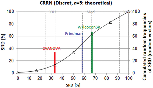
Cederkvist et al. have compared four methods from the point of view of prediction performance [51]. As the statistical tools are applicable in a pair-wise manner only, they compared PLS and PCR models with different numbers of latent variables pairwise in various combinations. Unfortunately, the predicted values or the residuals are not given in their work, i.e. a direct comparison is not possible between SRD ordering and their results. However, Table I in ref. [51] allows a ranking of three statistical tests: CVANOVA, Wilcoxon Signed-Rank test and Friedman test. Five pairs of models served to order the above three tests. Their table contains probability values for testing squared and absolute residuals. The SRD ordering provides exactly the same results for both cases, as expected. The average probabilities were accepted as a reference.

Although the number of pairs is fairly small (5), the finding is in accordance with the original authors’ main conclusion ‘CVANOVA based on the absolute values of the prediction errors seems to be the most suitable method for testing the difference between prediction methods’. The smallest SRD was calculated for CVANOVA (Figure 3). The distorted random distribution (black line connects the points of the discrete distribution) shows that the theoretical SRD distribution is not normal, but still a clear decision can be made. To note, all three methods overlap with the distribution of SRD values for random ranking, but this can be attributed mostly to the small number of objects, which yields an unusually wide SRD distribution.

Figure 3. Scaled sum of ranking difference (SRD) values between 0 and 100 plotted against themselves. The solid (black) line connects the discrete points of theoretical SRD distribution for the simulated random numbers given in relative frequencies, right y axis.

Case study no. 3 Bayesian information criterion or cross-validation?

A recent empirical study questions the usefulness of information criteria (ICs) in selecting the best model. Various ICs (e.g. Akaike’s IC, Bayesian IC, etc.) are used extensively to rank competing models, to select the ‘best-performing’ model(s) from alternatives and to make inferences on variable importance [52]. The authors, as editors, have observed that many submissions … did not evaluate whether the nominal ‘best’ model(s) found using IC is a ‘useful model’ [52].

Toher et al. have compared classification methods in a detailed study [53]. Their intention was to compare classifiers (linear and quadratic discriminant analyses) with variants of partial least squares discriminant analysis (PLS DA, their terminology was ‘regression based’ methods). They applied measured data: 157 honey samples from Ireland (pure and adulterated differently) in various situations (data preprocessing with and without Savitzky-Golay filter, maximum of 10, 20 and 40 PLS components, as well as three different types of training-test splits: (i) correct proportions of pure and each type of adulterant, (ii) correct proportions of pure and adulterated and (iii) unrepresentative proportions of pure and adulterated samples). Different data structures have been considered in various sample sets (Tables 2–5 in ref. [53]) using different kinds of evaluations. Honey samples were drawn from different times. Three batches were adulterated with fructose-glucose mixtures, and one-one batch with fully inverted beet syrup and high fructose corn syrup, each.

Two methods of model selection were compared for each classification variant: fivefold cross-validation (CV) and the Bayesian Information Criterion (BIC). Best classification rates in Tables 2–5 in ref. [53] served as a reliable basis either to compare the variants of regression and model-based discriminant methods, or to compare various tested situations (pure-adulterated, various splits). The ordering by SRD on regression- and on model-based discriminant methods gives interesting and conforms results to the original conclusions (e.g. Savitzky-Golay filtering with a maximum of 10 PLS components is the best, 40 PLS components realize a clear overfit, etc., the results are available from the author upon request). This work aims to compare different situations. As both criteria (BIC and CV) were tested in all situations, also the two criteria can be compared reliably.

Figure 4 shows the frequencies plotted against the scaled sum of ranking differences, unlike the previous figures.

Figure 4. Frequencies of Bayesian information criterion (B) and fivefold cross-validation (C) (y–axis) as a function of scaled sum of ranking differences (x-axis).

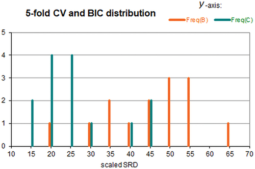
Two distributions can be seen clearly. While there is some overlap, still there is statistical evidence that the two distributions are significantly different. The variances are homogeneous (Levene test, Cochran, Hartley, Bartlett tests all suggest this). Smaller SRD values show the superiority of CV over BIC criterion: scaled-SRD_mean(CV) = 26.4 and scaled-SRD_mean(BIC) = 45.0. The means of SRD values for the two groups are significantly different by t-test (assuming normal distribution); the significance limit is p= 0.000144. Nonparametric tests also confirm significant difference for the two groups: Kolmogorov–Smirnov test (p-limit < 0.01) and Mann–Whitney U-test (p-limit = 0.000674). Naturally, the ranking by SRD can reveal which situations are the best ones and which criteria should (or might) be used in different situations, in case of different data structures. However, it lies outside the scope of present investigations to analyse this in detail.

The above finding is in full accordance with the original authors: ‘ … the vast improvement in classification performance using cross-validation as a model selection method indicates that the penalty term imposed by BIC is not optimum for achieving good classification performance … ’.

The figure clearly shows the problem one should face in model comparison studies. In some cases, BIC and CV are equivalent; in a few cases, BIC is even superior to CV, c.f., Figure 4. However, in the vast majority of cases, the statistical tests suggest that the conclusion is in accordance with the conclusion based on SRD. Hence, it is not sufficient to test a method in one situation only, even if it is a well defined one.

Case study no. 4. Comparison of r² with error terms

Chicco et al. [31] have compared the coefficient of determination (r²) with the symmetric mean absolute percentage error (SMAPE) in several use cases and in two real medical scenarios. They declared that the r² is more informative than SMAPE. Other error measures have interpretability limitations, which include mean square error (MSE), and its rooted variant (RMSE), or the mean absolute error (MAE) and its percentage variant (MAPE).

As SRD incorporates rank transformations, the scaling problem is eliminated. Two tables were united and transposed (Supporting information Tables S1 and S2 of ref. [31]). Average was accepted as the benchmark. Figure 5 visualizes the main message in full accordance with the conclusions of ref. [31].

Figure 5. Comparison of coefficient of determination (r²) and error measures (MAE MSE SMAPE RMSE MAPE, resolving the abbreviations can be found in part 3.3) using the SRD methodology. Notations are the same as in Figures 1–3.

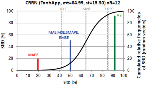
The selection of the reference is mirrored in the SRD plot. As the majority of performance parameters are error measures, the closest ones to the benchmark (SRD = 0) are error-based parameters, as they should be. The best of them is MAPE and all the remaining error measures are indistinguishable from each other and from the random ranking (their line lies between XX1 and XX19). However, SRD is fool proof: the line for r² is located to the right of the 95% probability of random ranking (XX19), i.e. it is the best measure but ranks reversely as compared to error merits. This finding supports the conclusion of the original authors, with an independent multicriteria decision-making tool.

Case study no. 5. Comparison of methods to determine the applicability domain

Standardization always lags behind cutting-edge research. There is no wonder that no validation is included in regulatory documents for defining the applicability domain (AD). Fortunately, the frontier is extending: two attempts could be found to compare validation methods for defining AD [54,55]. The latter one is a special case and concerns QSPR models for chemical reactions only.

Sahigara et al. [54] emphasized that different algorithms for the determination of AD define the interpolation space in several ways, and that the selected thresholds contribute significantly to the extrapolations, while conforming with OECD principles [54]. The analysis of Sahigara et al. was limited to classical AD methodologies used for interpolation space. These classical methodologies can be classified into three groups: i) range-based ii) distance-based and iii) probability density distribution-based methods. Transposes of Tables 6 and 7 of ref. [54] are suitable to compare the AD determination methods in a fair way. The notations are as follows: Euclidean Distance (EUC), City Block (Manhattan) Distance (CBk), Mahalanobis Distance (Mah), k-Nearest neighbour algorithm (k= 5) with Euclidean Distance (5NNEUC), k-Nearest Neighbour algorithm (k= 5) with City Block (Manhattan) Distance (5NNCBk), k-Nearest Neighbour algorithm (k= 5) with Mahalanobis Distance (5NNMah), all distance measures are at p= 95%; Bounding Box (BouB), PCA Bounding Box (PCABouB), Convex Hull (ConvexHull) and Potential Function (PotFunc).

The only highly sensitive decision is the selection of an appropriate gold standard in an SRD analysis. Fortunately, the SRD algorithm allows the usage of a hybrid optimum. As the number of compounds outside the 95% range is on different scales, the median was selected as the best possible choice (outside range, test sets). The squared correlation coefficient of prediction (Q²) was averaged to obtain the optimal benchmark value, whereas minimum was applied to absolute error values (details are given in the Shakigara sheet of the supplementary excel table).

There are some insignificant differences in the middle of the SRD plot (Figure 6); however, the best (Convex Hull) and worst (k-Nearest Neighbour algorithm (k= 5) with Euclidean Distance, 5NNEUCp95) methods to determine the applicability domain can be easily perceived. 5NNEUCp95 is indistinguishable from random ranking, as its line is located right of the XX1 (5%) border. Naturally, the ordering of the methods might change, if other computer codes and performance parameters were included in the study. However, it is the best multicriteria choice at the present state of knowledge.

Figure 6. Comparison of the methods for determining the applicability domain, i.e. scaled sum of ranking difference (SRD) values between 0 and 100 (x and left y axes). Abbreviations can be seen in the text. The solid (black) line is an approximation by cumulated Gauss distribution to the discrete distribution of the simulated random numbers (500 000) given in relative frequencies, right y axis.

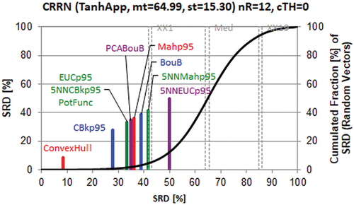
The Convex Hull algorithm defines the interpolation space as the smallest convex area containing the entire training set; hence, it can be challenging with increasing dimensions, i.e. it is a fine approximation, and the leading position is understandable henceforth. The Euclidean distance is sensitive to outliers i.e. its random character is understandable even when considering five neighbours.

It is much more difficult to define AD for quantitative structure–property relationship models of chemical reactions in comparison with standard QSAR/QSPR models because it is necessary to consider several important factors (reaction representation, conditions, reaction type, atom-to-atom mapping, etc.) [55].

Rakhimbekova et al. [55] have compared various AD definition methods for four types of reactions (Bimolecular nucleophilic substitution (SN2), Diels–Alder reactions (DA), Bimolecular elimination (E2) and Tautomerization). They have used four performance metrics and categorized the AD definition methods as i) machine learning technique-dependent AD definition methods, and universal AD definition methods ii) with optimized hyperparameters and iii) without the usage of hyperparameters. Finally, 16 method combinations were compared. The authors have properly realized that the situation is an MCDM one and introduced ‘zero’ models with best and worst performances. The transpose of their Table 3 [55] is suitable for an SRD analysis. Again, the selection of an appropriate gold standard is a sensitive decision. Fortunately, numerical optimal values are given in Table 3 of ref. [55] (OIR criterion, four values in line 19 of Table 3), and the hypothetical best values were selected in case of all other criteria (the maximum). The details can be found in the Rakhimbekova sheet of supplementary information.

Figure 7 suggests making three classes: recommendable techniques below SRD ≈ 30 (indicated by the dashed black vertical line) from RFR_VAR*_OIR to Leverage, NOT recommendable techniques above SRD ≈ 30 from RFR_VAR*_OD to GPR-AD*_OD and one forbidden method combination: 1-SVM*_OD. The latter one could not pass the randomization test, i.e. it cannot be distinguished from random ranking. The notation can be found in the Rakhimbekova sheet in supplementary information and in ref. [55].

Figure 7. Comparison of the methods for determining the applicability domain for four types of reactions, i.e. scaled sum of ranking difference (SRD) values between 0 and 100 (x and left y axes). Abbreviations can be seen in the text. The solid (black) line is an approximation by cumulated Gauss distribution to the discrete distribution of the simulated random numbers (500 000) given in relative frequencies, right y axis.

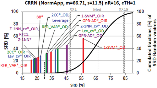
The large gap between SRD = 0 and SRD ≈ 25 suggests clearly that none of the examined method combinations are optimal, and better ones can be elaborated in the future.

It is obvious that the best performance parameter is the difference between RMSE of property prediction for reactions outside and within AD (OIR). This metric was first proposed by Sahigara et al. [54]. Namely, the best (first four) method combinations are based on OIR according to SRD analysis. The other parameter, though it is used multiple times, the outlier detection (OD, an analogue of balanced accuracy) is far inferior: OD is present in the last (worst) four combinations (Figure 7).

Naturally, another outcome might be expected, if the method is changed for the determination of AD, e.g. somewhat better results are expected if the k-nearest neighbour environment would increase from k= 1 to (say) five. However, the comparison is exhaustive—if one intends to tailor (or even to standardize) the determination of AD methods—only several combinations would suffice.

Discussion

Which algorithm(s), which performance parameters, which validation variants should be used—all constitute typical MultiCriteria Decision-Making (MCDM) problems and cannot be solved properly when neglecting the interplay of conflicting criteria.

It is known that machine learning approaches pioneered validation techniques: cross-validation variants, bootstrap, jackknife, randomization test and similar ones. Convolutional or deep neural networks cannot be validated in known ways: they cannot pass the randomization test, and changing even one pixel in the corner of the image deteriorates the licence plate recognition completely. My personal view is that deep learning is suitable for the rationalization of existing information (description, interpolation) but not for prediction (extrapolation). Hence, proper validation techniques should be elaborated urgently for different tasks, various problems, and specific datasets individually.

Validation aspects can be coded binarily with certain (slight or considerable) information loss. The loss is quantifiable by calculating uncertainties, confidence interval statistical testing and alike. SRD does not use binary coding, but rank transformation (RT); RT eliminates scaling problems at the expense of some information loss. The obvious coding for Applicability Domain (AD) is also binary: yes or no = in or out of AD.

Imbalanced datasets are quite common in drug design and medicinal chemistry. Balanced accuracy [56] was introduced as a performance metric to overcome biased classification. Balanced accuracy should be preferred over accuracy because the former performs similarly to accuracy on balanced datasets, but it still returns true model performance on imbalanced datasets. When performing MCDM analysis, balanced accuracy is only one of the conflicting factors, it exerts negligible effect to the fair method comparison; c.f. Rácz et al. who have compared 25 performance measures in multiclass situations [57]: accuracy and balanced accuracy did not exert significantly different outcomes in the case of the three different datasets examined.

Deep learning models, e.g. convolutional neural networks (CNNs), are considerably over-parameterized. They have many more weights to be fitted than the number of observations they were trained on. Consequently, CNN should be more prone to overfitting than their fully connected parallels. However, it has recently been shown that CNNs exhibit implicit self-regulation, which enhances their ability to better generalize [58]. This apparent contradiction can only be overcome if MCDM techniques are introduced in the validation step.

Conclusions and recommendations

The ordering based on sum of absolute values for ranking differences (SRD) is entirely general; it can be applied to evaluate and rank (i) modelling methods, (ii) variants of cross-validation, (iii) statistical tests, (iv) classification rates, v) information criteria, vi) methods determining the applicability domain and vii) performance parameters, as well.

Moreover, the evaluation, ordering and grouping have been completed in a reliable manner, in full conformity with the messages of the original authors.

However, the results of this work involve far-reaching consequences. Cross-validation is not one technique but a bunch of methods differing in algorithms, in aims, in predictive performances (in bias, variance and various degrees of freedom) and in implementations. Data structure also exerts a serious influence on the results of cross-validation. It is not sufficient to publish the name of the validation method; the next issues should also be given detailed algorithm, implementation and decision criteria.

The literature is full of contradictory statements, which are based on empirical evidence. Most scientists tend to accept experimental and empirical evidence as ‘truth’ without hesitation. The dissonance cannot be solved to search for new evidence and other datasets, recommending different practices, as the counterarguments can also be supported similarly. Multicriteria decision-making methods of model comparison, not utilized until now, are suitable to dissolve such discrepancies. Having not been biased by the conviction of the original authors, SRD can compare the methods and criteria in a fair way.

Reliable statistical tests (t-test, if the normality can be assumed, or Wilcoxon matched pair test, if distributional assumptions cannot be made) can determine whether the difference is significant between SRD values of models (methods, performance parameters, etc.) to be compared and those derived from simulation test by random numbers.

What is the recommended policy, if it is almost sure that the same techniques can be applied (or optimized) to be superior and far inferior? Use more variants of validation and cross-validation (>7) and compare criteria for a series of specific situations using a sum of ranking differences (search for consensus). The best validation method will be suitable in similar situations without completing all calculations, resampling, etc.

To obtain a reliable picture on which validation criteria can be used for a given modelling task (situation), at least four performance criteria must be checked: r²(training set), biased heavily upwards, Q²(leave-one-out), biased in similar direction but to less extent, Q²(bootstrap), biased heavily downwards and Q²(prediction set) biased downwards less than bootstrap. Prediction indicators for randomization tests cannot be used in comparison as they deteriorate the original modelling process. They are, however, useful in statistical testing, assuming a null hypothesis that the two groups (simulated with random numbers and the real one) stem from the same distribution, and rejection of the hypothesis, if the difference is significant. Williams-t-test seems to be suitable as it takes into account the cross-correlation of performance indicators.

Practitioners of Bayesian methods might experience disappointment that a simple fivefold cross-validation is generally better than the Bayesian information criterion when truly exhausting different situations.

Methods for the determination of the applicability domain have not been standardized yet, but some efforts are worth to think over: i) convex hull algorithm is to be preferred; ii) Random forest regression, in combination of the variance in the ensemble of predictions and of OIR criterion (‘out or in RMSE’ – the difference between RMSE of property prediction outside or within AD) is a good candidate, whereas support vector machine with outlier detection criterion is to be avoided for the validation of methods to determine the applicability domain.

Acknowledgements

Klára Kollár-Hunek’s help (in writing a Visual Basic macro for MS Excel) is gratefully acknowledged. The author thanks Dávid Bajusz and Anita Rácz for proofreading the manuscript.

Disclosure statement

No potential conflict of interest was reported by the author.

Supplementary material

Supplemental data for this article can be accessed at: https://doi.org/10.1080/1062936X.2023.2214871.

Additional information

Funding

This work was supported by the Ministry of Innovation and Technology of Hungary from the National Research, Development and Innovation Fund, financed under the K type funding scheme [OTKA K 134260].

References

- D.M. Hawkins, S.C. Basak, and D. Mills, Assessing model fit by cross-validation, J. Chem. Inf. Comput. Sci. 43 (2003), pp. 579–586. doi:10.1021/ci025626i.
- M. Gütlein, C. Helma, A. Karwath, and S. Kramer, A large-scale empirical evaluation of cross-validation and external test set validation in (Q)SAR, Mol. Inf. 32 (2013), pp. 516–528. doi:10.1002/minf.201200134.
- A. Rácz, D. Bajusz, and K. Héberger, Consistency of QSAR models: Correct split of training and test sets, ranking of models and performance parameters, SAR QSAR Env. Res. 26 (2015), pp. 683–700. doi:10.1080/1062936X.2015.1084647.
- K.H. Esbensen and P. Geladi, Principles of proper validation use and abuse of re-sampling for validation, J. Chemom. 24 (2010), pp. 168–187. doi:10.1002/cem.1310.
- P. Gramatica, Principles of QSAR models validation: Internal and external, QSAR Comb. Sci. 26 (2007), pp. 694–701. doi:10.1002/qsar.200610151.
- F. Westad and F. Marini, Validation of chemometric models—A tutorial, Anal. Chim. Acta 893 (2015), pp. 14–24. doi:10.1016/j.aca.2015.06.056.
- P. Gramatica and A. Sangion, A historical excursus on the statistical validation parameters for QSAR models: A clarification concerning metrics and terminology, J. Chem. Inf. Model. 56 (2016), pp. 1127–1131. doi:10.1021/acs.jcim.6b00088.
- P.J. Castaldi, I.J. Dahabreh, and J.P.A. Ioannidis, An empirical assessment of validation practices for molecular classifiers, Brief. Bioinf. 12 (2011), pp. 189–202. bbq073. doi:10.1093/bib/bbq073.
- M. Chatterjee and K. Roy, Application of cross-validation strategies to avoid overestimation of performance of 2D-QSAR models for the prediction of aquatic toxicity of chemical mixtures, SAR QSAR Environ. Res. 33 (2022), pp. 463–484. doi:10.1080/1062936X.2022.2081255.
- P. Gramatica, S. Cassani, P.P. Roy, S. Kovarich, C.W. Yap, and E. Papa, QSAR Modeling is not “push a button and find a correlation”: A case study of toxicity of (benzo-)triazoles on algae, Mol. Inform. 31 (2012), pp. 817–835. doi:10.1002/minf.201200075.
- P. Gramatica, External evaluation of QSAR models, in addition to cross-validation: Verification of predictive capability on totally new chemicals, Mol. Inform. 33 (2014), pp. 311–314. doi:10.1002/minf.201400030.
- V. Consonni, D. Ballabio, and R. Todeschini, Evaluation of model predictive ability by external validation techniques, J. Chemom. 24 (2010), pp. 194–201. doi:10.1002/cem.1290.
- N. Chirico and P. Gramatica, Real external predictivity of QSAR models: How to evaluate it? Comparison of different validation criteria and proposal of using the concordance correlation coefficient, J. Chem. Inf. Model. 51 (2011), pp. 2320–2335. doi:10.1021/ci200211n.
- V. Pandit and B. Schuller, The many-to-many mapping between the concordance correlation coefficient, and the mean square error, (1 Jul 2020). https://arxiv.org/pdf/1902.05180.pdf.
- S. Shayanfar and A. Shayanfar, Comparison of various methods for validity evaluation of QSAR models, BMC Chem. 16 (2022), Article Number: 63. doi:10.1186/s13065-022-00856-4.
- M.N. Triba, L. Le Moyec, R. Amathieu, C. Goossens, N. Bouchemal, P. Nahon, D.N. Rutledge, and P. Savarin, PLS/OPLS models in metabolomics: The impact of permutation of dataset rows on the k-fold cross-validation quality parameters, Mol. BioSyst. 11 (2015), Article Number: 13. doi:10.1039/C4MB00414K.
- A. Rakhimbekova, T.N. Akhmetshin, G.I. Minibaeva, R.I. Nugmanov, T.R. Gimadiev, and T.I. Madzhidov, Cross-validation strategies in QSPR modelling of chemical reactions, SAR QSAR Environ. Res. 32 (2021), pp. 207–219. doi:10.1080/1062936X.2021.1883107.
- K. Héberger and K. Kollár-Hunek, Comparison of validation variants by sum of ranking differences and ANOVA, J. Chemom. 33 (2019), pp. 1–14. Article number: e3104. doi:10.1002/cem.3104.
- C. Rücker, G. Rücker, and M. Meringer, y-Randomization and its variants in QSPR/QSAR, J. Chem. Inf. Model. 47 (2007), pp. 2345–2357. doi:10.1021/ci700157b.
- R. Bro, K. Kjeldahl, A.K. Smilde, and H.A.L. Kiers, Cross-validation of component models: A critical look at current methods, Anal. Bioanal. Chem. 390 (2008), pp. 1241–1251. doi:10.1007/s00216-007-1790-1.
- Available at http://wiki.eigenvector.com/index.php?title=Using_Cross-Validation (accessed March 04, 2023).
- P. Filzmoser, B. Liebmann, and K. Varmuza, Repeated double cross validation, J. Chemom. 23 (2009), pp. 160–171. doi:10.1002/cem.1225.
- D. Baumann and K. Baumann, Reliable estimation of prediction errors for QSAR models under model uncertainty using double cross-validation, J. Cheminform. 6 (2014), Article Number: 47. doi:10.1186/s13321-014-0047-1.
- Y. Xu and R. Goodacre, On splitting training and validation set: A comparative study of cross-validation, bootstrap and systematic sampling for estimating the generalization performance of supervised learning, J. Anal. Testing 2 (2018), pp. 249–262. doi:10.1007/s41664-018-0068-2.
- L. Shi, J.A. Westerhuis, J. Rosé, R. Landberg, and C. Brunius, Variable selection and validation in multivariate modelling, Bioinformatics 35 (2019), pp. 972–980. doi:10.1093/bioinformatics/bty710.
- A. Kozak and R. Kozak, Does cross-validation provide additional information in the evaluation of regression models? Can. J. Forest Res. 33 (2003), pp. 976–987. doi:10.1139/x03-022.
- S. Guo, T. Bocklitz, U. Neugebauer, and J. Popp, Common mistakes in cross-validating classification models, Anal. Meth. 9 (2017), pp. 4410–4417. doi:10.1039/C7AY01363A.
- A. Rácz, D. Bajusz, and K. Héberger, Modelling methods and cross-validation variants in QSAR: A multi-level analysis, SAR QSAR Environ. Res. 29 (2018), pp. 661–674. doi:10.1080/1062936X.2018.1505778.
- D. Kovács, P. Király, and G. Tóth, Sample-size dependence of validation parameters in linear regression models and in QSAR, SAR QSAR Environ. Res. 32 (2021), pp. 247–268. doi:10.1080/1062936X.2021.1890208.
- S.Y. Ho, K. Phua, L. Wong, and W.W. Bin Goh, Extensions of the external validation for checking learned model interpretability and generalizability, Patterns 1 (2020), Article Number: 100129. doi:10.1016/j.patter.2020.100129.
- D. Chicco, M.J. Warrens, and G. Jurman, The coefficient of determination R-squared is more informative than SMAPE, MAE, MAPE, MSE and RMSE in regression analysis evaluation, PeerJ. Comp. Sci. 7 (2021), pp. e623. doi:10.7717/peerj-cs.623.
- OECD, Guidance document on the validation of (Quantitative) Structure-Activity Relationship [(Q)SAR] models, OECD Series on Testing and Assessment, No. 69, OECD Publishing, Paris, 03 September 2014.
- NAFTA WGP, (Quantitative) Structure Activity Relationship [(Q)SAR] guidance document. NAFTA Technical Working Group on Pesticides. November, 2012. Available at https://www.epa.gov/sites/default/files/2016-01/documents/qsar-guidance.pdf.
- M. Pavan, Total and partial ranking methods in chemical sciences, Ph.D. Theses, University of Milano–Bicocca, Italy, 2003.
- T.-C. Wang and H.-D. Lee, Developing a fuzzy TOPSIS approach based on subjective weights and objective weights, Expert Syst. Appl. 36 (2009), pp. 8980–8985. doi:10.1016/j.eswa.2008.11.035.
- K. Héberger, Sum of ranking differences compares methods or models fairly, TrAC Trends Anal. Chem. 29 (2010), pp. 101–109. doi:10.1016/j.trac.2009.09.009.
- W. Nowik, S. Héron, M. Bonose, and A. Tchapla, Separation system suitability (3S): A new criterion of chromatogram classification in HPLC based on cross-evaluation of separation capacity/peak symmetry and its application to complex mixtures of anthraquinones, Analyst 138 (2013), pp. 5801–5810. doi:10.1039/c3an00745f.
- S. Kovačević, M. Karadžić, S. Podunavac-Kuzmanović, and L. Jevrić, Binding affinity toward human prion protein of some anti-prion compounds—Assessment based on QSAR modeling, molecular docking and non-parametric ranking, Eur. J. Pharm. Sci. 111 (2018), pp. 215–225. doi:10.1016/j.ejps.2017.10.004.
- B. Brownfield and J.H. Kalivas, Consensus outlier detection using sum of ranking differences of common and new outlier measures without tuning parameter selections, Anal. Chem. 89 (2017), pp. 5087–5094 and 960. doi:10.1021/acs.analchem.7b00637.
- F. Andrić and K. Héberger*, Towards better understanding of lipophilicity: Assessment of in silico and chromatographic log P measures for pharmaceutically important compounds by nonparametric rankings, J. Pharm. Biomed. Anal. 115 (2015), pp. 183–191. doi:10.1016/j.jpba.2015.07.006.
- N.M. Bhatt, V.D. Chavada, M. Sanyal, and P.S. Shrivastav, Influence of organic modifier and separation modes for lipophilicity assessment of drugs using thin layer chromatography indices, J. Chromatog. A 1571 (2018), pp. 223–230. doi:10.1016/j.chroma.2018.08.009.
- K. Ciura, J. Fedorowicz, F. Andrić, K.E. Greber, A. Gurgielewicz, W. Sawicki, and J. Saczewski, Lipophilicity determination of quaternary (Fluoro)quinolones by chromatographic and theoretical approaches, Int. J. Mol. Sci. 20 (2019), Article number 5288. doi:10.3390/ijms20215288.
- B.R. Sziklai, Ranking institutions within a discipline: The steep mountain of academic excellence, J. Inform. 15 (2021), pp. 101133. doi:10.1016/j.joi.2021.101133.
- R.A. Miranda-Quintana, D. Bajusz, A. Rácz, and K. Héberger, Extended similarity indices: The benefits of comparing more than two objects simultaneously. Part 1: Theory and characteristics, J. Cheminf. 13 (2021), Article Number: 32. doi:10.1186/s13321-021-00505-3.
- R.A. Miranda-Quintana, A. Rácz, D. Bajusz, and K. Héberger, Extended similarity indices: The benefits of comparing more than two objects simultaneously. Part 2: Speed, consistency, diversity selection, J. Cheminf. 13 (2021), Article Number: 33. doi:10.1186/s13321-021-00504-4.
- X. Chen, Y. Xu, L. Meng, X. Chen, L. Yuan, Q. Cai, W. Shi, and G. Huang, Non-parametric partial least squares–discriminant analysis model based on sum of ranking difference algorithm for using electronic tongue data identify tea grade using e-tongue data, Sens. Actuators B Chem. 311 (2020), Article Number: 127924. doi:10.1016/j.snb.2020.127924.
- J. Lourenco and L. Lebensztajn, Post-pareto optimality analysis with sum of ranking differences, IEEE Trans. Magn. 54 (2018), pp. 1–10. Article Number: 8202810. doi:10.1109/TMAG.2018.2836327.
- T. Hastie, R. Tibshirani, and J. Friedman, The elements of statistical learning: Data mining, inference, and prediction, in Chapter 8 Model Inference and Averaging, 2nd ed., Springer, New York, 2009, pp. 261–294.
- K. Héberger and K. Kollár-Hunek, Sum of ranking differences for method discrimination and its validation: Comparison of ranks with random numbers, J. Chemom. 25 (2011), pp. 151–158. doi:10.1002/cem.1320.
- J.J. Kraker, D.M. Hawkins, S.C. Basak, R. Natarajan, and D. Mills, Quantitative structure-activity relationship (QSAR) modeling of juvenile hormone activity: Comparison of validation procedures, Chemom. Intell. Lab. Syst. 87 (2007), pp. 33–42. doi:10.1016/j.chemolab.2006.03.001.
- H.R. Cederkvist, A.H. Aastveit, and T. Næs, A comparison of methods for testing differences in predictive ability, J. Chemom. 19 (2005), pp. 500–509. doi:10.1002/cem.956.
- R. Mac Nally, R.P. Duncan, J.R. Thomson, and J.D.L. Yen, Model selection using information criteria, but is the “best” model any good? J. Appl. Ecol. 55 (2018), pp. 1441–1444. doi:10.1111/1365-2664.13060.
- D. Toher, G. Downey, and T.B. Murphy, A comparison of model-based and regression classification techniques applied to near infrared spectroscopic data in food authentication studies, Chemom. Intell. Lab. Syst. 89 (2007), pp. 102–115. doi:10.1016/j.chemolab.2007.06.005.
- F. Sahigara, K. Mansouri, D. Ballabio, A. Mauri, V. Consonni, and R. Todeschini, Comparison of different approaches to define the applicability domain of QSAR models, Molecules 17 (2012), pp. 4791–4810. doi:10.3390/molecules17054791.
- A. Rakhimbekova, T.I. Madzhidov, R.I. Nugmanov, T.R. Gimadiev, I.I. Baskin, and A. Varnek, Comprehensive analysis of applicability domains of QSPR models for chemical reactions, Int. J. Mol. Sci. 21 (2020), Article Number: 5542. doi:10.3390/ijms21155542.
- K.H. Brodersen, C.S. Ong, K.E. Stephan, and J.M. Buhmann, The balanced accuracy and its posterior distribution, Proceedings - 20th International Conference on Pattern Recognition, Istanbul, Turkey, 2010, No. 5597285, pp. 3121–3124 doi:10.1109/ICPR.2010.764.
- A. Rácz, D. Bajusz, and K. Héberger, Effect of dataset size and train/test split ratios in QSAR/QSPR multiclass classification, Molecules 26 (2021), Article Number 1111. doi:10.3390/molecules26041111.
- C.H. Martin and M.W. Mahoney, Implicit self-regularization in deep neural networks: Evidence from random matrix theory and implications for learning, J. Mach. Learn. Res. 22 (2021), pp. 1–73.