What is the ecotoxicity of a given chemical for a given aquatic species? Predicting interactions between species and chemicals using recommender system techniques

ABSTRACT

Ecotoxicological safety assessment of chemicals requires toxicity data on multiple species, despite the general desire of minimizing animal testing. Predictive models, specifically machine learning (ML) methods, are one of the tools capable of solving this apparent contradiction as they allow to generalize toxicity patterns across chemicals and species. However, despite the availability of large public toxicity datasets, the data is highly sparse, complicating model development. The aim of this study is to provide insights into how ML can predict toxicity using a large but sparse dataset. We developed models to predict LC50-values, based on experimental LC50-data covering 2431 organic chemicals and 1506 aquatic species from the ECOTOX-database. Several well-known ML techniques were evaluated and a new ML model was developed, inspired by recommender systems. This new model involves a simple linear model that learns low-rank interactions between species and chemicals using factorization machines. We evaluated the predictive performances of the developed models based on two validation settings: 1) predicting unseen chemical-species pairs, and 2) predicting unseen chemicals. The results of this study show that ML models can accurately predict LC50-values in both validation settings. Moreover, we show that the novel factorization machine approach can match well-tuned, complex, ML approaches.

KEYWORDS:

• Machine learning
• modelling
• aquatic toxicity
• species sensitivity
• prediction
• LC50

Introduction

Identification of chemical hazards is essential to estimate and manage the risks of exposure of biota to chemicals [1]. To date, hazard assessment has been typically performed on the basis of experimental toxicity data that is generated in a laboratory setting using test animals. Such toxicity tests consist of exposing species to various concentrations of the chemical of interest and evaluate the toxicity over varying periods of time. Large numbers of chemicals are being developed and brought to the market. However, only a limited amount of experimental toxicity data is typically available due to time restrictions and costs associated with these experiments, as well as ethical considerations. Accordingly, the hazards of many ‘new’ chemicals are insufficiently quantified, resulting in potential risks for the environment. To speed up and elaborate the hazard assessment, environmental hazard assessment would benefit from accurate predictive models as an alternative to animal experiments [2].

Traditionally, so-called QSAR (Quantitative Structure-Activity Relationships) models have been developed to predict aquatic toxicity, as for example the suite of models ECOSAR [3]. Within ECOSAR various sub-models have been developed based on linear regressions for different chemical functional classes and animal species i.e. algae, daphnia and fish. In addition, more recent developments focus on machine learning specifically. Machine learning methods are mathematical algorithms that can learn complex patterns from large data sets. These machine learning methods can thus learn from existing toxicity experiments by relating the underlying testing conditions to the biological endpoint. The learned patterns can subsequently be used to predict biological responses of animal species exposed to new chemicals. Although the concept of applying machine learning to predict biological toxicity is not new [4–8], many modelling studies use a custom dataset that has been carefully curated for a particular species and/or a particular group of chemicals. However, consequently these models may not generalize well to new prediction settings.

Large public datasets are alleviating this problem, for example the TOX21 and Oral toxicity collaboration [9,10]. In this context, neural networks are usually found to be the most accurate modelling approach [11,12]. A vast majority of the research is focused on models for a single response such as LC50, or on modelling various different responses at a time: LC50, EC50, NOEC, etc. Models for multiple responses are often called multitask models [11–17]. Researchers and regulators have recognized the importance of building models for toxicity prediction over multiple species, which range up to a couple to hundreds of species [18–25]. However, even though many different species and chemicals are included in the data sets, the data is highly sparse. More specifically, an overwhelming majority of the chemicals has been tested on a few, or even only a single species. In addition, some species are widely used as test species for a variety of chemicals, whereas other species are hardly ever tested. This is mainly caused by regulatory data requirements, available standardized test guidelines, and standardized test setups offered by commercial testing laboratories for practical purposes (e.g. REACH legislation EC/1907/2006, OECD TG 201–203, and many others). In general, data sparsity complicates accurate model predictions. Sparsity is a good candidate for approaches based on transfer learning [26–28], because the large data set can be used to share information across species and chemicals.

The problem of training a machine learning model for ecotoxicity prediction can be considered as an instance of pairwise-learning, which has already been studied in various research fields. In pairwise learning, each input is viewed as a pair of objects x = (s, c), which in the context of ecotoxicity prediction could be a species s ∈ S and a chemical c ∈ C. The task is to predict new toxicity assessments y = f (x) for new species and chemical pairs. In ecotoxicity, including both chemical and species features is essential. The idea that different chemicals will be more or less toxic is mechanistically grounded in the various mechanisms of action that can be initiated by different chemical structures, or by the presence of specific chemical (sub)structures. Similarly, different species will react differently to a chemical exposure, which is shown in an overview of mechanistical, and evolutionary reasons that lead to different sensitivity of different species [29]

Pairwise learning has been widely applied within recommender systems, as these have a long history of predicting (user, item)-interactions [30,31]. It is also expected that modelling results can improve, or become more robust when all results for available species and chemical combinations are used to train models, instead of using only toxicity data for a single species, or disregard species differences within a group of species. In this context, two main approaches have been taken in the present study. The first approach is collaborative filtering [32], in which recommendations are based on how users and items have interacted without any additional knowledge of the users or the items. The second approach is content-based filtering [33], in which user and item features are used to recommend items to a particular user. In the context of toxicity, users can be interpreted as species, and items can be interpreted as chemicals. Generally, simple baselines in collaborative filtering work very well for pairwise learning problems, unless predictions are required for items with very few interactions [34,35]. In those cases, hybrid models can prove to be beneficial, incorporating both collaborative filtering and content-based filtering [35,36]. This approach is also popular in closely related drug-target interaction prediction [37–41] and there are many successful applications of collaborative filtering [42–45].

To the best of our knowledge, such pairwise-learning approaches have not yet been applied to predict toxicity for aquatic species and chemical interactions. We develop a simple linear model extended with interactions based on well-established research in recommender systems, and compare it to other machine learning methodologies, including random forests and neural networks. The aim of this study is to provide insights into how machine learning can predict toxicity using a large but sparse data set of LC50 values with a wide range of organic chemicals and aquatic species, covering various exposure durations. For this purpose, we used the ECOTOX database to derive a set of experimental LC50 measurements from a wide variety of chemicals, animal species and exposure durations.

Methods

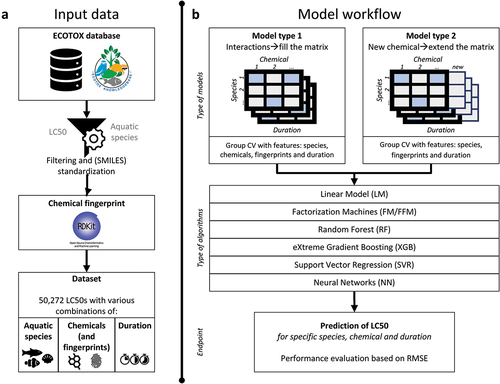
The study approach consists of various steps that are represented in Figure 1. First, toxicity data were collected and curated to generate a data set with experimental LC50s for various aquatic species, chemicals, and exposure duration combinations (Figure 1(a)). Second, this data set was used to train and validate the machine learning models (Figure 1(b)). The performances of various machine learning algorithms have been compared based on RMSE. Details about the modelling approach, including data splitting and model algorithm optimization are described in the following sections. All scripts used for data curation and model training have been made available via GitHub (https://github.com/majuvi/predictive_toxicology).

Figure 1. Overall summary of the study approach including data and modelling workflow.

Data set

ECOTOX database

In the present study, we use the ECOTOX database [46] to derive a data set with multiple species and toxicity values from exposure to multiple chemicals (Figure 1(a)). To the best of our knowledge, the ECOTOX database is the largest publicly accessible database containing experimental measurements of biological endpoints relevant to ecotoxicity. The ECOTOX database consists of the results of experimental toxicity experiments on aquatic and terrestrial species. Chemicals used in the experiments are characterized by their Chemical Abstract Service (CAS) number which was coupled by us to a Simplified Molecular-Input Line-Entry System (SMILES) representation of the chemical structure. For each experiment, a test organism is reported which is defined using the taxonomic species classification, and the corresponding test duration is reported. Finally, for each experiment, the studied biological endpoints are reported.

In the present study, we extracted the ECOTOX database [46], version 15 September 2022, and curated the data on various elements as follows: i) endpoints and effects were limited to LC50-values and mortality, ii) organism habitat was limited to water, iii) we excluded field experiments, iv) we excluded non-aquatic exposure types, e.g. via injection or exposure via food, v) we excluded data for which no exposure concentration or duration was reported, i.e. NR or a concentration or duration of 0, or where reported exposure concentrations or durations were ambiguous (‘>’, ‘<’ or ‘~’), vi) we limited the data to short-term durations, including only measurements of in between 1 and 168 hours., corresponding to 0–7 days. Alternative exposure durations that could not unambiguously be converted to hours or days were excluded, like larva to subadult, emergence, fry, etc. In addition, vii) we limited the data to relevant exposure concentration units that are related to aquatic exposure (like ng/mL or ppm) and could be easily converted to a common unit (mg/L). Accordingly, we for instance excluded measurements reported in molar mass or acid equivalents. Finally, viii) we only included data with an exposure concentration equal to or above 1 pg/L and equal to or below 10 g/L.

The CAS-numbers in the ECOTOX database are the chemical identifiers and were linked with SMILES using a list of the US-EPA [47]. We standardized and neutralized these SMILES using the QSAR ready workflow [48] of the open-source platform KNIME to generate QSARready-SMILES, which were then used to generate the chemical features. With this approach, UVCBs/mixtures and inorganics, including metals, were excluded from the dataset. In addition, we manually filtered chemicals with a QSARready-SMILES, that represent (organic) metal salts like: cadmium (Cd), cobalt (Co), chromium (Cr), copper (Cu), iron (Fe), mercury (Hg), nickel (Ni), lead (Pb), etc.

The final data set consisted of 2608 different chemicals based on CAS-number, which have 2431 different QSARr-SMILES, 1506 different species and 52272 experiments reporting LC50 values (see Supplemental Material). It should be noted that some chemicals identified by unique CAS-numbers can have an exact same QSARr-SMILES. Chemicals can for instance have a different salt coupled to their main chemical structure (e.g. 2,2-Dichloropropanoic acid; CAS = 75-99-0 and 2,2-Dichloropropanoic acid sodium salt; CAS = 127-20-8), or can include specific isomers with a similar standardized and neutralized QSARr-SMILES. As it is in general within this selected dataset not the salt structure that determines the toxicological effects, but the organic counterpart, it is the organic element we have used as input for the model development and calculation of chemical fingerprints.

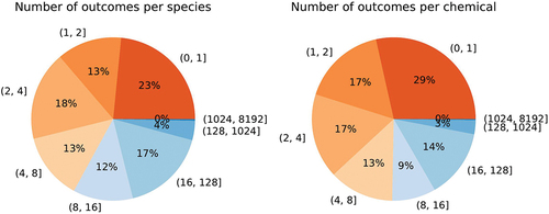
A noteworthy feature is the sparsity of data. Only 14,449 (species, chemical)-pairs have one or more toxicity outcomes, whereas we have 1506 different species and 2431 different chemicals based on unique QSARr-SMILES, resulting in 3,661,086 possible combinations. Hence, only 0.4% of all possible species and chemical pairs have some outcomes. Likewise, while there are many species and many chemicals, most of them have very few outcomes as illustrated in Figure 2. There are on average 35 outcomes per species, with median 4, min 1, and max 5005. There are on average 22 outcomes per chemical, with median 3, min 1, and max 1841. For ecotoxicological risk assessment purposes it would be much more beneficial to have the experimental data being distributed more evenly over both species and chemicals, i.e. not have one chemical tested 1841 times, or having the majority of all tests being performed with the same species over and over again, as a single species will not give a good representation of the toxic effect of a chemical on ecosystems. A priori it is impossible to say how representative a single species, such as the much used Pimephales promelas – the fathead minnow, will be for the ecosystems we intend to protect by doing chemical risk assessment.

Figure 2. Pie charts of the data set sparsity illustrate that most species and chemicals have few outcomes. Most species and chemicals have less than 4 experiments that deliver LC50 values.

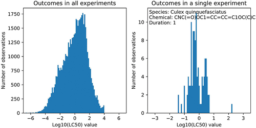
For modelling purposes, the LC50 values (in mg/L) were log-transformed, so Log10(LC50) was defined as the predicted outcome. Figure 3 illustrates the approximately log-normal distribution of the outcomes. The unit of the test durations reported for each outcome was converted into hours. Almost all of the test durations fell into discrete values 1 h (314), 3 h (618), 6 h (810), 12 h (634), 24 h (14949), 48 h (10762), 72 h (2857), 96 h (20324), 120 h (291), 168 h (713) where the number of experiments is in parenthesis, with all other durations having fewer than 200 experiments. We aggregated these few test durations into the closest discrete value. The discrete durations were treated as a categorical variable in a linear model to enable the learning of a non-linear relationship of test duration with LC50 values.

Figure 3. The distribution of all LC50 toxicity values in log10 mg/L (left) and repetitions within the most tested experimental setting in the data set.

Feature representation

The QSARr-SMILES representation of each chemical was used to define the chemical features. Specifically, chemical features were defined as the 1024-count-based Morgan fingerprint calculated from the SMILES representation using the Python package rdkit with a radius of 2 [49]. This resulted in a sparse feature vector for every chemical. Every dimension was first log (1+x)-transformed and then minmax-scaled, since this achieved a better accuracy than a non-transformed feature vector. Feature transforms are often used to improve the performance of algorithms such as ridge regression, support vector machine, and neural networks. The chemical fingerprint is a numerical feature with high sparsity, i.e. many of the entries are 0. In addition to the chemical features, we also defined a one-hot encoded chemical indicator with a 2431 length vector, based on the unique QSARr-SMILES. The ‘chemical’ indicator is a categorical feature with high cardinality, i.e. a long vector of 0s including only one entry with 1.

For every species, we defined a one-hot encoded indicator of the species as a 1506-length vector. Like the ‘chemical’ indicator, the ‘species’ indicator is a categorical feature with high cardinality. In this study we did not have other features that describe the species. Taxonomic information, body weights or genome similarities could for example be considered as additional information, in the same way the chemical fingerprint is included in addition to the chemical indicator. In total, the data provides us with four-feature vectors: the ‘chemical’ indicator, the chemical fingerprints, the species indicator, and the duration.

Experimental variability from repeated measurements

The dataset employed in the present study is subject to biological variability as well as experimental variability due to different experimental setups or personnel. This means that the same experiment, i.e. the same chemical, species, and duration, can result in varying LC50 values. As a consequence, it is impossible for a machine learning algorithm, or any computational model for that matter, to achieve a perfect prediction. Therefore, we quantified the variability from repeated experimental settings. Repeated outcomes can be used to quantify the amount of noise in the data, which can be experimental error or natural variation caused by heterogeneous populations [50].

To this end, we define an experimental setting as a triplet x = (s, c, d) with species s ∈ S, chemical c ∈ C, and test duration d ∈ D. Only some of these experimental settings have measured LC50 toxicity values y. The data set can contain repeated outcomes at a given experimental setting. We denote the number of outcomes at a given experimental setting as N_s,c,d ∈ {0}∪ ℕ. The sample size is the total number of outcomes N = ∑_s,c,d N_s,c,d . This is illustrated in Figure 3 for a single experimental setting with many repetitions. Denote the outcome of an experiment y_s,c,d,i = µ_s,c,d + ϵ_s,c,d,i. The ’true toxicity’ µ_s,c,d is the expected toxicity outcome and the ’noise’ ϵ_s,c,d is the deviation in a single outcome. This noise is spread according to the standard deviation σ_s,c,d . Assuming for simplicity that the noise is homogeneous across experimental settings σ = σ_s,c,d, the noise can be calculated using standard statistics.

${\hat{\mu }}_{s,c,d}=\frac{1}{N\left(s,c,d\right)}\sum _{i=1}^{N\left(s,c,d\right)}{y}_{s,c,d,i}$

We directly model the sample mean of each experimental setting and calculate the residual sum of squares between the predicted mean and the outcomes. This model has as many free parameters $d=\sum _{s,c,d}\mathbb{I}\left(N_{s,c,d}>0\right)$ as there are experimental settings with at least one outcome. An estimate of the standard deviation is the square root of the residual sum of squares divided by the degrees of freedom:

${\sigma }^2=\frac{1}{N-d}\sum _{s,c,d}{\sum }_{i=1}^{N\left(s,c,d\right)}{\left(y_{s,c,d,i}-{\hat{\mu }}_{s,c,d}\right)}^2$

The predictions of a machine learning model y = f (x) takes an experimental setting x = (s, c, d) as the input. A ’perfect’ model that minimizes the Root Mean Squared Error (RMSE) predicts the mean of each experimental setting correctly in test data. The amount of noise therefore sets a lower threshold on the RMSE of any model.

Validation

Denote the set of experimental settings as the cartesian product of species, chemicals, and duration X = S × C × D and the toxicity outcomes as a set Y. Our goal is to learn a function f : X → Y from the training set X_train, such that it can correctly predict the mean for a new experiment x ∈X_test. Assume the training set has species S_train and chemicals C_train, which may be a subset of all species and chemicals. We consider two different prediction settings, depending on whether the chemical has already been tested or not. The first setting considers the prediction of new species-chemical interactions, where both species and chemical have been used in the training data whilst their combination has not been. The second setting considers prediction for new chemicals that have never been used in the training process, regardless of the tested species. Thus, the first validation setting evaluates the models’ performances when predicting LC50 values of chemicals that have previously been tested on different species. On the contrary, the purpose of the second validation setting was to evaluate the models’ performance when predicting LC50 values of unseen chemical, which is particularly relevant for newly developed chemicals that have not been tested before. We define the train/test set split as follows and these two settings are illustrated in Figure 4:

Figure 4. Data set split into training and test sets can be visualized as partitioning a 3D array. In the first validation setting, groups that are split either into train or test are defined by (species, chemical)-pairs. In the second validation setting, these groups are defined by chemicals.

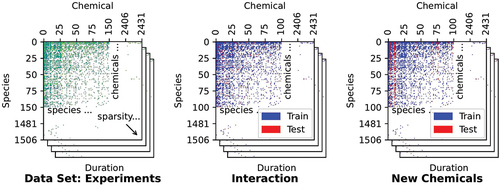
1. Split the species-chemical pairs into mutually exclusive training and test sets (S × C) = (S × C)_train ∪ (S × C)_test. Then define: x_s,c,d,i ∈ X_train if (s, c) ∈ (S × C)_train and x_s,c,d,i ∈ X_test if (s, c) ∈ (S × C)_test. This setting evaluates the model on new species and chemical interactions.

2. Split the chemicals C = C_train∪ ∈ C_test into mutually exclusive train and test sets. Then define: x_s,c,d,i ∈ X_train if c ∈ C_train and x_s,c,d,i ∈ X_test if c ∈ C_test. This setting evaluates the model on new chemicals.

It must be noted that the test/train split is based on the (species, chemical)-pairs or chemicals, and not on the test duration or a random split. The reason for this is that we do not want to use a test set that contains chemical-species combinations that are also present in the training dataset. We believe that this is not fully representative of the current risk assessment, as risk assessors are typically interested in predicting LC50 values if no information is available on a particular chemical-species combination (validation setting 1), or if a completely new chemical is considered for which no toxicity data is available at all (validation setting 2). Thus, if a chemical-species combination has previously been tested, there is usually no need to predict LC50 values for the same combination, possibly with a different exposure duration. Hence, in order to avoid overestimating our model’s performance for those applications, we decided on the grouped cross-validation strategy described above.

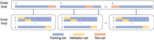
For the first setting (i.e. interactions) we use the duration, species indicator, the chemical indicator, and the chemical fingerprint as features to predict toxicity. For the second setting (i.e. new chemicals), we use the duration, species indicator and the chemical fingerprint as features. Due to the varying test durations and the repeated measurements, we use five-fold nested grouped cross-validation (Figure 5). The cross-validation data sets are defined by species-chemical interactions in the first setting and ‘chemical’ in the second setting. It must be noted that both validation settings ensure that experimental results obtained from the same study (e.g. same chemical, same species, various durations), are either all in the training set or the test set. The final model performance is reported as the average RMSE over the five test sets (see Figure 5).

Figure 5. Overview of the nested 5-fold grouped cross-validation procedure employed in this study. First, the data set is split into training and test folds: a model is trained on each fold, using training data without seeing the test data. To find optimal hyperparameters, this training set is further split into training and validation sets using the same cross-validation strategy.

As an additional way of interpreting the LC50 values predicted by the proposed linear model, we grouped the predicted LC50 values into classification bins. Classifications of chemical toxicity is often necessary for the classification and labelling of chemicals. To this end, we defined five different toxicity classes [mg/L] that are also often used for regulatory purposes: (0, 1], (1,10], (10,100], (100,1000], (1000, ∞). Each predicted LC50 value was put into the corresponding classification bin, and the confusion matrices resulting from the first and the second validation setting were reported. Furthermore, three metrics were used to quantify the classification quality: the precision, recall and F1-score.

Models

In the present study, we evaluated various machine learning models and compared the results to our proposed models, which are described below.

Null model (NULL)

The null model is a simple baseline model that gives the same output: the mean LC50 value of the training set.

Linear model (LM)

We implemented least squares regression with L2 regularization, also known as Ridge Regression, using the implementation in scikit-learn [51]. This is a simple, fast, and easily interpretable model. The model is a linear equation of the features. A manually specified feature transformation can be used to learn non-linear relationships and interactions with this model. We use this model to illustrate a sequence of increasingly elaborate models and show how the predictive accuracy increases. The model has only one hyperparameter: λ regularization penalty.

Factorization machines (FM)

Factorization machines are simple but effective algorithms that extend the linear model by allowing interaction terms. The model is a simple linear equation of the features and all pairwise interactions between the features, which are learned as a low-rank representation [35]. The algorithm is especially useful for highly sparse data with interactions, typical in recommender systems [52]. When the model includes more than two inputs (besides the species and the chemical), e.g. duration and chemical fingerprint, we use Field-Aware Factorization machines.

The simplest model uses no features at all and equals matrix completion popular in collaborative filtering [34]. The matrix of partially observed LC50 values is factorized as a product of two low-rank matrices corresponding to species and chemicals. When we include chemical fingerprints into this model, we get a hybrid recommender system with content features. This assumes that the chemical fingerprint can be used to learn the toxicity of a chemical for different species, using low-rank matrices. The low-rank matrices correspond to an implicit assumption that species are similar to each other, which allows sharing of information between species. The chemical features are expected to help the collaborative filtering approach when we predict new chemicals with few or no outcomes.

The algorithm has two important hyperparameters: λ regularization penalty and k the number of iterations, which was set with early stopping. We found that the number of latent dimensions d = 256 could be set to a fixed high value when the model was carefully regularized.

Random forest (RF)

Random forest [53] is a popular algorithm based on bagging of multiple decision trees trained on different subsets of the data. The algorithm has been widely applied in many fields, since it is quite robust to different data sets and often requires little tuning, easily resulting in good predictions.

We optimized over multiple hyperparameters to possibly benefit from adjusting the level of randomness and regularization: the number of features to consider when looking for the best split, the minimum number of samples required to be at a leaf node, the number of features to consider when looking for the best split, whether bootstrap samples or the full data set is used when building trees, the number of samples drawn to train each base estimator, and the number of trees. As expected, the model kept improving with more trees up to around k = 300.

eXtreme gradient boosting (XGB)

Gradient boosted decision trees [54] are another popular algorithm, based on boosting simpler decision trees that incrementally improves the model. We used the XGBoost implementation that scales well for large data sets [55]. The algorithm has found many applications and it is quite robust to different data sets and hyperparameter combinations. Due to the greedy nature of the algorithm, at minimum the number of trees must be set to avoid overfitting the training data.

We again optimized over multiple hyperparameters to adjust the level of randomness and regularization: the depth of the trees, L2 regularization penalty term on the weights, the minimum loss reduction required to make a further partition on a leaf node of the tree, the fraction of the training instances sampled for each tree, and the number of trees set by early stopping. As expected, the model kept improving up to an optimal number of trees k, after which the error started to increase, strongly depending on the prediction setting.

Support vector regression (SVR)

Support Vector Regression is a traditional machine learning algorithm, which is popular and widely applied. The algorithm can learn highly complex non-linear functions through the similarity between a new data point and the training data using the Radial Basis Function (RBF) kernel. However, the algorithm does not scale well in the number of samples because the training time is more than quadratic. First, we tested if the fit time can be improved by using the Nyström method for kernel approximation [56], but the first setting required the full solution. Some hyperparameter combinations took days to fit a single model. The implementation in scikit-learn is a wrapper around the well-tested liblinear for linear models [57] and libsvm for non-linear models [58].

The model has two hyperparameters that we found very important: λ regularization penalty and γ the width of the RBF kernel.

Neural networks (NN)

Neural Networks (NN) are also traditional algorithms that have become very popular, especially by the use of deep Neural Networks (dNN) for complex problems [59]. Recent improvements in computing power and algorithms have resulted in large improvements in some fields [60]. Deep neural networks are beneficial for problems where the data set is large and there is a hierarchical structure where complex concepts are incrementally built from simple ones, such as in computer vision. These methods are now also popular in toxicology where the chemical structure might be expected to behave similarly. However, data set properties, neural network architecture, hyperparameter choices, and the optimization method can result in different performances, necessitating very careful tuning, which can be tedious and time-consuming.

We tried different architectures with different width of hidden layers, depth of hidden layers, activation functions, and adjusting regularization with dropout and l2 weight penalty. We also tried different learning rates, optimization methods and adjusting the learning rate with weight decay, but tensor flow defaults already resulted in a well optimized model.

Hyperparameter tuning

For hyperparameter tuning in training data, we used nested 5-fold cross-validation with the same split strategy (see ‘inner loop’ Figure 5). For every model, we found a range where the RMSE of the hyperparameter value exhibited convexity and chose a sufficiently dense, often exponential, sampling to find the minima. We performed a full grid search using a load sharing facility (LSF) cluster with multiple nodes but suspect that many practical applications could suffer from the drawback of not fully optimizing the hyperparameters. The tuned hyperparameters of each of the described models are presented in Tables S1 – S7. The description of each hyperparameter is given in Table S8

Results

The results obtained are discussed from various angles, including the accuracy of the models developed, and the model performance in terms of a comparison of predicted versus experimental observations. Thereupon, the performance of the baseline machine learning models to predict ecotoxicity for aquatic species is compared to the performance of the proposed linear models and factorization machines.

Accuracy of linear models

We first evaluate the accuracy of simple linear models. Table 1 gives the validation results of the first validation setting (i.e. prediction of new species and chemical combinations) and Table 2 shows the results of the second validation setting (i.e. prediction of new chemicals). Based on the reported RMSEs, the prediction problem seems more difficult in the second setting, when there are no previous toxicity observations about the chemical, compared to the first setting.

Table 1. Regularized linear model accuracy in predicting the validation setting ‘interactions’, where the regression equation is given by the R formula syntax.

Model	Formula	Features?	RMSE
NULL	Null		1.67
LM (mean spec.)	Species		1.54
LM (mean chem.)	Chemical		1.06
LM (mean)	Species + Chemical^a		1.00
LM (basic)	Species + Chemical + Chemical fingerprint^a	X	0.98
LM	Species + Chemical + Chemical fingerprint +Species * Chemical fingerprint^a	X	0.93
FM (no features)	Species + Chemical + Species * Chemical [low-rank]^b		0.91
FM	Species + Chemical + Chemical fingerprint + Species * Chemical [low-rank] + Species * Chemical fingerprint [low-rank]^b		0.88
PERFECT	Species * Chemical^c		0.54^†

a + Duration.

b + Duration + all pairwise interactions with Duration [low-rank].

c * Duration, fits the mean of each experiment in the full data set.

† Minimum achievable error calculated from residual variance.

RMSE = Root Mean Square Error.

Table 2. Regularized linear model accuracy in predicting the validation setting ‘new chemicals’, where the regression equation is given by the R formula syntax.

Model	Formula	Features?	RMSE
NULL	Null		1.68
LM (mean)	Species^a		1.55
LM (basic)	Species + Chemical fingerprint^a	X	1.24
LM	Species + Chemical fingerprint +Species * Chemical fingerprint^a	X	1.18
FM	Species + Chemical fingerprint + Species * Chemical fingerprint [low-rank]^b	X	1.19
PERFECT	Species * Chemical^c		0.54^†

a + Duration.

b + Duration + all pairwise interactions with Duration [low-rank].

c * Duration, fits the mean of each experiment in the full data set.

† Minimum achievable error calculated from residual variance.

In the first setting, Table 1 shows that the linear models manage to significantly improve the Null model. The largest increase in performance results from including an indicator for the chemical itself, i.e. learning how toxic the chemical is on average for the species in the training data. The additional chemical fingerprints seem to offer little additional information about overall toxicity once this is accounted for. A small additional improvement can be obtained by considering that each species can react differently to each chemical feature. The first factorization machine model results in a better RMSE than any of the linear models without using any features. Adding features to this model further increases the performance.

In the second setting, Table 2 shows the performance of different models with new chemicals. The linear models again improve the Null model. In this setting, it does not make sense to include the chemical as a feature in the model, because the chemicals in the test set have no observations in the training set, which results in a much lower overall performance. The largest increase in performance comes from predicting the overall toxicity of a chemical from the chemical fingerprint. Adding an interaction where the species may react differently to the chemical features improves the model. The factorization machine model allows a low-rank factorization of this interaction but does not improve the accuracy. This model additionally includes all pairwise interactions with the test duration, which may help the model if the effect of test duration depends on the species or the chemical.

Observed versus predicted

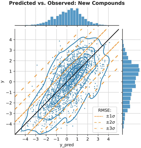
The factorization machine with the full feature set resulted in the lowest RMSE. To put the RMSE into context and assess how useful the models would be in practice, we plot the observed vs. expected toxicity values in Figures 6 and 7. The prediction of new chemicals is more difficult since there is more spread in the y-axis (Figure 7). We have also added diagonal lines to both figures, corresponding with ± 1, ±2, ±3 RMSE. The data is approximately log-normally distributed, so these correspond to ranges where 68.3, 95.4, and 99.7% of the true values occur for a given predicted value.

Figure 6. Scatter plot of model predictions and true values in the first validation setting: species and chemical interactions. We illustrate the expected deviation from the predicted values using diagonal bands, 68.3, 95.4, and 99.7% of observations, assuming a normal distribution based on the test RMSE.

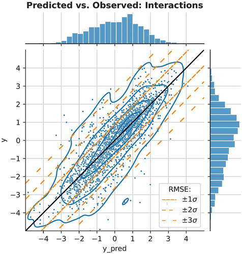
Figure 7. Scatter plot of model predictions and true values in the second validation setting: new chemicals. We illustrate the expected deviation from the predicted values using diagonal bands, 68.3, 95.4, and 99.7% of observations, assuming a normal distribution based on the test RMSE.

For the classification and labelling of chemicals, LC50 values are sometimes grouped into toxicity classes. Table 3 and Table 4 show the confusion matrices based on the predicted LC50 values of our proposed linear model within the first and the second validation setting. The models generally give the correct class within one magnitude of 10, but there are a few notable exceptions of extremely toxic chemicals being classified as non-toxic chemicals, and vice versa. Table S9 lists the precision and recall in each class based on the confusion matrix. It should be noted that most chemicals belong to the most toxic class (0,1], so the model optimized by the overall RMSE will be tilted towards accurate predictions in this class.

Table 3. Confusion matrix for toxicity class classification in the first setting: species and chemical interactions. Toxicity is expressed as LC50s in mg/L. Predicted class is listed the row, observed class in the column. Overall accuracy is 69%.

Predicted	(0, 1]	(1, 10]	(10, 100]	(100, 1000]	(1000, inf]
(0, 1]	20861	2861	605	118	14
(1, 10]	2928	7471	3428	454	30
(10, 100]	337	2024	5952	1745	245
(100, 1000]	72	106	627	1384	478
(1000, inf]	2	6	17	143	364

Table 4. Confusion matrix for toxicity class classification in the second setting: new chemicals. Toxicity is expressed as LC50s in mg/L. Predicted class is listed the row, observed class in the column. Overall accuracy is 54%.

Predicted	(0, 1]	(1, 10]	(10, 100]	(100, 1000]	(1000, inf]
(0, 1]	17064	3505	1204	222	26
(1, 10]	5531	6207	4040	910	140
(10, 100]	1248	2226	4017	1557	378
(100, 1000]	337	374	1016	914	413
(1000, inf]	20	156	352	241	174

Accuracy of machine learning models

Table 5 shows the performance of the baseline machine learning models and compares this to the proposed linear models and factorization machines. Factorization machines are the best model in the first setting. Support Vector machines are the best approach in the second setting, with other non-linear machine learning models achieving comparable results. This suggests chemical similarity could be a driving force of the predictions. The tree-based models, i.e. random forest and gradient boosting, do better than a standard ridge regression model, as could be expected, but are outperformed by the ridge regression that includes not only the global effect of species, chemical, and chemical fingerprints, but also the pairwise interactions between species and chemical fingerprints.

Table 5. Machine learning models accuracy in predicting interactions (validation setting 1) and new chemicals (validation setting 2).

Model	Implementation	RMSE (Interactions)	RMSE (New chemicals)
NULL		1.67	1.68
LM	scikit-learn	0.98	1.24
LM (interactions)	scikit-learn	0.93	1.18
RF	scikit-learn	1.01	1.20
XGB	xgboost	0.93	1.20
SVR	libsvm	0.93	1.16
NN	tensorflow	0.89	1.20
FM	xlearn	0.88	1.19
PERFECT		0.54^†	0.54^†

† Minimum achievable error calculated from residual variance.

Discussion

To manage the environmental risks associated with exposure of aquatic animal species to chemicals, chemical hazards need to be identified. However, this has become an increasingly challenging task due to the large number of chemicals being developed and brought to the market. It is practically impossible to perform experimental toxicity tests of all chemicals with a wide variety of animal species. Accurate models to predict chemical hazards for an as wide variety of animal species as possible, are therefore needed. With this in mind, we developed and applied a linear model based on ridge regression and factorization machines to predict the LC50 values associated with exposure to chemicals in a particular species and duration and compared the performance of this model to the performance of well-known machine learning methods. This work thus provides additional insights in the use and possibilities of these methodologies for toxicity predictions.

Model performance

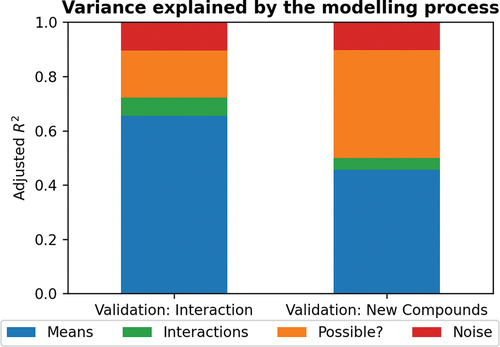
As a first step towards our objective, we trained a simple linear model. In developing the linear model, we found that the largest increase in performance results from learning the overall toxicity of a chemical (Table 1). For known chemicals, it is possible to include an indicator for the chemical which measures how toxic the chemical is on average over all species in training data. An indicator can also be included for the animal species, which will increase the model’s accuracy by learning how well a species, on average, survives when exposed to the chemicals in the experiments in the training data. This results in a surprisingly good accuracy but can be seen as trivial because the model predicts the same chemical toxicity for all species plus species survivability. For new chemicals, one must use the chemical features to predict the overall toxicity. The model is further improved by including an interaction between every species and chemical features, which allows every species to react differently to each chemical feature (Table 2). This is the most interesting aspect of pairwise models, and we were satisfied to find that such interactions exist in the data. This effectively means that species sensitivity is dependent on the type of chemical and underlines the need to have toxicity test results for multiple species in order to avoid under- or overestimation of the impact of exposure to a certain chemical in the aqueous environment. These findings are highlighted in Figure 8, which visualizes the percentage of explained variance using adjusted R².

Figure 8. The proportion of variance explained by first modelling the overall toxicity of chemicals and sensitivity of species, based on a regularized linear model on species indicators and chemical indicators/features (Means), and then including a pairwise interaction between every species and chemical features (Interaction) and the theoretical ceiling.

By extending the linear model using factorization machines, it is possible to fill the species-chemical LC50 matrix without features, even though the test set did not contain any (species-chemical) pair that is in the training data. The missing entries in the LC50 toxicity value matrix are filled by assuming that species or chemicals with similar observed toxicity outcomes respond similarly in the unobserved outcomes. This corresponds to the idea that some species (or chemicals) will react similarly to chemicals (or species) if they have a similar low-rank factorization. The same concept can be used for the interaction matrix of species and chemical features. The performance increased going from the linear model with interactions to the equivalent factorization machine model in the first setting (RMSE of 0.93 and 0.88, respectively), implying that transfer learning between species is possible. These findings suggest that predictive accuracy is based on three phenomena in the order of importance:

1. Global effects: some chemicals are more toxic on average over all species and some species have higher toxicity values on average over all chemicals they are tested on.

2. Global versus local model: the simplest form of transfer learning is to learn the same model for all species but converge to a species-specific model with sufficient data.

3. Transfer learning: sharing local models between species by assuming an underlying species similarity results in similar responses to either chemical or chemical features.

Machine learning methods with shallow architectures, i.e. methods with few computational layers, are in theory more flexible than traditional regression models through feature selection, including non-linear feature effects, and interactions between features. The tree-based machine learning models, such as Random Forest and XGboost, were indeed better than a simple linear model, but they were outperformed by the carefully regularized linear model with all pairwise interactions. This indicates that higher model complexity does not necessarily lead to better performances. Simple regression and tree-based models are not able to learn latent similarities, whereas the factorization machine and neural networks are.

The best performing models in the first validation setting predicting new species-chemical interactions, were the neural networks and the proposed factorization machine. Deep architectures, i.e. deep neural networks, might be able to learn a better model with more complex and unprocessed features, such as learning the relevant aspects of toxic chemicals from their molecular graph. However, this often comes at the cost of their interpretability [61], the risk of overfitting biological variability and/or noise, and manual labour needed to optimize their architecture. By including the latent similarities in the linear model with factorization machines, we were able to achieve similar performances to the neural network. In the second validation setting, the model performances of the different models were generally comparable, with the support vector machine having a slight edge over the other models. This again emphasizes that more complex models do not necessarily result in better performances.

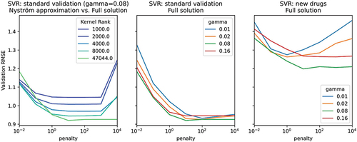
One drawback of machine learning methods is their sensitivity to the values of hyperparameters. Figure 9 for example shows how the SVR accuracy changes as a function of the kernel width and regularization penalty in the first training fold. Both parameters need to be jointly set at optimal values, which in turn depend on the validation setting that is considered. Typically, finding the optimal hyper-parameter values would be performed through an exhaustive grid search. However, considering it can take several hours to several days to fit a single SVR, such a grid search is impractical. Instead, the Nyström method for kernel approximation is often used to scale back the computing time, with the argument that the approximation is often good enough, but we found that the full solution was required in the first setting for the best results. In practice, the applicability of a machine learning method is highly dependent on the robustness of the method and the training time. Linear models, tree-based methods, and factorization machines have a definite advantage in this regard compared to SVRs, and NNs.

Figure 9. Visualization of the importance of hyperparameter tuning for the support vector regression (SVR). Both gamma and penalty hyperparameters need to be set carefully to their optimal values to achieve a competitive model. The full solution is required, since approximations that would speed up the model fitting time result in lower accuracy.

Besides applicability of the methodology in terms of the parameter tuning, the applicability domain of the model itself is also relevant, specifically for future applications. By the inclusion of a wide variety of species and chemicals, the predictions of the developed models are more generalizable and applicable to a relative wide range of organic chemicals. As in many other predictive models, inorganics including metals were not included in the model, as toxicity for these chemicals can be highly dependent on site-specific environmental properties such as pH. A quantitative evaluation allows one to assess whether the trained model is suited to predict toxicity of a particular chemical. A possible way of quantitatively determining the applicability domain is the Principal Component Analysis (PCA). Suvannang et al. [62] have already performed a PCA to determine the applicability domain of their model. With the PCA, they essentially compared the training dataset to the external test set, and concluded that the external test set fell within the boundaries of the chemical space of the training set. Their method, however, does not consider to what extent the test set is representative of the entire space of known chemicals. In practice, however, an even better way of determining the applicability domain would be to assess how well the training dataset falls within the entire chemical universe. This would enable a risk assessment to quantitatively determine whether the model is suited to predict toxicity for a particular chemical-species combination that is not present in the training or test data.

In addition, when developing models for regulatory purposes, the OECD principles need be followed [63]. The OECD principles dictate that an unambiguous algorithm and optionally a mechanistic interpretation are important for regulatory applications. Accordingly, our observation that a simple linear model based on learning low-rank interactions with factorization machines matches the accuracy of deep neural networks is valuable for follow-up studies. Particularly, as these relatively simple factorization machines also provide a direct interpretation into the underlying pattern of the predictions.

Future recommendations and applications

An important aspect of modelling biological responses is considering the biological and/or experimental variability. Repeated experiments with the same species, chemical and exposure duration can lead to different LC50 values. Quantifying the variability in the LC50 values in the dataset therefore provides an insight into the best possible model performance that can be achieved given the data. In the present study, we quantified the variability in the data by estimating the standard deviation among LC50 values measured in repeated experimental settings. We showed that the impact of biological and experimental variability could be substantial (Table 6). Such large variabilities are not uncommon in experimental toxicity testing, and comparable variations have been reported for other endpoints. For instance, for bioconcentration factors (BCF) in fish [64], and for No and Low Observed Adverse Effect Levels (N(L)OALSs) in rats and rabbits on developmental toxicity [65]. By quantifying the variability, we were able to show how the performances of the models compared to the best possible performance. Quantification of the variability in datasets should become common practice, as it facilitates the interpretation of the study outcomes, and helps comparing model performances between different studies. It should also help in avoiding overfitting of data by applying too complex model architectures to a modelling problem.

Table 6. The 95% confidence ranges of several LC50 values based on the approximate SD on ¹⁰log-scale of 0.54.

LC50 (mg/L)	Range (mg/L)	^10Log(LC50) (mg/L)	^10Log(range) (mg/L)
0.01	0.00083–0.12	−2.0	−3.1 – −0.92
0.5	0.042–6.0	−0.30	−1.4–0.78
2.5	0.21–30	0.40	−0.68–1.5
100	8.3–1200	2.0	0.92–3.1

A general challenge that is faced when applying machine learning methods is making sure that the quality of the data is sufficient. In this study, the ECOTOX database was consulted, which contains results reported from toxicity experiments. We did not extensively check whether the reported LC50 values in the ECOTOX database correspond to those reported in the individual studies, and besides the general data curation steps, described in the Methods section, we did not extensively evaluate the quality of individual studies using Klimisch scores [66] or CRED [67]. Furthermore, we did not consider a potential bias in the database towards results for more toxic substances. Substances that are expected to be more toxic are in general more likely to get tested. The chemicals included in the ECOTOX database may therefore represent a subset of relatively toxic chemicals and it is not clear whether this bias directly or indirectly affected the models developed.

The models implemented in the current study were trained using species indicators, but no species features. In principle, one could potentially improve the model performance by including species features during training. Such features may, for example, be the species body weight or size, or the average life expectancy. However, more complex features may also be used such as parts of the genome. Further research should be conducted to investigate whether the inclusion of species features improves the model performances.

Conclusion

The need to obtain toxicity assessments for multiple chemicals and for multiple species, whilst considering different exposure durations, costs and ethical considerations, requires the adoption of predictive models to replace animal testing. Generalizing to multiple species and chemicals is possible with large and sparse data sets, such as the ECOTOX database. Recommender systems have a long history of research on similar problems. This inspired our approach of modelling (species, chemical)-interactions using a simple linear model based on ridge regression with pairwise interactions and learning low-rank pairwise interactions with factorization machines. We showed that the model can match the accuracy of complex ML methods and gives a direct interpretation into the underlying pattern of the predictions. This insight can be used to further develop effective methods and applied to relevant problems that need to predict the toxicity of a chemical over multiple species.

Acknowledgements

The authors kindly acknowledge the critical reading of a previous version of the manuscript by Xiaoheng Huang.

Disclosure statement

No potential conflict of interest was reported by the author(s).

Supplementary data

Supplemental data for this article can be accessed at: https://doi.org/10.1080/1062936X.2023.2254225

Additional information

Funding

This research was supported by the Strategic Research Program (SPR) of RIVM by means of the MIGRATION project. Funding was also received from the European Union’s Horizon 2020 research and innovation programme under grant agreement Nº 101036449 (PROMISCES).

References

- C. van Leeuwen and T. Vermeire, Risk Assessment of Chemicals: An Introduction, Vol. 94, Springer, Dordrecht, The Netherlands, 2007. doi:10.1007/978-1-4020-6102-8.
- P.C. Thomas, P. Bicherel, and F.J. Bauer, How in silico and QSAR approaches can increase confidence in environmental hazard and risk assessment, Integr. Environ. Assess. Manage. 15 (2019), pp. 40–50. doi:10.1002/ieam.4108.
- R.T. Wright, K. Fay, A. Kennedy, K. Mayo-Bean, M. Moran-Bruce, W. Meylan, P. Ranslow, M. Lock, J.V. Nabholz, J. Von Runnen, C.L. M, and J. Tunkel, ECOlogical Structure-Activity Relationship Model (ECOSAR) Class Program, U.S. Environmental Protection Agency, Washington, DC, U.S., 2022.
- G. Idakwo, J. Luttrell, M. Chen, H. Hong, Z. Zhou, P. Gong, and C. Zhang, A review on machine learning methods for in silico toxicity prediction, J. Environ. Sci. Health C 36 (2018), pp. 169–191. doi:10.1080/10590501.2018.1537118.
- W. Tang, J. Chen, Z. Wang, H. Xie, and H. Hong, Deep learning for predicting toxicity of chemicals: A mini review, J. Environ. Sci. Health C 36 (2018), pp. 252–271. doi:10.1080/10590501.2018.1537563.
- A.O. Basile, A. Yahi, and N.P. Tatonetti, Artificial intelligence for drug toxicity and safety, Trends Pharmacol. Sci. 40 (2019), pp. 624–635. doi:10.1016/j.tips.2019.07.005.
- H.L. Ciallella and H. Zhu, Advancing computational toxicology in the big data era by artificial intelligence: Data-driven and mechanism-driven modeling for chemical toxicity, Chem. Res. Toxicol. 32 (2019), pp. 536–547. doi:10.1021/acs.chemrestox.8b00393.
- Z. Lin and W.C. Chou, Machine learning and artificial intelligence in toxicological sciences, Toxicol. Sci. 189 (2022), pp. 7–19. doi:10.1093/toxsci/kfac075.
- N.C. Kleinstreuer, A. Karmaus, K. Mansouri, D.G. Allen, J.M. Fitzpatrick, and G. Patlewicz, Predictive models for acute oral systemic toxicity: A workshop to bridge the gap from research to regulation, Comput. Toxicol. 8 (2018), pp. 21–24. doi:10.1016/j.comtox.2018.08.002.
- R. Huang, M. Xia, D.-T. Nguyen, T. Zhao, S. Sakamuru, J. Zhao, S.A. Shahane, A. Rossoshek, and A. Simeonov, Tox21 challenge to build predictive models of nuclear receptor and stress response pathways as mediated by exposure to environmental chemicals and drugs, Front. Environ. Sci. 3 (2016). doi:10.3389/fenvs.2015.00085.
- A. Mayr, G. Klambauer, T. Unterthiner, and S. Hochreiter, DeepTox: Toxicity prediction using deep learning, Front. Environ. Sci. 3 (2016). doi:10.3389/fenvs.2015.00080.
- Y. Xu, J. Pei, and L. Lai, Deep learning based regression and multiclass models for acute oral toxicity prediction with automatic chemical feature extraction, J. Chem. Inf. Model. 57 (2017), pp. 2672–2685. doi:10.1021/acs.jcim.7b00244.
- S. Sosnin, D. Karlov, I.V. Tetko, and M.V. Fedorov, Comparative study of multitask toxicity modeling on a broad chemical space, J. Chem. Inf. Model. 59 (2019), pp. 1062–1072. doi:10.1021/acs.jcim.8b00685.
- A. Karim, V. Riahi, A. Mishra, M.A.H. Newton, A. Dehzangi, T. Balle, and A. Sattar, Quantitative toxicity prediction via meta ensembling of multitask deep learning models, ACS Omega 6 (2021), pp. 12306–12317. doi:10.1021/acsomega.1c01247.
- S. Jain, V.B. Siramshetty, V.M. Alves, E.N. Muratov, N. Kleinstreuer, A. Tropsha, M.C. Nicklaus, A. Simeonov, and A.V. Zakharov, Large-scale modeling of multispecies acute toxicity end points using consensus of multitask deep learning methods, J. Chem. Inf. Model. 61 (2021), pp. 653–663. doi:10.1021/acs.jcim.0c01164.
- G.E. Dahl, N. Jaitly, and R. Salakhutdinov, Multi-task neural networks for qsar predictions, ArXiv preprint ArXiv:1406.1231 2014.
- K. Wu and G.W. Wei, Quantitative toxicity prediction using topology based multitask deep neural networks, J. Chem. Inf. Model. 58 (2018), pp. 520–531. doi:10.1021/acs.jcim.7b00558.
- S. Gupta, N. Basant, and K.P. Singh, Predicting aquatic toxicities of benzene derivatives in multiple test species using local, global and interspecies QSTR modeling approaches, RSC Adv. 5 (2015), pp. 71153–71163. doi:10.1039/C5RA12825K.
- L. Sun, C. Zhang, Y. Chen, X. Li, S. Zhuang, W. Li, G. Liu, P.W. Lee, and Y. Tang, In silico prediction of chemical aquatic toxicity with chemical category approaches and substructural alerts, Toxicol. Res. 4 (2015), pp. 452–463. doi:10.1039/C4TX00174E.
- N. Basant, S. Gupta, and K.P. Singh, Modeling the toxicity of chemical pesticides in multiple test species using local and global QSTR approaches, Toxicol. Res. 5 (2016), pp. 340–353. doi:10.1039/C5TX00321K.
- F. Li, D. Fan, H. Wang, H. Yang, W. Li, Y. Tang, and G. Liu, In silico prediction of pesticide aquatic toxicity with chemical category approaches, Toxicol. Res. 6 (2017), pp. 831–842. doi:10.1039/C7TX00144D.
- B.A. Tuulaikhuu, H. Guasch, and E. Garcia-Berthou, Examining predictors of chemical toxicity in freshwater fish using the random forest technique, Environ. Sci. Pollut. Res. Int. 24 (2017), pp. 10172–10181. doi:10.1007/s11356-017-8667-4.
- T.Y. Sheffield and R.S. Judson, Ensemble QSAR modeling to predict multispecies fish toxicity lethal concentrations and points of departure, Environ. Sci. Technol. 53 (2019), pp. 12793–12802. doi:10.1021/acs.est.9b03957.
- X. Yu and Q. Zeng, Random forest algorithm-based classification model of pesticide aquatic toxicity to fishes, Aquat. Toxicol. 251 (2022), pp. 106265. doi:10.1016/j.aquatox.2022.106265.
- J. Wu, S. D’Ambrosi, L. Ammann, J. Stadnicka-Michalak, K. Schirmer, and M. Baity-Jesi, Predicting chemical hazard across taxa through machine learning, Environ. Int. 163 (2022), pp. 107184. doi:10.1016/j.envint.2022.107184.
- R. Caruana, Multitask learning, Mach. Learn. 28 (1997), pp. 41–75. doi:10.1023/A:1007379606734.
- K. Weiss, T.M. Khoshgoftaar, and D. Wang, A survey of transfer learning, J. Big Data 3 (2016). doi:10.1186/s40537-016-0043-6.
- J. Jiang, R. Wang, M. Wang, K. Gao, D.D. Nguyen, and G.W. Wei, Boosting tree-assisted multitask deep learning for small scientific datasets, J. Chem. Inf. Model. 60 (2020), pp. 1235–1244. doi:10.1021/acs.jcim.9b01184.
- D. Spurgeon, E. Lahive, A. Robinson, S. Short, and P. Kille, Species sensitivity to toxic substances: Evolution, ecology and applications, Front. Environ. Sci. 8 (2020). doi:10.3389/fenvs.2020.588380.
- D.H. Park, H.K. Kim, I.Y. Choi, and J.K. Kim, A literature review and classification of recommender systems research, Expert Syst. Appl. 39 (2012), pp. 10059–10072. doi:10.1016/j.eswa.2012.02.038.
- J. Lu, D. Wu, M. Mao, W. Wang, and G. Zhang, Recommender system application developments: A survey, Dec. Supp. Syst 74 (2015), pp. 12–32. doi:10.1016/j.dss.2015.03.008.
- J.B. Schafer, D. Frankowski, J. Herlocker, and S. Sen, Collaborative filtering recommender systems, in The Adaptive Web: Methods and Strategies of Web Personalization, P. Brusilovsky, A. Kobsa, and W. Nejdl, eds., Springer Berlin Heidelberg, Berlin, Heidelberg, 2007, pp. 291–324. doi:10.1007/978-3-540-72079-9_9.
- M.J. Pazzani and D. Billsus, Content-based recommendation systems, in The Adaptive Web: Methods and Strategies of Web Personalization, P. Brusilovsky, A. Kobsa, and W. Nejdl, eds., Springer Berlin Heidelberg, Berlin, Heidelberg, 2007, pp. 325–341. doi:10.1007/978-3-540-72079-9_10.
- Y. Koren, R. Bell, and C. Volinsky, Matrix factorization techniques for recommender systems, Computer 42 (2009), pp. 30–37. doi:10.1109/MC.2009.263.
- S. Rendle, L. Zhang, and Y. Koren, On the difficulty of evaluating baselines: A study on recommender systems, Arxiv preprint ArXiv:1905.01395 2019.
- J. Basilico and T. Hofmann, Unifying collaborative and content-based filtering, Proceedings of the twenty-first international conference on Machine learning. doi:10.1145/1015330.1015394.
- T. Pahikkala, A. Airola, S. Pietila, S. Shakyawar, A. Szwajda, J. Tang, and T. Aittokallio, Toward more realistic drug-target interaction predictions, Brief. Bioinf. 16 (2015), pp. 325–337. doi:10.1093/bib/bbu010.
- R. Chen, X. Liu, S. Jin, J. Lin, and J. Liu, Machine learning for drug-target interaction prediction, Molecules 23 (2018), pp. 2208. doi:10.3390/molecules23092208.
- M. Bagherian, E. Sabeti, K. Wang, M.A. Sartor, Z. Nikolovska-Coleska, and K. Najarian, Machine learning approaches and databases for prediction of drug-target interaction: A survey paper, Brief. Bioinf. 22 (2021), pp. 247–269. doi:10.1093/bib/bbz157.
- M. Wen, Z. Zhang, S. Niu, H. Sha, R. Yang, Y. Yun, and H. Lu, Deep-learning-baseddrug-target interaction prediction, J. Proteome Res. 16 (2017), pp. 1401–1409. doi:10.1021/acs.jproteome.6b00618.
- G.J.P. van Westen, J.K. Wegner, A.P. Ijzerman, H.W.T. van Vlijmen, and A. Bender, Proteochemometric modeling as a tool to design selective compounds and for extrapolating to novel targets, MedChemComm 2 (2011), pp. 16–30. doi:10.1039/C0MD00165A.
- D. Erhan, J. L’Heureux P, S.Y. Yue, and Y. Bengio, Collaborative filtering on a family of biological targets, J. Chem. Inf. Model. 46 (2006), pp. 626–635. doi:10.1021/ci050367t.
- J. Gao, D. Che, V.W. Zheng, R. Zhu, and Q. Liu, Integrated QSAR study for inhibitors of hedgehog signal pathway against multiple cell lines: A collaborative filtering method, BMC Bioinf. 13 (2012), pp. 186. doi:10.1186/1471-2105-13-186.
- M. Ammad-Ud-Din, E. Georgii, M. Gonen, T. Laitinen, O. Kallioniemi, K. Wennerberg, A. Poso, and S. Kaski, Integrative and personalized QSAR analysis in cancer by kernelized Bayesian matrix factorization, J. Chem. Inf. Model. 54 (2014), pp. 2347–2359. doi:10.1021/ci500152b.
- D.-S. Huang, K.-H. Jo, and X.-L. Zhang (eds.), Using Hybrid Similarity-Based Collaborative Filtering Method for Compound Activity Prediction, Springer International Publishing, 2018.
- J.H. Olker, C.M. Elonen, A. Pilli, A. Anderson, B. Kinziger, S. Erickson, M. Skopinski, A. Pomplun, C.A. LaLone, C.L. Russom, and D. Hoff, The ECOTOXicology knowledgebase: A curated database of ecologically relevant toxicity tests to support environmental research and risk assessment, Environ. Toxicol. Chem. 41 (2022), pp. 1520–1539. doi:10.1002/etc.5324.
- E.s.N.C.f.C. Toxicology, Chemistry Dashboard Data: DSSTox QSAR Ready File, The United States Environmental Protection Agency’s Center for Computational Toxicology and Exposure, U.S. Environmental Protection Agency, Washington, DC, U.S., 2018.
- K. Mansouri, C.M. Grulke, R.S. Judson, and A.J. Williams, OPERA models for predicting physicochemical properties and environmental fate endpoints, J. Cheminform. 10 (2018), pp. 10. doi:10.1186/s13321-018-0263-1.
- G. Landrum, P. Tosco, and B. Kelley, Ric, sriniker, gedeck, R. Vianello, D. Cosgrove, N. Schneider, E. Kawashima, N. Dan, A. Dalke, G. Jones, B. Cole, M. Swain, S. Turk, A. Savelyev, A. Vaucher, M. Wójcikowski, I. Take, D. Probst, K. Ujihara, V.F. Scalfani, G. Godin, A. Pahl, F. Berenger, J.L. Varjo, and D. Gavid, rdkit, 2022.
- G.L. Hickey, P.S. Craig, R. Luttik, and D. de Zwart, On the quantification of intertest variability in ecotoxicity data with application to species sensitivity distributions, Environ. Toxicol. Chem. 31 (2012), pp. 1903–1910. doi:10.1002/etc.1891.
- G. Varoquaux, L. Buitinck, G. Louppe, O. Grisel, F. Pedregosa, and A. Mueller, Scikit-learn, GetMobile: Mobile Comput. Comm. 19 (2015), pp. 29–33. doi:10.1145/2786984.2786995.
- Y. Juan, Y. Zhuang, W.-S. Chin, and C.-J. Lin, Field-aware factorization machines for CTR prediction, Proceedings of the 10th ACM Conference on Recommender Systems Association for Computing Machinery, Boston, Massachusetts, USA, 2016.
- L. Breiman, Random forests, Mach. Learn. 45 (2001), pp. 5–32. doi:10.1023/A:1010933404324.
- J.H. Friedman, Greedy function approximation: A gradient boosting machine, Ann. Stat. 29 (2001). doi:10.1214/aos/1013203451.
- T. Chen, T. He, and M. Benesty, Xgboost: Extreme gradient boosting. R package version 0.4-2, 2015.
- C. Williams and M. Seeger, Using the Nyström method to speed up kernel machines, 2000.
- R.E. Fan, K.-W. Chang, C.-J. Hsieh, X.-R. Wang, and C.-J. Lin, LIBLINEAR: A library for large linear classification, J. Mach. Learn. Res. 9 (2008), pp. 1871–1874.
- C.-C. Chang and C.-J. Lin, Libsvm: A library for support vector machines, ACM Trans. Intell. Syst.Technol. 2 (2011), pp. 1–27. doi:10.1145/1961189.1961199.
- W. Samek, G. Montavon, S. Lapuschkin, C.J. Anders, and K.-R. Muller, Explaining deep neural networks and beyond: A review of methods and applications, Proceed. IEEE 109 (2021), pp. 247–278. doi:10.1109/JPROC.2021.3060483.
- G.E. Dahl, T.N. Sainath, and G.E. Hinton, Improving deep neural networks for LVCSR using rectified linear units and dropout, 2013 IEEE International Conference on Acoustics, Speech and Signal Processing, IEEGeorge, IEEE, Vancouver, BC, Canada.
- J. Hemmerich and G.F. Ecker, In silico toxicology: From structure-activity relationships towards deep learning and adverse outcome pathways, Interdiscip. Rev. Comput. Mol. Sci. 10 (2020), pp. e1475. doi:10.1002/wcms.1475.
- N. Suvannang, L. Preeyanon, A.A. Malik, N. Schaduangrat, W. Shoombuatong, A. Worachartcheewan, T. Tantimongcolwat, and C. Nantasenamat, Probing the origin of estrogen receptor alpha inhibition via large-scale QSAR study, RSC Adv. 8 (2018), pp. 11344–11356. doi:10.1039/C7RA10979B.
- O.F.E.C.-o.a.D. (OECD), The report from the expert group on (quantitative) structure-activity relationships [(q)sars] on the principles for the validation of (Q)sars, 2004.
- P.N.H. Wassenaar, E.M.J. Verbruggen, E. Cieraad, W. Peijnenburg, and M.G. Vijver, Variability in fish bioconcentration factors: Influences of study design and consequences for regulation, Chemosphere 239 (2020), pp. 124731. doi:10.1016/j.chemosphere.2019.124731.
- H.M. Braakhuis, P.T. Theunissen, W. Slob, E. Rorije, and A.H. Piersma, Testing developmental toxicity in a second species: Are the differences due to species or replication error? Regul. Toxicol. Pharmacol. 107 (2019), pp. 104410. doi:10.1016/j.yrtph.2019.104410.
- H.J. Klimisch, M. Andreae, and U. Tillmann, A systematic approach for evaluating the quality of experimental toxicological and ecotoxicological data, Regul. Toxicol. Pharmacol. 25 (1997), pp. 1–5. doi:10.1006/rtph.1996.1076.
- C.T. Moermond, R. Kase, M. Korkaric, and M. Agerstrand, CRED: Criteria for reporting and evaluating ecotoxicity data, Environ. Toxicol. Chem. 35 (2016), pp. 1297–1309. doi:10.1002/etc.3259.