Different approaches for the solution of a backward heat conduction problem

Abstract

This work presents a comparison of three different techniques to solve the inverse heat conduction problem involving the estimation of the unknown initial condition for a one-dimensional slab, whose solution is obtained through minimization of a known functional form. The following techniques are employed to solve the inverse problem: the conjugate gradient method with the adjoint equation, regularized solution using a quasi-Newton method, and regularized solution via genetic algorithm (GA) method. For the first one, a general form to compute the gradient of the functional form (considering the time and space domains) is presented, and for the GA method a new genetic operator named epidemical is applied.

Keywords:

• Inverse problem
• Heat conduction
• Alifanov's iterative regularization method
• Regularized solutions
• Epidemical genetic algorithms

1 Introduction

Forward heat conduction problems are focused on determination of the temperature field of the medium, when the boundary and initial conditions, heat source–sink terms (if any), and the physical properties of the material are known. On the other hand, an inverse heat conduction problem is concerned with the estimation of such quantities (boundary or initial conditions, source–sink terms, physical properties) from the temperature and/or heat flux measurements.

Inverse problems as well as their solving tools certainly have been one of the fastest growing areas in various application fields. Mathematically they are classified as ill-posed problems. A problem is considered well-posed if the following requirements are satisfied: the solution of the problem exists, it is unique and stable with respect to the input data [1]. The existence of a solution for an inverse heat transfer problem can be assured based on physical reasoning, but the requirement of uniqueness can only be formally proved for some special cases. Also, the inverse problem solution is generally unstable. Therefore, small perturbations in the input data, like random errors inherent to the measurements used in the analysis, can cause large oscillations on the solution.

In accordance with the type of information that is being sought in the solution procedure, the inverse heat conduction problems may be classified as [2]

	Backward or retrospective problem, when initial conditions are to be found;
	Coefficient inverse problem, when a parameter in governing equation is to be found;
	Boundary inverse problem, when some missing information at the boundary of a domain is to be found.

Another means of sorting is based on the statistical nature of the method employed for solving an inverse problem [3]

	Deterministic;
	Stochastic.

Based on the sorting presented above, the techniques considered in this work present a comparison of both deterministic and stochastic methods, besides the variational method, as applied to solve the backward (or retrospective) problem of estimating the unknown initial condition of a one-dimensional slab. For the reconstruction treated here, the ill-posed problem is presented as a well-posed functional form, whose solution is obtained through an optimization problem.

Such an inverse problem has been previously addressed in the literature by using regularization approaches [4–6] and the conjugate gradient method with the adjoint equation or Alifanov's iterative regularization method [7]. Solution techniques utilized here include the conjugate gradient method with the adjoint equation [8–10], regularized solution using a quasi-Newton method [5,6], and regularized solution through the genetic algorithm (GA) method [11–14]. This last method has been applied to solve other classes of inverse problems, such as the magnetotelluric inversion [15,16], and damage identification [17].

The conjugate gradient method with the adjoint equation is an iterative method, in which the regularization is implicitly built in the computational procedure. The quasi-Newton method belongs to the class of the generalized least square methods, which, in this work, will be related to regularization by maximum entropy principle [5,18,19]. The GA is applied to optimization problems trying to minimize the deviation between the behavior predicted by a candidate model and that actually observed, the measured data. Such deviation will be represented by an objective function which is associated with Tikhonov's regularization [20].

2 The Direct Problem

The direct (forward) problem consists of a transient heat conduction problem in a slab with adiabatic boundary condition and initially at a temperature denoted by f (x).

The mathematical formulation of this problem is given by the following heat equation:

where T(x,t) (temperature), f (x) (initial condition), x (spatial variable), and t (time variable), are nondimensional quantities. The solution of the direct problem for x ∈ (0,1) and t > 0 for a given initial condition f (x) is given by

where X(β _m,x) are the eigenfunctions associated to the problem, and β_m and N(β_m ) are, respectively, the corresponding eigenvalues and norms [21]. The function f is assumed to be bounded satisfying Dirichlet's conditions in the interval [0,1] [22]. The eigenfunctions, eigenvalues, and the norm for the problem defined by Eqs. (1)–(3) can be precisely expressed as

Assuming is the final time, this solution could be expressed in a discrete form

where I is the total subdivision number of the interval of interest (integration domain), and the series (4) has been truncated considering M _max terms. This solution could also be expressed in a compact form

where

Hence, the temperature profile T(x,τ) can be determined by solving the matrix system

where τ is the final time.

3 The Inverse Problem

As mentioned before, a transient heat conduction problem in a slab is considered, with both boundaries kept insulated. Here, the goal is to estimate the unknown initial temperature distribution f, from the knowledge of the measured temperatures T at the time t = τ > 0, for a finite number of different locations in the domain.

The solution of this inverse heat conduction problem employing the techniques considered here, is based on the minimization of a functional form given by

where is the experimental data (t = τ > 0), T ^Mod is the temperature obtained using the initial condition recovered (f_ξ ), Ω (f) denotes the regularization term, ξ is the regularization parameter, and ||·||₂ is the 2-norm.

3.1 Variational Method – Alifanov's Approach

The variational method, also known as conjugate gradient method with the adjoint equation or Alifanov's approach, involves the following basic steps: (i) the solution of forward problem; (ii) the solution of sensitivity problem; (iii) the solution of adjoint problem and the gradient equation; (iv) the conjugate gradient method of minimization; and (v) the discrepancy principle for stopping criteria. A brief description of basic procedures involved in each of these steps (see also [23]) is presented.

3.1.1 The Forward Problem Solution

The mathematical solution for the forward problem, Eqs. (1)–(3), is given by the Eq. (4) or (8), when the initial temperature distribution f (x) is known.

3.1.2 The Sensitivity Problem

The sensitivity problem is obtained assuming that the initial temperature distribution f (x) undergoes an increment ▵f (x), and the temperature T(x,t) changes by an amount ▵T(x,t). Therefore, in order to obtain the sensitivity problem that satisfies the function ▵T(x,t), T(x,t) is replaced by T(x,t) + ▵T(x,t) and f (x) by f (x) + ▵f (x) in the direct problem given by the Eqs. (1)–(3), subtracting from the original problem. The sensitivity problem, is then, obtained

3.1.3 The Adjoint Problem and the Gradient Equation

Since the inverse problem does not satisfy the requirements of existence and uniqueness, it is to be solved as an optimization problem requiring that the unknown function f (x) should minimize the functional form J [f (x)] defined by Eq. (9), when ξ = 0 is considered:

where τ is the final time, M is the number of sensors, and T_m (t) and are the dimensionless computed and measured temperatures, respectively, at each sensor location as a function of time.

The adjoint problem is obtained by introducing a new function λ (x,t), called the Lagrange multiplier [8]. Equation (1) is multiplied by the Lagrange multiplier (or adjoint function) λ (x,t), integrating the resulting expression over time and space domain and adding the result to the functional given by (13). This mathematical manipulation leads to the adjoint problem

and an integral term expressed as

To compute the gradient of the functional form, consider the limit when t → 0 in the Eq. (17)

On the other hand, in the space of integrable square functions, by definition, the following relation holds [8,10,24]

where J′(x) is the gradient of the functional J(x).

Considering the limit when t → 0 in the Eq. (19)

Therefore,

A comparison of Eqs. (18) and (20) reveals that the gradient of the functional, J′(x), is given by

3.1.4 The Conjugate Gradient Method of Optimization

The unknown function f (x) can be determined by a process based on the minimization of the functional J [f (x)]. If the conjugated gradient method is used [8,10] the recurrence equation for the determination of f (x) can be given by

where the β^k is the step size given by

and P^k , the direction of descent, given by

where γ^k is the conjugate coefficient given by

3.1.5 The Stopping Criterion

If the problem contains no measurement errors, one can use the customary stopping criteria

where ϵ* is a small specified number. However, in practical applications, measurement errors are always present; therefore, the discrepancy principle as described below should be used to establish the stopping criteria [8,9].

Let the standard deviation σ of the measurement errors be the same for all sensors and measurements, that is,

Introducing this result into Eq. (13) we obtain

Then the discrepancy principle for the stopping criteria is taken as

3.1.6 Inverse Analysis Algorithm

The computational procedure is summarized in the following algorithm:

• Step 1 Choose an initial guess f ⁰(x) – for example, f ⁰(x) = constant.

• Step 2 Solve the direct problem given by Eqs. (1)–(3) to obtain T(x,t).

• Step 3 Solve the adjoint problem (14)–(16), to obtain λ (x,t).

• Step 4 Knowing λ (x,t), compute the gradient function J′(f) from Eq. (21).

• Step 5 Compute the conjugate coefficient γ^k from Eq. (25).

• Step 6 Compute the direction of descent P^k (x) from Eq. (24).

• Step 7 Setting Δ f (x) = P^k (x) [10], solve the sensitivity problem (10)–(12) to obtain Δ T(x,t).

• Step 8 Compute the step size β^k from Eq. (23).

• Step 9 Compute f^{k + 1}(x) from Eq. (22).

• Step 10 Test if the stopping criteria, Eq. (29), is satisfied. If not, go to Step 2.

3.2 Regularized Deterministic Method – Quasi-Newton Scheme

The application of this technique is characterized by the minimization of the objective function given by the Eq. (9). Just as in the minimum norm least-squares, it can guarantee the existence and uniqueness, but this solution can be unstable in the presence of noise in the experimental data, thus requiring the use of some regularization technique [20]. The regularized solution is obtained by choosing the function f_ξ (x) that minimizes the following functional form:

where T ^Exp is the experimental data (t = τ > 0), T ^Mod is the temperature obtained using a given initial condition, Ω (f) denotes the regularization term, and ξ is the regularization parameter.

The regularization parameter ξ is chosen numerically, through a posteriori parameter choice rule, assuming that the statistics of the measurement errors are known. These numerical experiments are based on the Morozov's discrepancy principle [25,26], where the optimum regularization parameter ξ^⋆ must be chosen such that .

The regularization technique applied in this approach is based on the maximum entropy principle [18,19]. In this way, the objective function is given by

The minimization of the objective function given by the Eq. (31), subject to simple bounds on f, is solved using a first-order optimization from the NAG Fortran library [27]. This routine is designed to minimize an arbitrary smooth function subject to constraints (simple bounds, linear and nonlinear constraints), using a sequential programming method. For the nth iteration, the calculation proceeds as follows:

1. Solve the direct problem for f ⁿ, and compute the objective function .

2. Compute the gradient using finite differences.

3. Compute a positive-definite quasi-Newton approximation to the Hessian H ⁿ:

   where

4. Compute the search direction d ⁿ as a solution of the following quadratic programming subproblem :

5. Set f ^{n + 1} = f ⁿ + βⁿ d ⁿ , where the step length β ⁿ minimizes .

6. Test the convergence; stop or return to Step 1.

3.3 Regularized Stochastic Method – Genetic Algorithm

Genetic algorithms are essentially optimization algorithms whose solutions evolve somehow from the science of genetics and the processes of natural selection – the Darwinian principle. They differ from more conventional optimization techniques since they work on whole populations of encoded solutions, and each possible solution is encoded as a gene. Differences between conventional search techniques and the GAs can be summarized as follows [12]:

	The GA works with a coding for the parameter set, not the parameters themselves;
	The GA searches from a population of points, not a single point;
	The GA uses the objective function's information, not derivatives or other auxiliary knowledge;
	The GA uses probabilistic transition rules, not deterministic rules.

The most important phases in GAs standard are selection (competition), reproduction, mutation and fitness evaluation. Selection is an operation used to decide which individuals to use for reproduction and mutation in order to produce new search points. Reproduction or crossover is the process by which the genetic material from two parent individuals is combined to obtain one or more offsprings. Mutation is normally applied to one individual in order to produce a new version of it where some of the original genetic material has been randomly changed. Fitness evaluation is the step in which the quality of an individual is assessed.

The application of GA method to solve the problem of estimation of the initial temperature is also a minimization problem, as well as the quasi-Newton method, where the regularized functional form employed is the same given by Eq. (30). However, the regularization technique used in this case is the Tikhonov regularization of order 0 and 1: where k=0 or 1 representing the derivative (continuous case) or difference (discrete case) operator. Introducing this term in the regularized functional form, the fitness or objective function is defined by

In this implementation, the algorithm operates on a fixed-sized population which is randomly generated initially. The members of this population are fixed-length and real-valued strings that encode the variable which the algorithm is trying to optimize (f_ξ ). Next, a pseudocode of the GA employed is presented, where a new evolutionary operator is applied:

Genetic_algorithm

 Define and initialize the evolutionary parameters;

 t ≔ 0;

 Generate a random population Pop(t);

 Calculate the fitness J(f_ξ )of each individual in Pop(t);

 While (condition)

  t ≔ t + 1;

  Select a pair of parents from Pop(t − 1);

  Cross over the pair of parents selected;

  Mutate the new string X generated;

  Insert the individual X in the worst location of Pop(t − 1);

  Calculate the fitness of the individual X;

  X*(t) ≔ Best[Pop(t)];

  If(X*(t) = X*(t − 1))then

   cont_epidemic ≔ cont_epidemic + 1;

   If (cont_epidemic > limit) then

    Apply Epidemical on Pop(t);

   End_If

  End_If

 End_While

End

Some different evolutionary operators have been tested in this specific inverse problem, and some of them have presented better results than others. Among the operators tested, beyond those presented below, one can cite the roulette selection operator [12], the sphere [13] and blend [28] crossover operators, and the uniform mutation operator [13]. Following, the evolutionary operators actually employed in this work are presented.

	Tournament Selection [14] bigger ≔ rand; smaller ≔ rand; val ≔ 0.75; if (rand < val) then  position ≔ bigger; else  position ≔ smaller; endif where rand is a random number from [0,1) with uniform distribution, bigger is the best fitness individual and smaller is the worst fitness individual.
	Geometrical Crossover [13] This crossover operator breeds only one offspring from two parents. From the parents xi and yi the offspring is represented by where μ is a number between [0, 1]. A typical value is μ = 1/2, where the same weight is given to both parents.
	Nonuniform Mutation [13] This mutation operator is defined by such as where rand is a random number from [0,1) with uniform distribution, T is the maximal generation number, t is the generation number, and b is a system parameter determining the degree of non-uniformity.
	Epidemical Strategy Beyond standard genetic operators described before, a new operator called epidemical has been used. This operator is activated when a specific number of generations is reached without improvement of the best individual. When it is activated, all the individuals are affected by a plague, and only those that have the best fit (e.g., first 2% with the best fit in the population) survive. The remaining die and their place is occupied by new individuals with new genetic variability, such as immigrants arriving, to continue the work that was done before by others.

This operator has two free parameters that need to be found. One of them determines the instant that the strategy will be activated; i.e., the generation number without improvement of the best individual fit that will be considered. Another parameter to be determined is the amount of individuals that will be kept in the population, the amount that will survive the plague.

At present work, the new individuals have been generated randomly, just as the initial population, and 98% of the population have been substituted, preserving 2% of the old population.

4 Numerical Results

In this article we have described three different techniques to solve the backward heat conduction problem involving the estimation of the unknown initial condition for a one-dimensional slab, and these techniques have been tested for two different initial temperature profiles:

1. Triangular test function:

2. Semitriangular test function:

The experimental data (measured temperatures at a time τ > 0) are obtained from the exact solution of the direct problem (noiseless data) or by adding a random perturbation error to the exact solution of the direct problem (noisy data)

where σ is the standard deviation of the errors and is a random variable taken from a normal distribution such that ormal(0;1). For numerical purposes, it has been adopted τ = 0.01 s and σ = 0.05 and the spatial grid consisting of 101 points (M = 101).

All the three techniques have been tested considering the two different test functions and the two different data type (noiseless and noisy data). It should be noted that when noisy data is considered, all the techniques consider the application of regularization, either by regularizated functionals (quasi-Newton and GA) or by regularization built in the computational procedure of the conjugate gradient method utilizing the adjoint equation (Alifanov's approach).

In order to determine which of the techniques provide a better estimation of the initial condition, the same experimental profile of temperature at time τ has been used in all simulations; i.e., the same random error was applied to all simulations. In the same way, the error between the approximated (or calculated) solution f_ξ and the exact solution f _exact of the inverse problem has been employed to compare all the methods tested. In this way, the error is defined by

and its values are presented in Tables I and II referring to noiseless and noisy data, respectively.

TABLE I Error values for noiseless data – Eq. (40)

Estimation errors with noiseless data
Method employed	Triangular function	Semitriangular function
Alifanov	0.00756	0.01741
Quasi-Newton	0.02209	0.10155
Genetic algorithm	2.01913	5.89825
Genetic algorithm*	2.36247	5.57705

TABLE II Error values for noisy data – Eq. (40)

Estimation errors with noisy data
Method employed	Triangular function	Semitriangular function
Alifanov	0.12213	0.13708
Quasi-Newton	0.15272	0.26307
Genetic algorithm	0.10623	0.15315
Genetic algorithm*	0.15778	0.23324
Genetic algorithm†	0.11485	0.77282

4.1 Noiseless Data

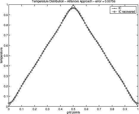
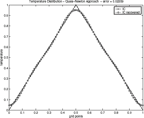
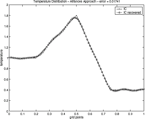
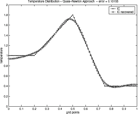
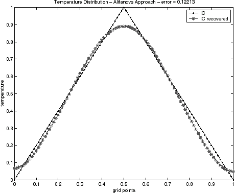
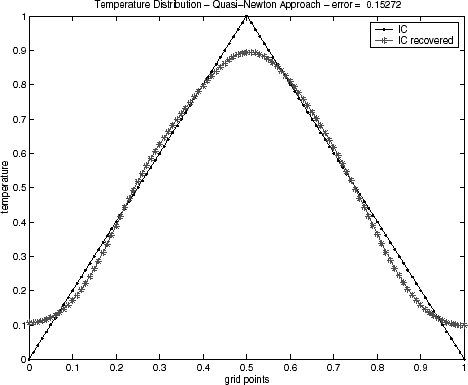
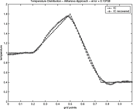
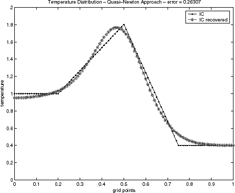
Initial condition reconstructions for the triangular test function – Eq. (37) – and for semitriangular test function – Eq. (38) – using noiseless data are shown in Figs. 1–4 and Figs. 5–8, respectively. The Alifanov's approach as well as the quasi-Newton's method provide good recoveries of the initial condition, while the GA method has been showing inadequate when the regularization operator is not applied. This behavior has been observed for both test functions. Similar results for GA algorithm have also been noticed in a recent lecture [29].

FIGURE 1 Alifanov's approach solution for the triangular function without regularization.

FIGURE 2 Quasi-Newton method solution for the triangular function without regularization.

FIGURE 3 Genetic algorithm solution for the triangular function without regularization: epidemical operator nonactivated.

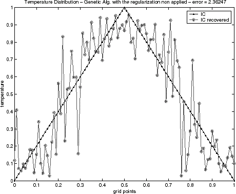
FIGURE 4 Genetic algorithm solution for the triangular function without regularization: epidemical operator activated.

FIGURE 5 Alifanov's approach solution for the semitriangular function without regularization.

FIGURE 6 Quasi-Newton method solution for the semitriangular function without regularization.

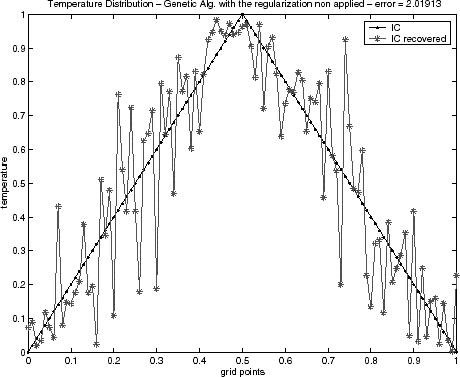
FIGURE 7 Genetic algorithm solution for the semitriangular function without regularization: epidemical operator nonactivated.

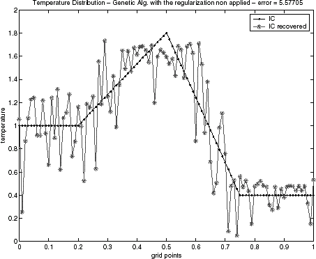
FIGURE 8 Genetic algorithm solution for the semitriangular function without regularization: epidemical operator activated.

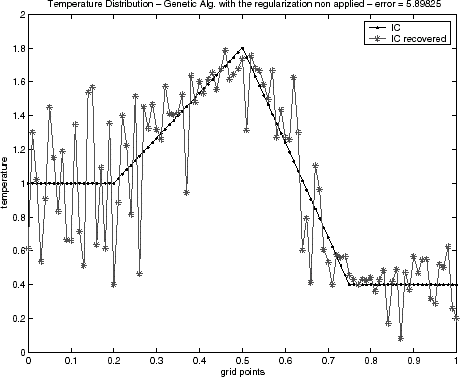
Table I presents a quantitative comparison of the techniques employed by the error value, defined by Eq. (40) with ξ = 0 (no regularization), when the noiseless data (σ = 0) is used. It can be noticed that the Alifanov's approach presents errors of an order of magnitude smaller when compared with the quasi-Newton method.

4.2 Noisy Data

Since the spatial resolution is M = 101, according to Morozov's discrepancy principle, the optimum regularization parameter ξ ^⋆ must be chosen in such a way that .

The optimization problem defined in Eq. (31) is iteratively solved by the quasi-Newton optimization algorithm presented in Section 3.2. The parameter vector has been always subjected to the following simple bound: 0 ≤ f_j ≤ 2.0, for triangular and semitriangular test functions. Regarding the GA method, the problem solved is defined in Eq. (34) and the parameters employed in this technique has been: tournament selection operator; geometrical crossover operator (μ = 1/2); nonuniform mutation operator (b = 5, l _inf = 0, l ^sup = 2.0), mutation probability of 5%; fixed population size of 400 individuals; and fixed maximal generation number of 50 000.

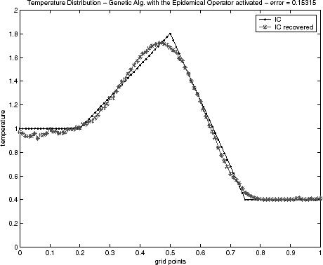
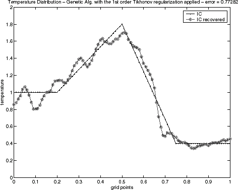
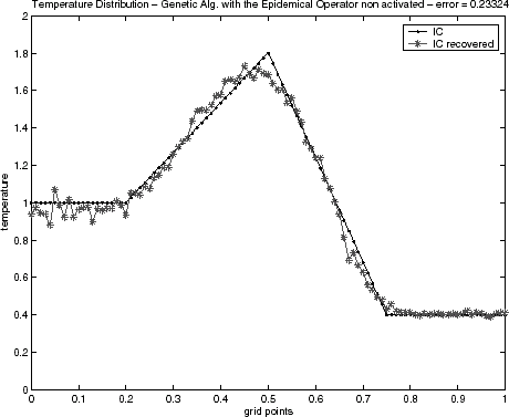
In relation to the estimations of the initial condition, Figs. 9–12 for the triangular test function and Figs. 14–17 for semitriangular test function present good results, even in the case when the GA technique without activating the epidemical operator is applied. The results for the triangular test function with the first order Tikhonov regularization, Fig. 13, were equivalent to the epidemic GA. However, results for the semitriangular test function, Fig. 18, were worse than epidemic GA, and even for the GA when the epidemical operator is not activated. The results have been obtained with the same maximal generation number used when the epidemical strategy of epidemic has been activated. Table II presents a quantitative comparison of the techniques employed by the error value defined by Eq. (40), when the noisy data is used.

FIGURE 9 Alifanov's approach solution for the triangular function.

FIGURE 10 Quasi-Newton method solution for the triangular function.

FIGURE 11 Genetic algorithm solution for the triangular function with the epidemical operator nonactivated.

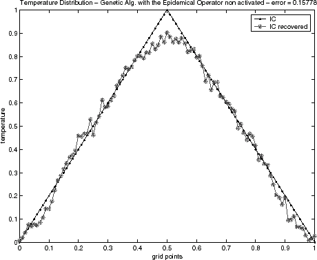
FIGURE 12 Genetic algorithm solution for the triangular function with the epidemical operator activated.

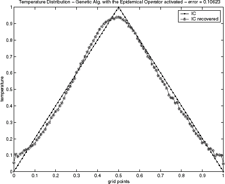
FIGURE 13 Genetic algorithm solution for the triangular function with the first order Tikhonov regularization: epidemical operator nonactivated.

FIGURE 14 Alifanov's approach solution for the semitriangular function.

FIGURE 15 Quasi-Newton method solution for the semitriangular function.

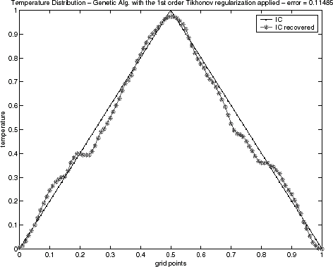
FIGURE 16 Genetic algorithm solution for the semitriangular function with the epidemical operator nonactivated.

FIGURE 17 Genetic algorithm solution for the semitriangular function with the epidemical operator activated.

FIGURE 18 Genetic algorithm solution for the semitriangular function with the first order Tikhonov regularization: epidemical operator nonactivated.

5 Final Comments

The inverse problem of estimating the unknown initial condition in a one-dimensional slab has been solved using three different techniques: the conjugate gradient method with the adjoint equation, regularized solution using a quasi-Newton method, and regularized solution by means of the GA method. All techniques employed here are based on the minimization of a functional form, and they were tested for two test functions: triangular and semitriangular, and for noiseless data and 5% noisy data. All techniques yielded good results for both test functions, except the GA, when the noiseless data is used and the regularization is not applied. However, the Alifanov's approach presented the best inverse solution. Considering the Alifanov's approach, the triangular test function presented the smoother estimate, whereas the semitriangular test function has more discontinuity in the derivative. The Morozov's discrepancy principle was useful to estimate the regularization parameter in the analyzed cases.

Contrasting with smoother solutions obtained with Alifanov's approach, regarding to the regularized solutions, it should be noted that the sensitivity and adjoint problems could become difficult to obtain in a general multidimensional and nonlinear inverse problem. In addition, better regularized solutions have been obtained with other regularization operators, such as higher order entropic regularization [6], as well the use of a nonextensive entropy [30].

The main purpose of using stochastic schemes for solving optimization problems is to reach the global minimum, avoiding a fall in local minima. In the case of the GA approach, the epidemical strategy was a more effective technique to find a more precise and smoother inverse solution.

Finally, a regularization operator has been necessary for the application of the GA approach, even working with noiseless data. This behaviour has also been noticed in a recent lecture [29]. However, dealing with noiseless data, the regularization operator has not been necessary to retrieve the initial condition when the quasi-Newtonian optimizer [27] has been employed.

Acknowledgments

The authors are gratefully indebted to FAPESP and CNPq, Brazilian agencies for research support. The authors would like to thank Profs. Keith A. Woodbury (The University of Alabama, USA) and Antonio J. Silva Neto (State University of the Rio de Janeiro, Brazil).

Additional information

Notes on contributors

Leonardo D. Chiwiacowsky*

*E-mail: [email protected]

Notes

*E-mail: [email protected]

OBS: *Refers to the case when the epidemical operator was not activated.

OBS: *Refers to the case when the epidemical operator was not activated.

^†Refers to the case when the first order Tikhonov regularization operator has been used.

References

- Hadamard J. 1923 Lectures on the Cauchy Problem in Linear Partial Differential Equations Yale Universtity Press New Haven
- Woodbury K.A. What are Inverse Problems? [http://www.me.ua.edu/whatis.html]
- Campos Velho H.F. 2001 Inverse problems: basic concepts and applications, short course Computational Modeling Meeting IV Polytechnic Institute, University of the State of the Rio de Janeiro 12–14 November Nova Friburgo (RJ) Brazil [http://www.lac.inpe.br/∼harddo/scip/html]
- Muniz W.B. 1998 Um problema inverso em conduçcão do calor utilizando métodos de regularização M.Sc. Thesis on Applied Mathematics UFRGS Porto Alegre Brazil
- Muniz , W.B. , Campos Velho , H.F. and Ramos , F.M. 1999 . A comparison of some inverse methods for estimating the inital condition of the heat equation . J. Comput. Appl. Math. , 103 : 145 – 163 .
- Muniz , W.B. , Ramos , F.M. and Campos Velho , H.F. 2000 . Entropy- and Tikhonov-based regularization techniques applied to the backwards heat equation . Comput. Math. Appl. , 40 : 1071 – 1084 .
- Silva Neto A.J. Özisik M.N. 1993 An inverse heat conduction problem of estimating initial condition Proceedings of the 12th Brazilian Congress of Mechanical Engineering (COBEM'93) pp. 613–616 Brasília Brazil
- Alifanov , O.M. 1974 . Solution of an inverse problem of heat conduction by iteration methods . J. Eng. Phys. , 26 : 471 – 476 .
- Alifanov , O.M. and Mikhailov , V.V. 1978 . Solution of the nonlinear inverse thermal conductivity problem by iteration method . J. Eng. Phys. , 35 : 1501 – 1506 .
- Jarny , Y. , Özisik , M.N. and Bardon , J.P. 1991 . A general optimization method using adjoint equation for solving multidimensional inverse heat conduction . Int. J. Heat Mass Tran. , 34 : 2911 – 2919 .
- Holland J.H. 1975 Adaptation in Natural and Artificial Systems University of Michigan Press Ann Arbor
- Goldberg D.E. 1989 Genetic Algorithms in Search, Optimization, and Machine Learning Addison-Wesley Publishing Company Inc. USA
- Michalewicz Z. 1996 Genetic Algorithms + Data Structures = Evolution Programs Springer-Verlag USA
- Mitchell M. 1996 An Introduction to Genetic Algorithms MIT Press USA
- Navarro P.L.G. Oliveira P.P.B. Ramos F.M. Campos Velho H.F. 1999 Magnetotelluric inversion using problem-specific genetic operators Proceedings of the Genetic and Evolutionary Computation Conference (GECCO-99) pp. 1580–1587 San Francisco USA
- Navarro P.L.G. Oliveira P.P.B. Ramos F.M. Campos Velho H.F. 2000 An evolutionary approach in magnetotelluric inversion 3rd International Conference on Inverse Problems in Engineering (3ICIPE) pp. 459–464 Port Ludlow Washington USA
- Barbosa H.J.C. Borges C.C.H. 2001 A genetic algorithm for damage identification in framed structures usign vibration data Proceedings of the IX International Symposium on Dynamic Problems of Mechanics – IX DINAME Florianópolis Brazil
- Campos Velho , H.F. and Ramos , F.M. 1997 . Numerical inversion of two-dimensional geoelectric conductivity distributions from eletromagnetic ground data . Braz. J. Geophys. , 15 : 133 – 143 .
- Ramos , F.M. , Campos Velho , H.F. , Carvalho , J.C. and Ferreira , N.J. 1999 . Novel approaches on entropic regularization . Inverse Probl. , 15 : 1139 – 1148 .
- Tikhonov A.N. Arsenin V.Y. 1977 Solutions of Ill-Posed Problems Winston & Sons Washington D.C
- Özisik M.N. 1980 Heat Conduction Wiley Interscience USA
- Carslaw H.S. Jaeger J.C. 1959 Conduction of Heat in Solids Oxford University Press London
- Silva Neto A.J. Moura Neto F.D. 2000 Choosing models: inverse problems in engineering, short course Brazilian Congress on Computational and Applied Mathematcis 11–15 September Santos (SP) Brazil (in portuguese)
- Alifanov , O.M. and Egorov , Y.V. 1985 . Algorithm and results of solving the inverse heat-conduction boundary problems in a two-dimensional formulation . J. Eng. Phys. , 48 : 489 – 496 .
- Morozov V.A. 1993 Regularization Methods for Ill-posed Problems Michael Stessin New York
- Morozov , V.A. 1966 . On the solution of functional equations by method of regularization . Soviet Math. Dokl. , 7 : 414 – 417 .
- E04UCF 1993 NAG Fortran Library Mark 13 Oxford UK
- Eshelman L. Schaffer J. 1993 Real-coded genetic algorithms and interval schemata Foundations of Genetic Algorithms 2 pp. 187–202 Morgan Kaufmann Publishes San Francisco
- Woodbury K.A. 2002 Application of genetic algorithms and neural networks to the solution of inverse heat conduction problems: a tutorial 4th International Conference on Inverse Problems in Engineering: Theory and Practice (ICIPE-2002) 26–31 May Angra dos Reis (RJ) Brazil [http://www.me.ua.edu/inverse]
- Shiguemori E.H. Campos Velho H.F. Silva J.D.S. Ramos F.M. 2002 A parametric study of a new regularization operator: non-extensive entropy 4th International Conference on Inverse Problems in Engineering: Theory and Practice (ICIPE-2002) 26–31 May Angra dos Reis (RJ) Brazil