Abstract
This article describes a methodology for using neural networks in an inverse heat conduction problem. Three neural network (NN) models are used to determine the initial temperature profile on a slab with adiabatic boundary condition, given a transient temperature distribution at a given time. This is an ill-posed one-dimensional parabolic inverse problem, where the initial condition has to be estimated. Three neural network models addressed the problem: a feedforward network with backpropagation, radial basis functions (RBF), and cascade correlation. The input for the NN is the temperature profile obtained from a set of probes equally spaced in the one-dimensional domain. The NNs were trained considering a 5% of noise in the experimental data. The training was performed considering 500 similar test-functions and 500 different test-functions. Good reconstructions have been obtained with the proposed methodology.
1. Introduction
Neural networks have emerged as a new technique in solving inverse problems. This approach was used to identify initial conditions in an inverse heat conduction problem on a slab with adiabatic boundary conditions, from transient temperature distribution, obtained at a given time. Three neural networks (NNs) architectures have been proposed to address the problem: the multilayer perceptron with backpropagation, radial basis functions (RBF), both trained with the whole temperature history mapping, and cascade correlation.
The results are compared with those obtained with nonlinear least square approach and standard regularization schemes [Citation1, Citation2].
Preliminary results using backpropagation and radial basis function neural networks were obtained using whole time history, but with only three different test-functions for the learning process [Citation3, Citation4]. The reconstructions obtained were worse than those identified with regularization techniques. In that strategy two NNs were coupled: the first NN was used for determining the time-period to get the observational data, and another one to find the initial condition itself. That strategy constituted in a novelty in the field, but in all probability the poor set of test-functions for learning step did not permit a good reconstruction. In order to overcome this constraint, 500 functions were used for the learning process in this work. In addition, two groups of test-functions were used. In the first group 500 completely different test-functions were used, while for the second group 500 similar test-functions were used.
Numerical experiments were carried out with synthetic data with 5% of noise which was used to simulate experimental data.
2. Direct Heat Transfer Problem
The direct problem under consideration consists of a transient heat conduction problem in a slab with adiabatic boundary condition, with an initial temperature profile denoted by f (x). Mathematically, the problem can be modeled by the following heat equation
The direct problem solution, for a given initial condition f (x) is explicitly obtained using separation of variables, for (x,t) ∈ Ω × R+:
The inverse problem consists of estimating the initial temperature profile f (x) for a given transient temperature distribution T (x, t) at a time t [Citation1].
3. Neural Network Architectures
Artificial neural networks (ANNs) are made of arrangements of processing elements (neurons). The artificial neuron model basically consists of a linear combiner followed by an activation function. Arrangements of such units form the ANNs that are characterized by:
| 1. | Very simple neuron-like processing elements; | ||||
| 2. | Weighted connections between the processing elements (where knowledge is stored); | ||||
| 3. | Highly parallel processing and distributed control; | ||||
| 4. | Automatic learning of internal representations. | ||||
Artifical neural networks aim to explore the massively parallel network of simple elements in order to yield a result in a very short time slice and, at the same time, with insensitivity to loss and failure of some of the elements of the network. These properties make artificial neural networks appropriate for application in pattern recognition, signal processing, image processing, financing, computer vision, engineering, etc. [Citation6–Citation9].
The simplest ANN model is the single-layer Perceptron with a hard limiter activation function, which is appropriate for solving linear problems. This fact prevented neural networks of being massively used in the 1970s [Citation6]. In the 1980s they reemerged due to Hopfield's paper on recurrent networks and the publication of the two volumes on parallel distributed processing (PDP) by Rumelhart and McClelland [Citation6].
There exist ANNs with different architectures that are dependent upon the learning strategy adopted. This article briefly describes the three ANNs used in our simulations: the multilayer Perceptron with backpropagation learning, radial basis functions (RBF), and cascade correlation. A detailed introduction on ANNs can be found in [Citation6,Citation9].
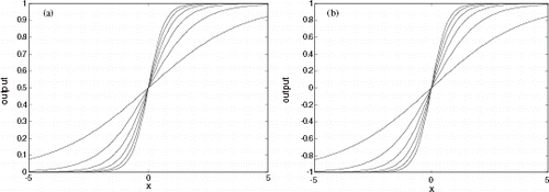
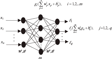
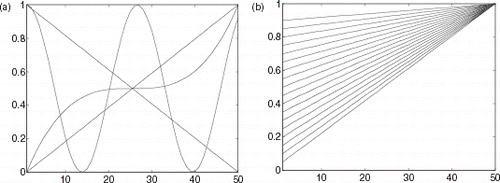
Multilayer perceptrons with a backpropagation learning algorithm, commonly referred to as backpropagation neural networks, are feedforward networks composed of an input layer, an output layer, and a number of hidden layers, whose aim is to extract high order statistics from the input data [Citation4]. Figure 2 depicts a backpropagation neural network with a hidden layer. Functions g and f provide the activation for the hidden layer and the output layer neurons, respectively. Neural networks will solve nonlinear problems, if nonlinear activation functions are used for the hidden and/or the output layers. Figure 1 shows examples of such functions.
A feedforward network can input vectors of real values onto output vectors of real values. The connections among the several neurons (Fig. 2) have associated weights that are adjusted during the learning process, thus changing the performance of the network. Two distinct phases can be devised while using an ANN: the training phase (learning process) and the run phase (activation of the network). The training phase consists of adjusting the weights for the best performance of the network in establishing the mapping of many input–output vector pairs. Once trained, the weights are fixed and the network can be presented to new inputs for which it calculates the corresponding outputs, based on what it has learned.
The backpropagation training is a supervised learning algorithm that requires both input and output (desired) data. Such pairs permit the calculation of the error of the network as the difference between the calculated output and the desired vector. The weight adjustments are conducted by backpropagating such error to the network, governed by a change rule. The weights are changed by an amount proportional to the error at that unit, times the output of the unit feeding into the weight. Equation (3) shows the general weight correction according to the so-called Delta rule
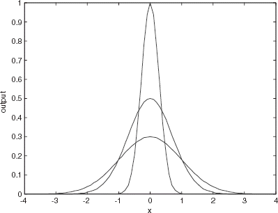
Radial basis function networks are feedforward networks with only one hidden layer. They have been developed for data interpolation in multidimensional space. RBF nets can also learn arbitrary mappings. The primary difference between a backpropagation with one hidden layer and an RBF network is in the hidden layer units. RBF hidden layer units have a receptive field, which has a center, that is, a particular input value at which they have a maximal output. Their output tails off as the input moves away from this point. The most used function in an RBF network is a Gaussian (Fig. 3).
Radial basis function networks require the determination of the number of hidden units, the centers, and the sharpness (standard deviation) of their Gaussians. Generally, the centers and standard deviations are decided on first by examining the vectors in the training data. The output layer weights are then trained using the Delta rule.
The training of RBF networks can be conducted: (1) on classification data (each output representing one class), and then used directly as classifiers of new data; and (2) on a pair of points (x, f (x)) of an unknown function f, and then used to interpolate. The main advantage of RBF networks relies on the fact that one can add extra units with center near elements of the set of input data, which are difficult to classify.
Like backpropagation networks, RBF networks can be used for processing time-varying data and many other applications.
The third ANN used in this article is the cascade correlation. This NN permits dynamically to find out the appropriated number of neurons, begining with just the input and output layers, with all the neurons fully interconnected (there is no hidden layer). The weights on these connections are determined using a conventional learning. Next, new neurons are considered sequentially, and weights between the candidate units and the inputs are selected to maximize the correlation between the activation of the neuron(s) and the residual error of the net. Once a neuron is selected, its weights on the inputs are frozen, and are not subsequently changed when considering new neurons. Additional neurons are applied until a specified small error is reached.
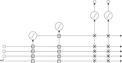
Figure 4 shows a cascade correlation (CasCor) network into which two candidate neurons have been implemented. These neurons use a conventional activation function, as shown in Fig. 2. Each open box in the figure represents a weight that is trained only once (when the neuron is a candidate) and then is frozen. But the cross marks represent weights that are repeatedly changed as the network evolves. Note that the structure of the network is such that the inputs remain directly connected to the outputs, but also some information is filtered through the neurons. The direct input to output connection can handle the linear portion of the mapping, while the nonlinearities are addressed by the neurons.
4. Neural Network for Determining the Initial Condition
Artificial neural networks have two stages in their application, firstly the learning and then activation steps. During the learning step, the weights and bias corresponding at each connection are adjusted to some reference examples. For activation, the output is obtained based on the weights and bias computed in the learning phase. A supervised learning was used for all NN architectures.
The numerical experiment for inverse problem is based on two test-functions, the triangular function
The experimental data (measured temperatures at a time τ > 0), which intrinsically contains errors in the real world, is obtained by adding a random perturbation to the exact solution of the direct problem, such that
Twin numerical experiments were performed. In the first one, a noiseless observational data were employed (σ = 0). For the second numerical experiment was carried out using 5% of noise (σ = 0.05).
For the NNs, the training sets are constituted by synthetic data obtained from the forward model, i.e., profile of a measure points from probes spread in the space domain. Two different data sets were used. The first data set is the profiles obtained from 500 similar functions (see examples in Fig. 5b). The second one is that obtained with 500 non-similar functions Fig. 5a). Similar functions are those belonging to the same class (linear function class, trigonometric function class, such as sine functions with different amplitude and/or phase, and so on). Non-similar functions are those completely different, in which each one belonging to a distinct class.
Figure 5 shows a set of functions used in the learning stage, applying non-similar (Fig. 5a) and similar functions (Fig. 5b).
The activation is a regular test used for checking out the NN performance, where a function belonging to the test-function set is applied to activate (to run) the NN. Good activations were obtained for all three NNs for observational data with noise and noiseless data, for similar and non-similar test-function sets (not shown). In the activation test the NN trained with similar data were systematically better than the training with non-similar functions (not shown too), with and without noise in the data. A summary of the training results for three NNs is presented in .
TABLE I Training results for the neural networks used for initial condition reconstruction
Nevertheless, the activation test is an important procedure, indicating the performance of an NN, the effective test is defined using a function (initial condition) that did not belong to the training function set. This action is called the generalization of the NN. Functions as expressed by Eqs. (4) and (5) did not belong to the function set in the training step.
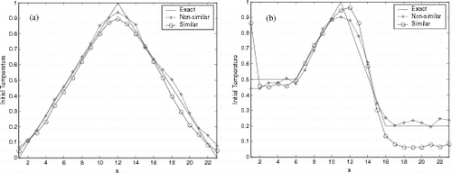
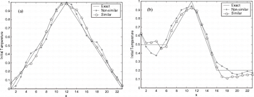
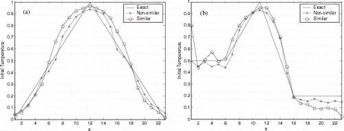
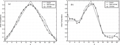
Figures 6–8 show the initial condition reconstruction for noiseless experimental data, and presents the Average Square Error (ASE) for three NNs used in this article. Differently from the results for the activation test, reconstruction using non-similar functions were better than estimation with similar functions.
TABLE II Activation results for the noiseless experimental data
The poorer reconstructions for noiseless data were obtained using CasCor NN (see and Figures 6–8), and the best identifications were obtained using RBF NN. However, good initial condition identifications were obtained with three NN architectures.
Real tests for inverse problems must be performed using some level of noise in the synthetic experimental data. As was mentioned, the real experimental data were simulated corrupting the output data from direct problem with Gaussian white noise, see Eq. (6).
As with our numerical experiment with noiseless data, the identification of the initial condition was effective for all NNs used here.
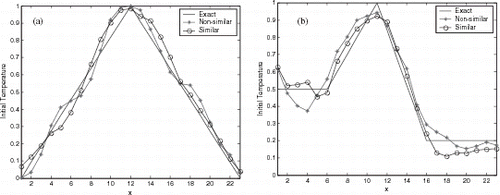
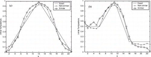
Figures 9– show the reconstructions for multilayer perceptron, RBF and CasCor NNs. presents the ASE for two test-function in the generalization. As expected the reconstruction with data contaminated with noise was worse than noiseless data. But the NNs were robust in the identification with noise in the experimental data.
TABLE III Activation results for the experimental data with 5% of noise
5. Final Remarks
Three architectures of neural networks were studied in the reconstruction of the initial condition of a heat conduction problem. All of the NNs were effective for solving this inverse problem. Different from previous results [Citation3, Citation10], reconstructions are comparable with those obtained with regularization methods [Citation2], even for data containing noise. However, the NNs do not remove the inherent ill-posedness of the inverse problem.
The initial condition estimation problem is a harder inverse problem than the identification of a boundary condition in heat transfer [Citation11–Citation13].
An interesting remark is the result for the activation test, where the training with similar functions produced better identification than non-similar function. However, reconstructions using non-similar functions were systematically better for the generalization, except in only one case: the estimation of semi-triangular function by RBF NN with 5% of noise ().
The worse estimation was obtained with CasCor NN. A future work could be done using the strategy adopted by Hidalgo and Gómez-Treviño [Citation14]. To accommodate large amounts of noise, they added a regularization term to the least squares objective function of the neural network.
Processing with NNs is a two step process: training and activation. After the training phase, the inversion with NNs is much faster than the regularization methods, and the NNs do not need a mathematical model to simulate the forward model. In addition, NNs is an intrinsically parallel algorithm. Finally, NNs can be implemented in hardware devices, the neurocomputers, becoming the inversion processing faster than NNs emulated by software.
Nomenclature
Table
References
References
- Muniz , WB , de Campos Velho , HF and Ramos , FM . 1999 . A comparison of some inverse methods for estimating the initial condition of the heat equation . J. Comp. Appl. Math , 103 : 145
- Muniz , WB , Ramos , FM and de Campos Velho , HF . 2000 . Entropy- and Tikhonov-based regularization techniques applied to the backwards heat equation . Comp. Math. Appl , 40 : 1071
- Issamoto E Miki FT da Luz JI da Silva JD de Oliveira PB de Campos Velho HF 1999 An inverse initial condition problem in heat conductions: a neural network approach Braz. Cong. Mech. Eng. (COBEM), Proc. in CD-ROM – paper code AAAGHA 238 Unicamp, Campinas (SP) Brasil
- Miki FT Issamoto E da Luz JI de Oliveira PB de Campos Velho HF da Silva JD 1999 A Neural network approach in a backward heat conduction problem Braz. Conf. Neural Networks. Proc. in CD-ROM – paper code 0008 019 São José dos Campos (SP) Brasil
- Özisik MN 1980 Heat Conduction, Wiley Interscience
- Haykin S 1994 Neural Networks: A Comprehensive Foundation., Macmillan New York
- Lin C-T Lee G 1996 Neural Fuzzy Systems: A Neuro-Fuzzy Synergism to Intelligent Systems, Prentice Hall New Jersey
- Nadler M Smith EP 1993 Pattern Recognition Engineering, John Wiley and Sons New York
- Tsoukalas LH Uhrig RE 1997 Fuzzy and Neural Approaches in Engineering, John Wiley and Sons New York
- Miki FT Issamoto E da Luz JI de Oliveira PB de Campos Velho HF da Silva JD 2000 An inverse heat conduction problem solution with a neural network approach Bulletin of the Braz. Soc. for Comp. Appl. Math (SBMAC). Available in the internet: www.sbmac.org.br/publicacoes
- Krejsa , J , Woodbury , KA , Ratliff , JD and Raudensky , M . 1999 . Assessment of strategies and potential for neural networks in the IHCP . Inverse Probl. Eng , 7 : 197
- Woodbury KA 2000 Neural networks and genetic algorithms in the solution of inverse problems Bulletin of the Braz. Soc. for Comp. Appl. Math (SBMAC). Available in the internet: www.sbmac.org.br/publicacoes
- Shiguemori EH Harter FP de Campos Velho HF da Silva JDS 2001 Estimation of boundary conditions in heat transfer by neural networks Braz. Cong. on Comp. and Appl. Math 559 Belo Horizonte (MG) Brazil
- Hidalgo , H and Gómez-Trevińo , E . 1996 . Application of constructive learning algorithms to the inverse problem . IEEE T. Geosci. Remote , 34 : 874
