On stable iterative methods of gradient type for the inverse medium scattering problem

Abstract

In this article we present a class of iterative methods for the inverse problem of 3D acoustic scattering on a penetrable inhomogeneity. We formulate the problem as an ill-posed nonlinear operator equation in a Hilbert space. The proposed methods are based on an approximation of this equation by a strongly convex finite-dimensional variational problem. The strong convexity of the approximating problem plays the key role in a theoretical justification of our approach to numerical approximation of solutions to ill-posed problems. Specifically, this property ensures the stability of the proposed iterative methods with respect to the errors in input data as an iteration number increases. We also present results of computational experiments.

Keywords:

• Inverse scattering problem
• Ill-posed problem
• Operator equation
• Stable iterative methods

1. Problem formulation

This article is concerned with a numerical analysis of the inverse medium scattering problem for acoustic waves. The problem is to determine a refractive index of an inhomogeneous medium from the measurements of far-field patterns of scattered time-harmonic acoustic waves.

We work with the classical model of time-harmonic acoustic scattering on an inhomogeneity [1, Ch. 8]. Assume that a 3D homogeneous acoustic medium consists of a penetrable inhomogeneous inclusion localized within a bounded open subset B ⊂R³. Acoustical properties of the medium are characterized by the sound speed c(x) > 0, x∈ R³. Assume that the sound speed outside B is a given constant c₀ : c(x)  = c₀ , x ∈ R³\B. Therefore the medium can be described by the refractive index (---203---1) Suppose n belongs to the Sobolev space H^s (B) with s > 3 / 2. For an introduction to Sobolev spaces, we refer to [2]. By the embedding theorem, n(x) satisfies the Hölder condition: (---203----1) for all x, y ∈ B with L₀ > 0 and an appropriate α  independent of x, y. The scattering of an incident time-harmonic plane wave with the complex amplitude (---203----2) is described by the equations (---203--1) (---203---2) and the Sommerfeld radiation condition (---203--2) where x · y stands for the scalar product of vectors x, y ∈ R³, k > 0 is the wavenumber fixed throughout the article, (---203----3) R³: (---203----4) is the direction of motion of the incident wave, and u(x, d) and u_s (x, d) are complex amplitudes of the full and scattered wave field, respectively. The Sommerfeld condition guarantees that the scattered wave is outgoing. In the direct scattering problem, the refractive index n = n(x), x ∈ B is given and the full wave field u(x, d) or the scattered field u_s (x, d), x ∈  R³ is to be evaluated. It is well known (see [1, Ch. 8]) that this problem has a unique solution. Moreover, for the scattered field the following asymptotic representation is valid [1, p. 222] (---203--3) The factor (---203----5) in (3)(---203--3) is called the far-field pattern or the scattering amplitude of u_s (x, d) and the unit vector (---203----6) is the direction of observation of u_s (x, d). Denote a(x) = 1 − n(x), then we obviously have a(x)  = 0 for x ∈  R³\B and (---203----7) .

The inverse medium acoustic scattering problem is to determine the refractive index (---203----8) or, equivalently, the function (---203----9) given the scattering amplitudes (---203----10) for all directions d ∈S² of incoming plane waves. Hence the input data of the problem under consideration are the values (---203----11) for all (---203----12) . It can be shown [1, p. 278] that the inverse acoustic problem in this setting has a unique solution, i.e., the refractive index n(x) is uniquely determined by the knowledge of the far-field patterns (---203----13) .

Recall that the direct scattering problems (1)(---203--1) and (2)(---203--2) is equivalent to the Lippmann–Schwinger equation [1, p. 216] (---203--4) where (---203---3) is the fundamental solution of the Helmholtz equation in a homogeneous space (n(x) ≡ 1, x∈R³) subject to the Sommerfeld condition (2)(---203--2) . Multiplying both the parts of (4)(---203--4) by a(x), as in [3] we come to the equality (---203--5) where (---203----14) . With the use of notation (---203---4) we can rewrite (5)(---203--5) as (---203---5) where I stands for the identity operator and a denotes the operator of multiplication by a(x). It is easily seen that if v(x, d) solves equation (5)(---203--5) then the function (---203----15) satisfies (1)(---203--1) and (2)(---203--2) . Since by (4)(---203--4) , (---203---6) for the scattering amplitude (---203----16) we then have the representation [1, p. 223] (---203--6) where the operator E is defined by the equality (---203---7) Combining (5)(---203--5) and (6)(---203--6) , we come to the following nonlinear equation for the unknown function a(x), x ∈B (---203--7)

It is well known [1, Ch. 10] that equation (7)(---203--7) is an ill-posed problem for each reasonable choice of the solution space and the space of right-hand side in (7)(---203--7) . This problem is usually studied in the Lebesgue space L₂ , Sobolev spaces (---203----17) , or the spaces of smooth functions (---203----18) . The ill-posedness of (7)(---203--7) means that arbitrarily small variations of the scattering amplitudes (---203----19) can lead to significant changes in solution a(x) or can even transform (7)(---203--7) into an equation that has no solutions at all. Hence for stable numerical approximation of a solution to (7)(---203--7) one should use regularization methods (see, e.g., [4–6]). A widely accepted class of such methods make up iterative regularization algorithms. Algorithms of this type are very attractive in practice because of the ease of their numerical implementation especially when a solution space of the problem is Hilbert space L₂ . The monograph [6] presents a number of iterative procedures for nonlinear ill-posed equations with smooth operators given with errors. However, the convergence of the methods of [6] is established under rather severe conditions on the operators of equations. These conditions involve the first derivative of the operators and generalize the classical regularity condition, which says that the derivative must be continuously invertible. When applied to the inverse problems of potential theory and inverse acoustical problems including (7)(---203--7) , none of such conditions has been verified so far (see [7–9]). Moreover, on a solution space L₂ , which is formally most convenient for numerical treatment, operators of applied inverse problems often possess fewer smoothness properties than are required by existing convergence theorems. In particular, these operators usually appear to be well defined not on the whole of the space of L₂ -functions but on its subsets of continuous or smooth functions [1, Chs. 5, 8]. This fact raises additional difficulties for rigorous theoretical justification of iterative solution methods for such inverse problems.

In the present article we propose a general scheme of constructing iterative methods for solving nonlinear ill-posed equations without any assumptions concerning the differentiability of their operators on open subsets of the solution space. The iterative points generated by the proposed methods are attracted to a small neighborhood of the solution. In other words, these methods appear to be stable with respect to the errors of input data. The stabilization of iterations is ensured by an appropriate finite-dimensional approximation of the original equation. We also give results of computational experiments with some of the proposed methods in application to the inverse acoustical problem described above. The article is organized as follows: in Section 2 we present a sketch of the abstract scheme and describe the proposed methods for solving (7)(---203--7) ; Section 3 contains the results of our computational tests.

2. A class of iterative methods

In this section we consider the operator equation (---203--8) where (---203----20) is a nonlinear operator and H₁ , H₂ are the Hilbert spaces. Fix arbitrarily an element ξ ∈H₁ and choose a finite-dimensional subspace M ⊂ H₁. The pair (---203----21) will be used below for constructing a regular finite-dimensional approximation of the original problem (8)(---203--8) . We shall consider M as a Euclidean space endowed with the norm of H₁. Let u* be a solution of (8)(---203--8) and P_M be the orthoprojector from H₁ onto M. Assume that (---203--9) The value Δ estimates an error of approximation of u* by the affine subspace M_ξ , where (---203---8) Throughout the article, ‖·‖ _H stands for the norm of a Hilbert space H; L(H₁ , H₂ ) is the Banach space of all linear bounded mappings from H₁ into H₂. We endow L(H₁ , H₂ ) with the standard norm (---203---9) No assumptions are made both on a differentiability of the operator F(u) in an open neighborhood of u* and on a continuous invertibility of the derivative F′(u) if F(u) is differentiable. Therefore, equation (8)(---203--8) represents a very general abstract model of applied ill-posed problems. Instead of the classical smoothness assumptions we impose on F(u) the weaker condition that (---203---10) and the operator (---203---11) is Fréchet differentiable with a Lipschitz continuous derivative, at least for points u ∈M from a neighborhood of (---203----22) . More comprehensively, suppose that for some positive constants L = L(M) and R we have (---203--10) where by definition (---203----23) . Also, suppose the operator (---203---12) is Fréchet differentiable at the point (---203----24) and the derivative (---203----25) satisfies the condition (---203--11) then the operators Φ ′(u) and Ψ′(u) are understood as linear continuous mappings from M into H₂. Note that if F(u) appears to be differentiable on H₁ then we have (---203----26) and (---203----27) . Let us impose on M the following additional restriction:

Assumption A The subspace M is chosen such that the linear operator (---203----28) is injective, i.e., one-to-one.

Assumption A implies that the operator F(u) must be regular as a mapping from (---203----29) into H₂ but not necessarily from the whole of H₁ into H₂ as classical regularity assumptions require. In the case that F(u) is differentiable on an open neighborhood of u*, Assumption A simply means that F(u) is regular as a mapping from M_η into H₂ for all points η ∈H₁ sufficiently close to u*. In this situation it is obvious that Assumption A is valid for each subspace M ⊂ H₁ if the operator (---203----30) is injective. The last remark allows for the following generalization. Suppose (---203----31) is a Hilbert or Banach space embedded into H₁, the solution (---203----32) , the operator (---203----33) is differentiable on a neighborhood of u*, and the derivative (---203----34) is injective. Then Assumption A is valid for each finite-dimensional subspace (---203----35) . Let us remark that the operator F of the inverse medium scattering problem (7)(---203--7) satisfies the above listed conditions with the spaces (---203----36) (s > 3 / 2), H₁ = L₂ (B), and (---203----37) [3]. This fact partially motivates the choice of (7)(---203--7) as an object of our computational experiments.

Also, Assumption A is valid if F(u) is continuously differentiable and there exists a point (---203----38) in a small neighborhood of u* such that Ker (---203----39) , where Ker (---203----40) .

The lack of standard differentiability and regularity properties of the operator F(u) rises the question of stable evaluation of u* especially when F(u) is given approximately. Let (---203----41) be an available approximation of F(u). Assume that (---203----42) . Then instead of the true operator Φ (u) we have only its perturbation (---203----43) . Suppose the operator (---203----44) is Fréchet differentiable and the derivative (---203----45) satisfies (10)(---203--10) and the following conditions: (---203--12) where δ has the meaning of an error level in (---203----46) . Stable iterative methods that we intend to propose for solving (8)(---203--8) are based on approximation of the original equation (8)(---203--8) by the finite-dimensional variational problem (---203--13)

Denote by ρ = ρ (M) > 0 the least eigenvalue of the operator (---203---13) and set (---203---14) where N = N(M), r = r(M). The following theorem establishes the main qualitative property of the functional (---203----47) defined by (13)(---203--13) .

THEOREM 1 Let Assumption A and conditions (9)(---203--9) –(12)(---203--12) be satisfied. Suppose (---203--14) Then the functional (---203----48) is strongly convex on the finite-dimensional ball (---203----49) . Moreover, (---203----50) has a unique local minimum (---203----51) with (---203----52) , and the estimate is valid: (---203--15)

This assertion is an immediate consequence of Theorem 3 from [10]. Thus we see that if the conditions of Theorem 1 are satisfied then for practical minimization of (---203----53) over the finite-dimensional subspace M we can effectively use various iterative procedures, e.g., gradient processes, conjugate gradient methods, etc. (see, e.g. [11,12]). Since the functional (---203----54) is locally strongly convex, most of these methods starting at a point u₀ ∈M from a neighborhood of (---203----55) generate sequences (---203----56) such that (---203----57) and (---203----58) . Due to the strong convexity of (---203----59) , rate of convergence estimates for these methods are also available [11,12]. We can now characterize asymptotic properties of the sequences {u_n} with respect to the solution u* of (8)(---203--8) .

THEOREM 2 Let assumptions of Theorem 1 be satisfied. Suppose (---203--16) and the initial point u₀ ∈M satisfies (---203--17) Then the functional (---203----60) is strongly convex on the level set (---203---15)

Let {u_n} be a minimizing sequence for the functional (---203----61) such that (---203---16) with (---203----62) specified in Theorem 1. Then for the elements (---203----63) we have (---203--18)

The proof of Theorem 2 follows directly from the proof of Theorem 4 [10].

In order to clarify the statements of Theorems 1 and 2, let us assume as a preliminary that we have chosen and fixed the subspace M so that the value ρ = ρ (M) is a given constant. From (14)(---203--14) and (16)(---203--16) it follows that the conditions of the theorems can be fulfilled only if the values Δ, Δ₁, and (---203----64) are sufficiently small. On the other hand, estimates (15)(---203--15) and (18)(---203--18) become more informative when Δ and (---203----65) tend to zero. Since all these values depend on the choice of ξ, it is natural to consider (9)(---203--9) , (11)(---203--11) , and the inequality (---203----66) with small Δ, Δ₁, and Δ₂ as restrictions imposed on the element ξ. The theorems then imply that if an initial approximation (---203----67) is taken from a fixed neighborhood of (---203----68) (see (17)(---203--17) ), then the sequence {v_n} is attracted to a neighborhood of u* with diameter proportional to δ, Δ, and Δ₂ . Specifically, if ξ is chosen such that Δ and Δ₂ are of orderδ then Theorem 2 implies the stabilization of v_n in a neighborhood of diameter O(δ) while the starting point is taken arbitrarily from a ball of diameter O(1). For example, if ξ = ξ* satisfies (---203----69) then we get (---203----70) , and conditions (14)(---203--14) are equivalent to the upper bound of the error level: (---203----71) . In this case, (18)(---203--18) takes the form (---203---17) and hence the iterations v_n , n →∞ are attracted to a neighborhood of the solution u* with a diameter of orderδ. Although we have no rigorous algorithm for finding ξ*, inequality (18)(---203--18) shows that in a general situation when (---203----72) but Δ and Δ₂ are small, the sequence {v_n} (n →∞) behaves similarly provided that conditions (14)(---203--14) , (16)(---203--16) , and (17)(---203--17) are satisfied. To ensure these conditions, all available a priori information concerning the solution u* should be used. An algorithmic implementation of possible approaches to construction of (ξ , M) following by one or another volume of a priori information remains an open problem. Also, note that each algorithm that generates parametric families (---203----73) with the properties (---203---18) defines a regularization algorithm for the original equation [4–6]. Given the error levelδ this algorithm takes each approximate operator (---203----74) to the element (---203----75) specified in Theorem 1. Then by (15)(---203--15) we have (---203---19)

In view of the first condition from the listed above, it is likely that the family {M(δ)} must be chosen such that (---203----76) although formally speaking the increase of dim M(δ) is not necessary, since all the conditions can be in principle satisfied by a suitable choice of a position of a low-dimensional subspace M(δ) in H₁. Observe that variations of the parameter ξ (δ) provide additional means for minimization of (---203----77) .

Let us describe an abstract scheme of constructing stable iterative methods for equation (8)(---203--8) . First, pick a subspace M ⊂ H₁ satisfying Assumption A. Then using an available a priori information concerning u*, choose an element ξ ∈H₁ such that (---203----78) and inequalities (9)(---203--9) , (11)(---203--11) , and (---203----79) are valid with small Δ, Δ₁, and Δ₂ . Next, an iterative method for minimization of the locally strongly convex functional (---203----80) should be fixed. According to (18)(---203--18) , the iterations (---203----81) , where u_n are generated by the method, will be attracted to a neighborhood of u* with diameter of order O(δ+ Δ+ Δ₂ ).

For solving (13)(---203--13) various gradient-type procedures and other classes of iterative methods are applicable. As examples we only point at the well-known gradient iterations (---203--19) with a constant stepsize γ > 0 and Fletcher and Reeves' conjugate gradient method [11, Ch. 8] (---203--20) where γ_n > 0 is defined by the equality (---203---20) and the direction p_n is constructed in the form (---203---21)

Remark 1 In the case that D(F)  = H₁and the operator F(u) is differentiable on the whole of H₁, asymptotic properties of the process (19)(---203--19) and its variants were studied in [13, Ch. 5].

Remark 2 Theorems 1 and 2 remain valid if the condition (---203----82) is relaxed as follows: (---203---22) Concluding this section, we point out that for solving (13)(---203--13) some continuous analogs of classical iterative methods are also applicable. Among others we can use the gradient process (---203--21) which is the limit form of the iterations (19)(---203--19) as γ→0. From Theorem 1 it follows that if the initial point u₀ is sufficiently close to (---203----83) then the stationary point (---203----84) of the finite-dimensional dynamical system (21)(---203--21) is asymptotically stable and there exist constants C, ω > 0 such that (---203---23) Due to (15)(---203--15) , for elements (---203----85) we have the estimate (---203---24) If the operator (---203----86) is differentiable on an open neighborhood of u* then (21)(---203--21) takes the form (---203--22)

The process (22)(---203--22) can be considered as a continuous analog of the iterative methods recently studied in [13, Ch. 5].

In the next section we apply iterations (19)(---203--19) and (20)(---203--20) to the inverse medium scattering problem presented in Section 1.

3. Application to the inverse scattering problem

We are now ready to present several stable iterative methods for the equation (7)(---203--7) . In order to write (7)(---203--7) in the form of (8)(---203--8) , define the operator (---203---25) where (---203--23)

Suppose (---203----87) is a parallelepiped containing the inhomogeneity of the medium. For solving (8)(---203--8) with the operator (23)(---203--23) the processes (19)(---203--19) and (20)(---203--20) are applicable. We take (---203----88) ; as we choose M as the subspace of trigonometrical polynomials (---203--24) Denote by a* (x) the solution of (7)(---203--7) so that n* (x)  = 1 − a* (x) is the unknown refractive index of the inhomogeneity. Assume that instead of the true scattering amplitudes (---203----89) , some of their approximations (---203----90) are available. Thus the approximate operator (---203----91) has the form (---203---26)

As in [3], it can be easily shown that if the value (---203----92) is sufficiently small then with some ϵ > 0 we have (---203---27) and the Fréchet derivative Φ′(a) is Lipschitz continuous for all a from the neighborhood (---203----93) . Assumption A in this context is also satisfied since (---203----94) (s > 3 / 2) is an injective operator (see Proposition 2.2 in [3]), and (---203----95) . Using the representation (---203---28) we can rewrite (13)(---203--13) as the finite-dimensional optimization problem (---203---29) where (---203--25)

Here |z| stands for the modulus of z ∈ C. For evaluating the partial derivatives (---203----96) in (19)(---203--19) and (20)(---203--20) we used the standard finite-difference scheme (---203---30) with h = 10^− 3. When implementing the iterations (19)(---203--19) and (20)(---203--20) , we need to solve the direct scattering problem (5)(---203--5) several times per iteration. In our tests the equation (5)(---203--5) was solved by the simple iteration process (---203--26)

In all experiments the function (---203----97) was approximated by 8 iterations (26)(---203--26) with the stepsize λ = 0.5.

In order to define the functional (25)(---203--25) completely it suffices to specify the parameter (---203----98) . The best possible choice is evidently (---203---31) with an arbitrary ς ∈M^(N), but it is unlikely that any algorithmic ways to determine such ξ exist. Nevertheless, if the unknown solution a* (x)allows for a satisfactory approximation by the trigonometrical polynomials (24)(---203--24) then we can simply put ξ = 0. This is precisely the choice that we followed in our computational experiments.

We studied the model inverse scattering problem with the known exact solution n* (x)  = 1 − a* (x), where (---203---32) B₀ = (0, 4) × (0, 4) × (0, 4) is a domain actually containing the inhomogeneity and B  = (0, 6) × (0, 6) × (0, 6) is a given domain of R³ where the inhomogeneity a priori lies. The directions of observation (---203----99) and directions of incident waves d = d^(j) ranged over the set of 14 directions (---203---33) “uniformly” distributed over the sphere S² . The numerical integration over S² × S² in (25)(---203--25) was performed by the scheme (---203---34) with m = 14 and (---203----100) . To integrate over the parallelepiped B we chose the 3D Gauss scheme with 8 knots by each coordinate. In all the tests we put k  = 1 and (---203----101) so that the unknown function (---203----102) was approximated directly by the functions (---203----103) generated by (19)(---203--19) or (20)(---203--20) . The initial approximation was (---203----104) . Possible errors in input data (---203----105) were simulated by additive random perturbations. More precisely, in (25)(---203--25) we used the noisy data (---203---35) where ω^(ij) are realizations of a random variable uniformly distributed on the interval [ − 1,1]. Let us now describe the obtained numerical results. By (---203----106) (---203----107) we denote the discrepancy at the nth iteration.

Test 1 In the first experiment 160 iterations of the gradient process (19)(---203--19) , (23)(---203--23) , and (24)(---203--24) were performed with the following values of parameters: (---203----108) . Figure 1 presents the profiles of the exact function (---203----109) (bold line) and the reconstructed function (---203----110) (thin line). The initial discrepancy was r₀ = 0.19 while at the 160 th iteration we obtained r₁₆₀ = 0.04.

Figure 1. Test 1: the original function and the reconstruction a₁₆₀ (x₁ , 2, 2). The level of noise δ = 0.

Figures 2–4 present a result of 160 iterations of the same process with the maximal level of noise δ = 0.01. The original and reconstructed functions (---203----112) are shown in figure 2; figures 3 and 4 present the exact and reconstructed functions (---203----113) and (---203----114) respectively. In this case we had r₀  = 0.22 and r₁₆₀ = 0.11.

Figure 2. Test 1: the original function and the reconstruction a₁₆₀ (x₁ , 2, 2). The level of noise δ = 0.01.

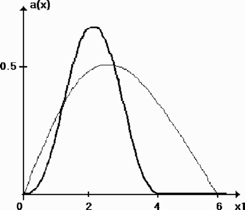
Figure 3. Test 1: the original function and the reconstruction a₁₆₀ (2, x₂ , 2). The level of noise δ = 0.01.

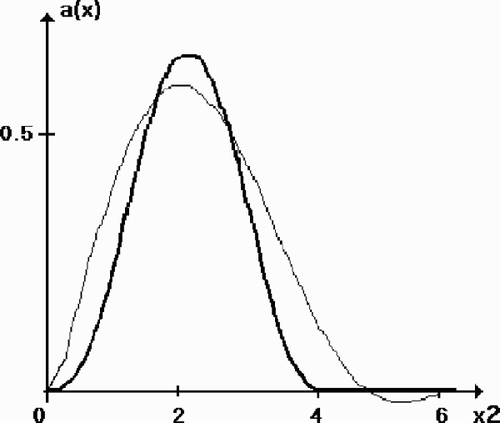
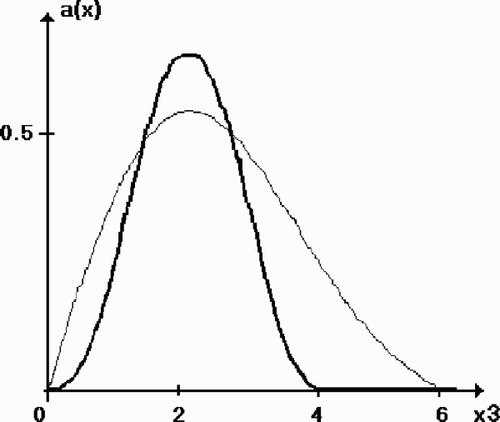
Figure 4. Test 1: the original function and the reconstruction a₁₆₀ (2, 2, x₃ ). The level of noise δ = 0.01.

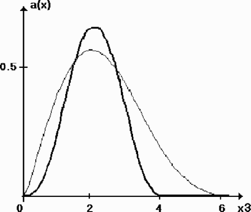
Test 2 In the second test we used the conjugate gradient method (20)(---203--20) , (23)(---203--23) , and (24)(---203--24) with (---203----118) . First, 40 iterations of the method were performed with δ = 0. We obtained r₄₀ = 0.04. In figure 5 the exact function (---203----119) (bold line) and the reconstructed function (---203----120) (thin line) are shown. Then, 40 iterations of the same process were performed with δ = 0.01. We obtained r₄₀ = 0.11. Figures 6–8 present the exact solution and the reconstructed functions (---203----121) ; (---203----122) , and (---203----123) obtained in the case of noisy data.

Figure 5. Test 2: the original function and the reconstruction . The level of noise δ = 0.

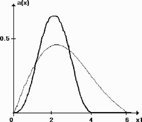
Figure 6. Test 2: the original function and the reconstruction . The level of noise δ = 0.01.

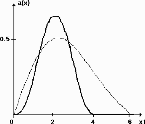
Figure 7. Test 2: the original function and the reconstruction . The level of noise δ = 0.01.

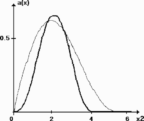
Figure 8. Test 2: the original function and the reconstruction . The level of noise δ = 0.01.

The analysis of figures 1–8 shows that the methods (19)(---203--19) and (20)(---203--20) give qualitatively good results in all the cases considered.

In [1,3,14]the interested reader will find several alternative solution methods for inverse medium scattering problems as well as results of corresponding computational experiments.

Acknowledgment

This work was supported by RFBR, project No 03–01–00352.