Optimal parameterization of a mathematical model for solving parameter estimation problems

Abstract

This article presents a method to solve parameter estimation problems by finding an optimal parameterization of the mathematical model. The pi-theorem of dimensional analysis is used to establish a formulation of the model based on dimensionless products and scaling parameters, together with the rules of a parameterization change. Logarithmic parameters are introduced for the purpose of working in a linear parameter space in which a given base corresponds to a specific parameterization. The optimal parameterization is assumed to yield uncorrelated estimators. A statistical independence criterion based on the Fisher information matrix is derived for maximum-likelihood estimators. The method allows one to solve inverse problems with highly correlated model parameters by identifying well-resolved parameters, leading to a solution expressed in terms of correlation laws between physical quantities.

Keywords:

• Dimensional analysis
• Fisher information
• Inverse problems
• Logarithmic parameters
• Optimal parameterization
• Parameter estimation
• Regularization

Introduction

Solving parameter estimation problems in science and engineering requires a mathematical model to describe the physical processes involved in an experiment [1, 2]. Generally speaking, the physical quantities of a model can be combined to form other physical quantities. For instance, in heat transfer, thermal conductivity and specific heat can be combined to obtain thermal diffusivity and effusivity. A change in the choice of the physical quantities should give exactly the same solution to the model. However, as Tarantola [2] and Vignaux [3] noted, each parameterization leads to a specific parameter estimation problem. For this reason, it is always useful to identify parameters whose estimation is a well-posed inverse problem satisfying existence, unicity and stability conditions. In many cases, scientists and engineers have a good idea about the significant parameters of their experiments. However, the task is not trivial when multiple physical quantities are involved and couple in complex manners. A number of difficult problems appear for instance in heat conduction and other irreversible phenomena [4] in which parameters are often highly correlated, leading to ill-posed inverse problems.

In this article, we propose a method aimed at identifying the optimal parameterization of a mathematical model for parameter estimation and data fitting. A parameterization is assumed to be optimal under the following conditions:

1.	the parameterization should be complete and minimal.
2.	the correlation coefficients between the parameter estimators should be minimal.

Condition (a) stipulates that the parameterization should include the minimal number of parameters needed to fully describe the physical processes involved. This condition can be fulfilled thanks to the well-known technique of dimensional analysis. This technique can lower the number of parameters in a model without loss of information [3,5]. Dimensional analysis provides complete and minimal sets of dimensionless quantities. A specific set corresponds to a base of a certain space, and a change of base allows a new set of parameters to be obtained. Condition (b) is closely related to the well-posed character of the inverse problem. It is a condition which guarantees the existence, unicity and stability of parameter estimators. A criterion based on Fisher information is used here to define minimal correlations and thereby the optimality of the parameterization. This criterion can be applied when the inverse problem is stated with the logarithms of dimensionless quantities as the model parameters. We emphasize the advantages of trading a set of physical parameters, possibly highly correlated, for a set of minimally correlated logarithmic parameters. The use of an optimal parameterization leads to a simple projection method to provide a regularized maximum-likelihood solution in both linear and nonlinear problems. Furthermore, we show that this solution reduces to a set of correlation laws between the physical parameters of the model.

In section 1, the pi-theorem of dimensional analysis is used to derive a method to explicitly formulate any mathematical model using dimensionless products, scaling parameters, explanatory and output variables. The pi-theorem is also applied to derive nonlinear relationships describing a change of parameterization. Logarithmic parameters are introduced to transform these relationships into a linear system. In section 2, the statistical criterion based on the Fisher information matrix is established. This criterion is applied to logarithmic parameters in order to define a new base of uncorrelated parameters. Section 3 presents a regularized maximum-likelihood solution of problems which are linear with respect to logarithmic parameters. In section 4, the regularized linear solution is used to build an iterative algorithm aimed at reaching the solution of general nonlinear problems. A simple example of the technique in the field of heat transfer is presented in section 5.

1. Model parameterization using dimensional analysis

The purpose of dimensional analysis is to determine relationships between parameters using only one assumption: physical laws are independent of arbitrarily chosen units of measure. As a consequence, physical equations must be homogeneous and can be expressed with dimensionless quantities, which are pure numbers. Let x ₁, x ₂, … , x _n be the n physical quantities of the problem. These quantities must involve w independent dimensions s _k of the employed system of units. The dimension of quantity x _i , noted [x _i ], can be expressed as products of powers of dimensions s _k :

where a _ki are real numbers. The dimensional matrix of the problem is defined as the w × n rectangular matrix M formed by numbers a _ki . The pi-theorem [6,7] states that the problem can be described by an implicit function of m dimensionless products π ₁, … , π _m , m being given by m = n − r, where r is the rank of the rectangular matrix M. The dimensionless products are defined from the physical quantities x _i by monomial expressions:

where b _ji are real numbers. The quantities π _j form a complete set of parameters for describing the physical problem. The pi-theorem does not give the values of numbers b _ji . Instead, it implies that the set of m vectors b _j  = (b _{j 1}, … , b _jn ) must be linearly independent and form a base of the nullspace of M [6]. equation (1) shows that a complete set of π _j , called a dimensionless parameterization, is defined by the m × n matrix B formed by coefficients b _ji .

According to the pi-theorem, the dimensionless form of a mathematical model function is an homogeneous function of parameters π _j . In order to use the function for data fitting and parameter estimation, an output variable is needed as well as an explanatory variable. The explanatory and output variables should explicitly appear as dimensional parameters in the model. Let us assume that the output variable is x ₁ and the explanatory variable is x ₂. In this case, the set of dimensionless products must be built to include two parameters π ₁ and π ₂, in which x ₁ and x ₂ appear separately. The model function can be formulated in the following form:

The remaining m − 2 model parameters π ₃…π _m have to be determined in order to complete the parameterization. A mathematical method to find dimensionless products, with constraints on the choice of one or several of them, is given in [7]. It consists in separating the set of dimensional quantities x _i into m quantities x ₁, … , x _m and n − m quantities x _{m +1}, … , x _n . After eliminating one or more linearly dependent rows in M, matrices M and B can be partitioned as [M ₁ | M ₂] and [B ₁ | B ₂]. B ₁ is a m × m matrix whose coefficients can be chosen to introduce ad hoc dimensionless products in the problem. The value of four coefficients of B ₁ can be set to define π ₁ and π ₂ as being respectively linear in x ₁ and x ₂: (B ₁)₁₁ = 1, (B ₁)₂₂ = 1, (B ₁)₁₂ = 0, (B ₁)₂₁ = 0. Submatrix B ₂ can be computed using the following relationship:

The resulting products π ₁ and π ₂ can be expressed as:

From equation (3), two scaling parameters X ₁ and X ₂ relative to x ₁ and x ₂ can be introduced:

Equations (3) can be rewritten in the following way:

Scaling parameters X ₁ and X ₂ have the reciprocal dimensions of x ₁ and x ₂ (inverse units). Now, the model can be explicitly formulated using dimensional variables x ₁ and x ₂, scaling parameters X ₁ and X ₂, and m − 2 dimensionless products π ₃ , … , π  _m . In order to preserve the dimensionless form of the model function, the scaling parameters X ₁ and X ₂ can be normalized by reference values (X ₁)_ref and (X ₂)_ref, leading to dimensionless scaling parameters

and

:

(X ₁)_ref and (X ₂)_ref can be set to any practical values, such as 1, expressed in inverse units of x ₁ and x ₂. The resulting model function is obtained from equation (2) by replacing π ₁ and π ₂ by x ₁, x ₂,

and

:

Scaling parameters

and

can be considered as model parameters too, leading to the more general form:

The minimal and complete set of m model parameters

constitutes a model parameterization associated with matrix B = [B ₁ B ₂] relative to (π₁,…,πm). Therefore, in the following sections, the formal distinction is no longer made between scaling parameters and quantities π _j . The dimensionless parameterization obtained by dimensional analysis will be simply referred to as (π₁,…,πm), even if this set includes dimensionless scaling parameters obtained by the procedure described in this section.

The implicit consequence of the pi-theorem is the existence of an infinite number of dimensionless parameterizations, each corresponding to a particular base of the nullspace of M. Given a dimensionless parameterization π _j associated with matrix B, another dimensionless parameterization π′ _j associated with a matrix B′ can be obtained through the following relationship:

where R is a non-singular m × m matrix. equation (5) can be expanded in the following form:

where coefficients r _jk are the elements of matrix R. Using the definitions of π _j and π′ _j as functions of x _i and equation (6), the following relationship is derived:

equation (7) defines the change from parameters π _j to parameters π′ _j . It represents a set of nonlinear relationships that can be transformed into a linear system by using the logarithm function. This operation is mathematically consistent because quantities π _j and π′ _j are dimensionless. Besides, if all physical quantities involved in the model are positive, π _j and

must be positive as well so that their logarithms always exist. Taking the logarithm on both sides of equation (7) gives:

Let us now define logarithmic parameters u_j = log(π _j ) and

. Parameters u _j and v _j can be put together in respective vectors u and v. equation (8) can then be written in vector–matrix notation as v = Ru. This relationship shows that linear combinations of log-parameters define other log-parameters. Therefore, logarithmic parameters belong to linear spaces. Linear algebra techniques [8] can be consequently applied in log-parameter spaces while they would be inconsistent in non-logarithmic parameter spaces. Other useful properties of log-parameters are detailed by Tarantola and Mosegaard in [9]. In particular, a logarithmic estimator associated with a Gaussian probability density function implies a log-normal probability density function for the corresponding non-logarithmic estimator. It is worth noting that the current guidelines for computing measurement uncertainties described in the ISO guide [10] emphasize using the Gaussian probability density. However, as Cox et al. note, this distribution only gives good results when uncertainties are small [11]. In many instances, a Gaussian estimator having small mean and large variance gives a confidence interval with meaningless negative values. As the log-normal distribution is only defined for positive variables, it eliminates negative values. As a consequence, estimators with arbitrary large variances can be consistently described. Being a non-symmetrically skewed distribution [2], the log-normal probability density function provides non-symmetrical confidence intervals.

2. The identification of uncorrelated parameters

The inverse problem is now defined as the problem of estimating a vector u of m log-parameters and finding the linear transformation which gives an optimal parameterization represented by parameter vector p. Let us assume a vector d of N measurement data corresponding to N values of the explanatory variable. The standard model relationship d = g(u) + ε is assumed, in which vector g(u) comprises N values of the nonlinear model function g given by equation (4) and ε is the vector formed by the N values of a zero-mean random noise. The maximum likelihood estimator

is obtained through the maximization of the likelihood probability density f(u). This estimator has well-known desirable features [1, 12]: it is a consistent estimator, at least asymptotically unbiased, asymptotically efficient and asymptotically distributed as a Gaussian random vector. Because of these properties, the covariance matrix C _u of

asymptotically equals the Cramér-Rao lower bound [12]:

where J _u is the Fisher information matrix:

equation (9) means that the covariance matrix tends towards the inverse Fisher information matrix when enough data are taken into account. By definition, an optimal parameterization gives minimally correlated estimators. This condition is reached when the Fisher information matrix is diagonal. In this case, the off-diagonal elements of the covariance matrix tend to zero, which ensures that the correlation coefficients are asymptotically null. Therefore, finding the optimal parameterization p is equivalent to finding a diagonal Fisher information matrix J _p .

From a mathematical point of view, the Fisher information matrix corresponds to a linear mapping from the parameter space to the dual space [2]. If a parameter space is subtended by a base consisting of n dimensional quantities, then the dual base comprises n quantities having reciprocal dimensions. When the parameter space is subtended by a base of logarithmic parameters, the dual base also consists of logarithmic parameters. A remarkable consequence is that the Fisher information matrix of logarithmic estimators maps the parameter space into itself. Under this condition, the eigenvector–eigenvalue decomposition [8, 13] of J _u can be performed, which leads to the relationship:

where Λis the diagonal matrix whose elements are the eigenvalues Λ _j of J _u . Matrix V is the m × m orthogonal matrix whose columns are the eigenvectors of J _u . The Fisher information matrix being symmetric and positive definite, the eigenvalues Λ _j are always positive and the eigenvectors are always present to the full number m [13]. Matrix V defines a new base of the log-parameter space in which the Fisher information matrix is diagonal. Therefore, the parameterization p given by the following equation is optimal:

The optimal parameters p _j of the problem are completely defined by equation (10). The Fisher information of each estimator

is equal to Λ _j . According to the Cramér-Rao lower bound, the minimal variance of

is:

It is interesting to note that the variance of a logarithmic random variable log(x) can be expressed as a function of the variance of the non-logarithmic random variable x:

The variance of a logarithmic estimator can be seen as the square of a relative uncertainty, which is dimensionless. In turn, the Fisher information Λ _j can be seen, through equation (11), as the inverse of a squared relative uncertainty.

When the initial log-parameters u _j are highly correlated, the complete set cannot be simultaneously estimated. Since a parameterization change does not modify the amount of information, the set of optimal parameters p _j cannot be simultaneously estimated. However, the set of m parameters p _j can be divided into two subsets of parameters according to the amount of Fisher information they possess:

1.	s parameters : badly-resolved or unresolved parameters corresponding to small or null Fisher information.
2.	m − s parameters : well-resolved parameters corresponding to large Fisher information.

In the case of logarithmic parameters, the lowest significant value of Fisher information may be set to 1, which according to equation (11), corresponds to a maximal relative uncertainty of 100%. In real problems, the “cut-off” point can be set to a different value, provided matrix Λ ⁺ remains sufficiently well-conditioned for numerical application. The parameter estimation problem can be projected in the subspace of the m − s well-resolved parameters

, leading to a well-posed inverse problem of smaller dimension than the original problem. The projected Fisher information matrix Λ ⁺ is obtained from Λ by simply suppressing the rows and columns corresponding to parameters

.

The techniques consisting of suppressing small eigenvalues for solving underdetermined problems are well-known [13]. They define a class of regularization methods which eliminates numerical instabilities by improving the conditioning of matrices. The method described here has the same advantage. The suppression of a number s of small eigenvalues Λ _j transforms an ill-posed problem of dimension m into a well-posed problem of dimension m − s. Moreover, this procedure is based on consistent mathematical operations and leads to the identification of physically meaningful parameters. The number s can be seen as the degeneracy number of the model, corresponding to the number of parameters that cannot be estimated by data inversion. The number m − s is the true dimension of the inverse problem, corresponding to the effective number of parameters that can be estimated.

It is straightforward to remark that the estimation of m − s well-resolved parameters

does not allow individual estimates of m log-parameters u _j to be obtained. However,

can be expressed as functions of u _j using equation (10) with the numerical values of the coefficients of the orthogonal matrix V. In turn, parameters π _j can also be introduced by applying the exponential function. The following m − s relationships are deduced:

Using equation (1), it is also possible to replace π _j by x _i using the coefficients of matrix B given by dimensional analysis. Equation (12) becomes:

Equation (12) represents a set of m − s correlation laws between dimensionless parameters π _j . Similarly, equation (13) is a set of m − s correlation laws between the physical quantities x _i . It is interesting to note that the exponent of x _i in the jth correlation law (equation 13) is the quantity

, which associates matrix B of dimensional analysis and matrix V obtained from the eigenvectors of the Fisher information matrix. These correlation laws faithfully represent all the information on the physical parameters given by the resolution of the inverse problem. Equation (13) can be seen as the mathematical representation of the coupling that occurs between the physical parameters x _i . No further information can be obtained on the value of the individual parameters under the stated assumptions. Figure 1 gives an overall view of the technique.

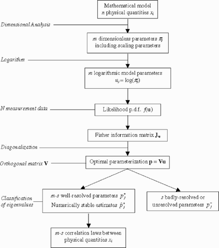
Figure 1. Schematic summary of the principles leading to the identification of an optimal parameterization of the mathematical model and the estimation of well-resolved parameters.

3. The Gaussian linear case

In the presence of Gaussian noise in the data, the maximum-likelihood estimator û is obtained by minimization of the well-known L₂-norm S _ML [1, 2]:

In this case, the Fisher information matrix is the Hessian of S _ML [1, 2]:

In this work, linearity relates to logarithmic parameters u _j . That is to say, a model function is linear if the output variable is a linear function of the logarithmic model parameters. The model function g(u) reduces to G _u u where G _u is the model matrix. The expression of the Fisher information matrix becomes:

The maximum-likelihood estimator

corresponding to the minimum of S _ML is given by:

The covariance matrix of û is

. An important consequence of equation (14) is that the Fisher information matrix does not depend on the actual estimate of u. The optimal parameterization can thus be determined by the direct diagonalization of J _u , giving the orthogonal matrix V. The model matrix G _p relative to the optimal parameters is given by the linear relationship:

Vector u can be replaced by V ⁻¹ p in equation (15) to obtain the expression of the maximum likelihood estimator

:

When all the parameters p are well-resolved, their diagonal covariance matrix C_p is given by C_p = Λ ⁻¹. Let us now suppose that the model matrix G _u shows approximate or exact linear dependencies between its columns. As a result, J _u becomes a poorly conditioned or singular matrix. This case is typical of ill-posed inverse problems leading to high correlation coefficients between the parameters. The inverse of J _u is either highly unstable or undefined [13]. Matrices J _u and Λ being mathematically similar, Λ has the same condition number as J _u . As a consequence, the estimator

given by equation (17) cannot be reliably computed. Nevertheless, according to the methodology described in the previous section, it is possible to solve the inverse problem in the subspace of the m − s well-resolved parameters

corresponding to the large eigenvalues of Λ. The orthogonal projection G _p ⁺ is obtained from G _p by suppressing the s columns corresponding to the rejected parameters. The remaining m − s parameters can be put together in a vector p ⁺ . The maximum-likelihood estimator of p ⁺ can then be expressed as:

The covariance matrix

of

is:

Equations (18) and (19) provide a regularized solution to the linear parameter estimation problem. As shown in section 2, this solution reduces to a set of correlation laws when the exponential of

is taken. Variable

being a Gaussian variable,

is a log-normal variable, associated with a non-symmetrical confidence interval that can be expressed with the following bounds:

where cf is a coverage factor determined from the Student distribution according to the desired confidence level and the number of degrees of freedom of the problem [1, 2]. In this case, the latter is equal to N − (m − s).

4. The Gaussian nonlinear case

In nonlinear problems, the model function g is not linear with respect to the logarithmic model parameters u _j . As a consequence, the mimimum of the L₂-norm S _ML has to be determined by a numerical procedure. In this case, finding the optimal parameterization is not straightforward because the Fisher information matrix depends on the actual estimates of the model parameters. Nonetheless, a linearized approach can be used to determine the optimal parameterization and to minimize S _ML by proceeding step by step from initial guess values of the parameters. The linearization of the model must be performed with respect to log-parameters in order to apply the methodology and formulas of the previous sections. The first order Taylor expansion of g(u) around a reference parameter vector u _r gives:

where

is a Jacobian matrix, known as the sensitivity matrix, defined by:

where (x ₁) _i is the ith value of the explanatory variable x ₁. The local Fisher information matrix

can be calculated using equation (14) previously established in the linear case. The optimal parameterization p _r corresponding to the linearized problem is now given the eigenvalue–eigenvector decomposition of

, providing an orthogonal matrix V _r and a diagonal Fisher information matrix Λ _r:

In the context of the numerical minimization of S _ML, the parameterization of the problem can be adaptively changed using equation (23), while an iterative algorithm proceeds to find a minimum. This is particularly useful in the case of local minimization techniques, such as the Gauss-Newton method, relying on the explicit computations of the gradient and the Hessian. The change of parameterization defines, at each step, a subspace of well-resolved parameters. In this way, numerical instabilities caused by correlated parameters are automatically avoided. The computation of the mathematical model is made possible at each step by using the total orthogonal matrix W corresponding to the change of the initial parameterization u to the current optimal parameterization p. Matrix W is the left product of the successive orthogonal matrices V obtained at each step:

A minimization technique can be implemented in the following way:

1.	Apply dimensional analysis to the model and introduce parameterization u formed by m logarithmic parameters u j .
2.	Define first guess values u 0
3.	Set initial orthogonal matrix W 0 to I (m × m identity matrix)
4.	Compute model g(u k )
5.	Compute cost function
6.	Compute sensitivity matrix by differentiation of the model function g(u k )
7.	Compute Fisher information matrix:
8.	Perform eigenvector–eigenvalue decomposition: with 1. Orthogonal matrix V k 2. Diagonal Fisher information matrix
9.	Define optimal parameters: p k = V k u k
10.	Compute new sensitivity matrix:
11.	Compute total orthogonal matrix:
12.	Partition vector p k with respect to Fisher information: 1. Well-resolved parameters 2. Badly-resolved parameters
13.	Update value of well-resolved parameters by the Gauss-Newton step:
14.	Leave value of badly-resolved parameters unchanged
15.	Define new set of parameters:
16.	Check convergence. Three conditions must be simultaneously fulfilled: 1. S ML reaches a minimum 2. Gauss-Newton step tends to the null vector 3. Orthogonal matrix V k tends to the m × m identity matrix
17.	If convergence is not reached, increment k and go to step 4

When the three convergence tests are satisfied, the algorithm provides the maximum-likelihood estimate

of the optimal parameters, the diagonal Fisher information matrix J _p and an orthogonal matrix W. As usual in parameter estimation, the goodness of fit can be checked by comparing the minimum value of S _ML to tabulated chi-squared values.

When all the parameters of vector p are well-resolved, their diagonal covariance matrix C _p can be directly computed by

. The orthogonal matrix W can be used to transform the estimates

into estimates û by the relationship

. The covariance matrix C _u is then given by C_u = W ⁻¹ C_p W. Like in the linear case, the initial problem of estimating m correlated parameters u may lead to the estimation of a reduced number m − s of well-resolved independent parameters p ⁺. The solution of the inverse problem is a set of m − s correlation laws, which can be expressed from the maximum-likelihood estimates

and the coefficients of matrix W using the methodology presented in section 2.

The proposed iterative algorithm is able to deal with highly correlated parameters and ensures convergence to the maximum-likelihood point under the following conditions:

1.	The mathematical model must be accurate enough to fit the data.
2.	The model function must be differentiable in order to compute the sensitivity and Fisher information matrices.
3.	The model function should not be highly nonlinear to ensure validity of the linearized equation (21) at each step.
4.	Initial guess values should not be too far from maximum-likelihood point (condition resulting from the use of a local minimization technique). Trying multiple starting points is often necessary to find a solution and check its unicity.
5.	Absence of outliers in the data (condition resulting from the Gaussian hypothesis and the use of the corresponding L2-norm).

In comparison with the standard Gauss-Newton method, the extra computational cost is the storage of the orthogonal matrices V _k and W _k . Moreover, the time required to perform the diagonalization of the Fisher information matrix makes this method slower. Nonetheless, this algorithm cannot fail, even in the presence of perfect correlations between two or more parameters.

5. Example

This section provides an example illustrating the benefits of using an optimal parameterization in a parameter estimation problem of small dimension. The problem consists in measuring thermal properties of titanium nitride (TiN) coatings on steel substrates using photothermal radiometry [14, 15]. The coating is heated by a modulated continuous-wave laser beam in order to produce a harmonic temperature field in the sample. An infrared radiometer with a lock-in amplifier provides the amplitude and phase of the surface temperature [14]. The phase ϕ is used for parameter estimation and data fitting. It is measured at different modulation frequencies f in the range of 1 kHz–1 MHz, which gives thermal diffusion lengths varying from about 100 µm to 3 µm, the latter value corresponding to the approximate thickness of the coating. The coating is opaque at the excitation and detection wavelengths. In the experimental configuration of [14], the heat conduction regime is one-dimensional. The surface temperature is modeled using thermal quadrupoles assuming a homogeneous coating, a semi-infinite substrate and a thermal resistance at the interface. The phase ϕ is given by the argument of the complex thermal impedance [14]:

with γ being the thermal diffusion constant:

In equations (24) and (25), R is the thermal resistance of the interface, e _∞ is the thermal effusivity of the substrate, λ is the thermal conductivity of the coating, L is the thickness of the coating, D is the thermal diffusivity of the coating and i is the imaginary number

. Figure 2 illustrates the dimensional analysis of the model. A minimal and complete set of three model parameters is obtained:

Figure 2. Dimensional analysis of the model function given by equation (24). One row of matrix M has to be rejected because the rank of M is equal to 3 while there are four fundamental units. The row corresponding to the Kelvin unit can be rejected because it is proportional to the row corresponding to the kilogram unit. As described in section 1, matrices M and B are partioned in order to introduce products π ₁ and π ₂ depending linearly on explanatory variable f and output variable ϕ. This is achieved here by setting submatrix B ₁ to the identity matrix. Submatrix B ₂ is given by B ₂ = − B ₁(M ₂ ⁻¹ M ₁)^t.

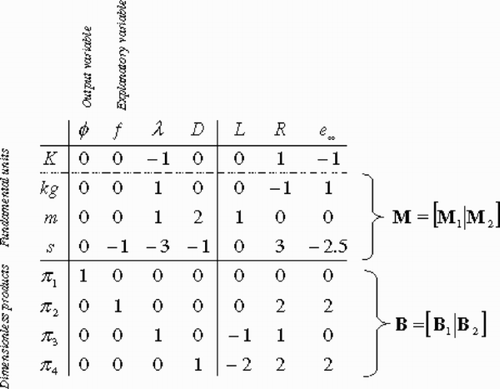
1.	Scaling parameter , relative to the explanatory variable f
2.	Dimensionless parameter π3 = λR/L
3.	Dimensionless parameter

Let us assume that the experiment gives a set of N = 100 logarithmically spaced data points in the 1 kHz–1 MHz frequency range. For simplicity, it is also assumed that the data points are mutually independent and that the phase data are associated with a uniform Gaussian noise of standard deviation equal to 1°. The covariance matrix C _d of the data (measured in degree) is therefore the identity matrix. The maximum-likelihood estimation of X ₂, π₃ and π₄ from the set of data is a nonlinear inverse problem.

5.1. Sensitivity and expected correlation coefficients

The model parameters are now set to typical values corresponding to the properties of a TiN coating on a steel substrate: λ = 10 K⁻¹ kg m s⁻³, D = 3.6 × 10⁻⁶ m² s⁻¹, L = 3 × 10⁻⁶ m, R = 6 × 10⁻⁸ K kg⁻¹ s³, e _∞ = 7000 K⁻¹ kg s^−5/2. The value of the scaling parameter X ₂ is 0.176 μs. The dimensionless scaling parameter

is obtained by normalizing X ₂ by a reference value of 1 μs. The values of the dimensionless parameters are :

 = 0.176, π₃ = 0.2 and π₄ = 0.0706. The ill-posed character of the parameter estimation problem can now be studied around these reference values by computing the sensitivity matrix G given by equation (22) and the Fisher information matrix J = 

. All the computations presented in this section were carried out on a standard PC using the scientific software Scilab (#INRIA-ENPC). Four parameterizations are first considered:

1.	Dimensional parameters λ, D, L, R and e ∞.
2.	Logarithms of dimensional parameters: log(λ), log(D), log(L), log(R) and log(e ∞).
3.	Dimensionless parameters , π3 and π4.
4.	Logarithmic parameters log( ), log(π3) and log(π4).

Table 1 gives the condition number of the Fisher information matrix in each case and the expected correlation coefficients between the estimators obtained by inverting the Fisher information matrix and normalizing the elements of the resulting covariance matrix.

Table 1. Condition number and expected correlation coefficients associated with several non-optimal parameterizations of the example in section 5.

Parameterization	Condition number of J	Expected correlation coefficients
1	× 10^30	Not computed, J numerically singular
2	2 × 10^13	−0.57 ; −0.57 ; −0.991 ; 0.991
		0.999 ; 0.68 ; −0.68 ; −0.68; −0.999
3	5 × 10^3	0.96 ; 0.97 ; 0.999
4	4 × 10^3	0.96 ; 0.97 ; 0.999

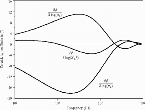
In the first case, the very high condition number of the Fisher information matrix shows that the estimation of the five dimensional parameters is an ill-posed inverse problem that cannot be solved directly. The use of logarithms of dimensional quantities in the second case improves the conditioning of the matrix. However, high correlation coefficients are present between the estimators. The dimensionless parameter set of the third case corresponds to a problem of smaller dimension but also exhibits high correlation coefficients. In the fourth case, the use of logarithmic parameters does not reduce the correlation coefficients. These four parameterizations lead to badly conditioned matrices and high correlation coefficients. None is really adapted to solve the parameter estimation problem. Figure 3 shows a plot of the sensitivity coefficients of the phase ϕ to the logarithmic parameters log(

), log(π₃) and log(π₄). This graph indicates that these three parameters have a significant influence on the output variable.

Figure 3. Sensitivity coefficients of the phase ϕ to the logarithmic parameters log(), log(π₃) and log(π₄).

An optimal parameterization is obtained by the diagonalization of the Fisher information matrix corresponding to the logarithmic parameterization of the fourth case. The resulting orthogonal matrix is:

where the coefficients are rounded off to the second decimal. The eigenvalues are Λ₁ = 19 566, Λ₂ = 348 and Λ₃ = 5. Matrix V defines a set of three optimal parameters p ₁, p ₂ and p ₃ as linear combinations of log(

), log(π₃) and log(π₄):

The optimal parameters are associated with Fisher informations Λ₁, Λ₂ and Λ₃. Parameters p ₁ and p ₂ are associated with a high Fisher information. They are the well-resolved parameters of the problem. Figure 4 shows a plot of the sensitivity of the phase to the optimal parameters, computed using equation (16). It is worth noting that the three curves are linearly independent. Besides, the sensitivity to the parameter p ₃ is below the noise level of 1°. With a small Fisher information, parameter p ₃ is a badly-resolved parameter.

Figure 4. Sensitivity coefficients of the phase ϕ to the optimal parameters p ₁, p ₂ and p ₃.

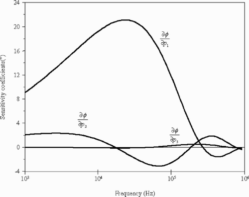
Now, the parameter estimation problem can be solved with respect to well-resolved parameters p ₁ and p ₂. The condition number of the projected 2 × 2 diagonal Fisher information matrix Λ ⁺ is about 60. This value is much smaller than the initial condition numbers obtained with non-optimal parameterizations. It improves the stability of the inverse problem near the reference values.

5.2. Assessment of the iterative algorithm with simulated data

The efficiency of the algorithm given in the previous section can be verified by using simulated data. In this example, a set of theoretical data are obtained using equation (24) with the reference numerical values used above. A random noise with a standard deviation of 1° is added to the data. The chosen initial values of parameters X ₂, π₃ and π₄ differ from the true values by about one order of magnitude or less: (

)₀ = 0.01, (π₃)₀ = 1 and (π₄)₀ = 0.1. As expected, the standard Gauss-Newton algorithm with parameterizations (

, π₃, π₄) or (log(

), log(π₃), log(π₄)) systematically fails because of the bad conditioning of the matrices. On the contrary, the algorithm based on optimal parameters converges after six iterations. The numerical results obtained after each iteration are listed in Table 2.

Table 2. Results given by the iterative algorithm applied to the example in section 5.

k	V k	Λ k	p k	δp k	S ML
1		Λ1 = 20035	p 1 = − 0.534	δp 1 = 0.996	20807
		Λ2 = 0.1	p 2 = −4.765	δp 3 = 0.935
		Λ3 = 553	p 3 = −1.876
2		Λ1 = 19116	p 1 = −0.226	δp 1 = 0.01	1055
		Λ2 = 187	p 2 = −2.490	δp 2 = 1.00
		Λ3 = 0.33	p 3 = 4.190
3		Λ1 = 20754	p 1 = −0.160	δp 1 = −0.03	525
		Λ2 = 9.69	p 2 = −4.218	δp 2 = −1.37
		Λ3 = 144.6	p 3 = 1.400
4		Λ1 = 19152	p 1 = −0.190	δp 1 = −0.03	136
		Λ2 = 263	p 2 = −0.257	δp 2 = −0.07
		Λ3 = 2.58	p 3 = 4.210
5		Λ1 = 19264	p 1 = −0.220	δp 1 = 0.0003	115.6
		Λ2 = 324	p 2 = 0.215	δp 2 = −0.017
		Λ3 = 2.16	p 3 = 4.208
6		Λ1 = 19233	p 1 = −0.220	δp 1 = 0	115.5
		Λ2 = 324	p 2 = 0.234	δp 2 = 0
		Λ3 = 2.12	p 3 = 4.208
Total orthogonal matrix

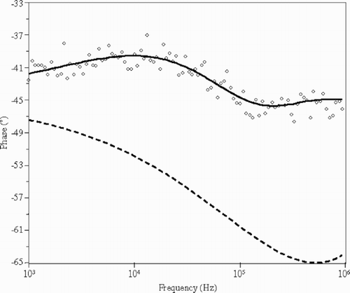
At each step, one badly-resolved parameter is rejected and the Gauss-Newton correction acts on two optimal parameters. The orthogonal matrix V ₆ obtained after convergence is equal to the identity matrix (in absolute value). The total orthogonal matrix W defines the optimal parameters of the inverse problem. The absolute values of coefficients of matrix W are very close to the coefficients of the matrix V previously computed from the sensitivity coefficients at the reference values. Since the signs of the coefficients of the orthogonal matrices are not constrained, equivalent optimal parameters with opposite values may be obtained. Figure 5 shows the simulated data, the data corresponding to the initial values and the data corresponding to the maximum-likelihood model.

Figure 5. Graph showing the simulated phase data (dots), the data corresponding to the initial parameter values of the iterative algorithm (dashed line) and the best fit data obtained after convergence of the iterative algorithm (plain line).

The maximum-likelihood estimates of the optimal parameters are p ₁ = −0.220, p ₂ = 0.233, p ₃ = 4.208. The variances and standard deviations can be computed from the Fisher information values using equation (11): σ(p ₁) = 0.0016, σ(p ₂) = 0.013 and σ(p ₃) = 2.89. According to equation (13), the estimation of well-resolved parameters p ₁ and p ₂ provides the following correlations laws between the physical parameters:

The constants (10⁶)^0.05 and (10⁶)^0.837 come from the normalizing value of 10⁻⁶ s in the dimensionless scaling parameter

. The confidence intervals of exp(p ₁) and exp(p ₂) are computed from equation (20), in which a coverage factor of 2 is used:

Estimates of the initial log-parameters can be computed using relationship u = W ⁻¹ p: log(

) = −2.11, log(π₃) = −1.86 and log(π₄) = −3.148. The covariance matrix C _u of these estimates can be computed using relationship C_u = W ⁻¹ ΛW. The obtained standard deviations on the log-parameter estimates are respectively σ(log(

)) = 0.38, σ(log(π₃))=0.26 and σ(log(π₄))=0.51. By using the exponential function, estimates of the original dimensionless parameters of the problem can be obtained:

 = 0.1213, π₃ = 0.156, π₄ = 0.043. The associated confidence intervals computed with a coverage factor of 2 are:

The obtained confidence intervals are quite large, which is not surprising given the high correlation coefficients between these parameters.

Using the optimal parameters and their maximum-likelihood estimates, all the other dimensionless parameters of the problem can be estimated. For instance, the logarithmic thermal effusivity ratio between the coating and the substrate, equal to

, and its variance can be derived:

with

Conclusion

This article demonstrates that parameter estimation problems can be solved using an optimal parameterization consisting of uncorrelated parameters. These parameters are determined by the diagonalization of the Fisher information matrix relative to logarithmic estimators. This work relies on dimensional analysis to provide minimal and complete sets of dimensionless model parameters, associated with rules for describing parameterization changes. As a result, an initial set of correlated parameters can be transformed into a set of optimal parameters, allowing a reduced number of well-resolved parameters to be identified. The estimates of these well-resolved parameters lead to a solution of the inverse problem expressed as a set of correlation laws between physical quantities.

This method was detailed for maximum-likelihood estimation problems under the Gaussian noise hypothesis. In the linear case, the optimal parameters can be determined directly from the model matrix and the covariance matrix of the data. In the case of nonlinear problems, the optimal parameterization can be determined by an iterative algorithm aimed to minimize the L₂-norm of the problem in the subspace of well-resolved parameters. This algorithm has the property of being numerically stable, in the case of high or perfect correlations between the initial parameters.

In this work, the optimal parameters are defined as being uncorrelated. Null correlation coefficients assure the mutual independence of the parameters up to the second order, which is well adapted to Gaussian estimators. However, this criterion is not sufficient to ensure the statistical independence of non-Gaussian estimators. Higher order criteria, commonly used in the independent component analysis [16], could greatly improve the method in the case of non-Gaussian distributions, appearing in many nonlinear inverse problems.

The technique presented in this article was applied in the field of thermal metrology to the characterization of hard coatings by photothermal infrared radiometry [14, 15]. The complete experimental results will be the subject of a different paper. The estimation of scaling parameters such as defined in section 1 of this article, is presented in [17] and led to the measurement of the thermal diffusivity of semi-infinite solids.

Acknowledgements

I am grateful to Prof. Albert Tarantola of the Institut de Physique du Globe de Paris, France, for helpful comments made to the early version of this work. I acknowledge stimulating discussions with Dr. Gordon Edwards of the National Physical Laboratory, Teddington, UK. I would also like to thank Prof. Pierre Trebbia of the University of Reims, France, for his graduate course on multivariate statistics and his incentive to use Fisher information in Physics.

Nomenclature

Table

Superscripts:
+	=  Relative to well-resolved parameters
−	=  Relative to badly-resolved parameters
⁁	=  Maximum-likelihood estimators
t	=  Transposed matrix
Subscripts:
r	=  Relative to reference values
k	=  Relative to the kth iteration of nonlinear algorithm
Scalars:
Roman symbols:
a ki	=  Dimensional exponents of x i
b ji	=  Exponents of dimensionless products π j
	=  Exponents of dimensionless products
cf	=  Coverage factor used for computing confidence intervals
D	=  Thermal diffusivity of coating
e ∞	=  Thermal effusivity of substrate
f	=  Modulation frequency
F(.)	=  Implicit function of dimensionless product
f(u)	=  Likelihood probability density function
g(.)	=  Individual value of model function g
i, i′, j, j′, k	=  Indices
L	=  Thickness of coating
m	=  Number of dimensionless products
n	=  Number of physical quantities
N	=  Number of measurement data
p j	=  Optimal parameters
R	=  Thermal resistance of interface
r jk	=  Elements of matrix R
r	=  Rank of matrix M
s	=  Number of badly-resolved parameters
s k	=  Fundamental dimensions of the chosen system of units
S ML	=  Maximum-likelihood cost function
u j , v j	=  Logarithmic parameters
V jk	=  Elements of matrix V
w	=  Number of independent dimensions
X 1, X 2	=  Scaling parameters
,	=  Dimensionless scaling parameters
x i	=  Physical quantities of mathematical model
Greek symbols:
π j ,	=  Dimensionless products
Λ j	=  Fisher information of p j
ϕ	=  Phase of surface temperature
γ	=  Harmonic thermal diffusion constant
λ	=  Thermal conductivity of coating
σ	=  Standard deviation
Vectors:
Roman symbols:
b j	=  Vector of elements (b j 1,…,b jn )
d	=  Vector of N measurement data
g(u)	=  Vector of N values of model function g
p	=  Vector of optimal parameters
u, v	=  Vectors of logarithmic parameters
Greek symbols
ε	=  Vector of N values of a Gaussian random noise
δp k	=  Gauss-Newton correction in nonlinear iterative algorithm
Matrices:
Roman symbols:
B	=  Matrix of elements b ji
B′	=  Matrix of elements
C d	=  Covariance matrix of measurement data vector d
C u	=  Covariance matrix of maximum-likelihood estimate of u
C p	=  Covariance matrix of maximum-likelihood estimate of p
G u	=  Model matrix or sensitivity matrix with respect to log-parameters u j
G p	=  Model matrix or sensitivity matrix with respect to optimal parameters p j
I	=  Identity matrix
J u	=  Fisher information matrix relative to u
J p	=  Fisher information matrix relative to p
M	=  Matrix of elements a ki
R	=  Non-singular m × m matrix
V	=  Orthogonal matrix
W	=  Total orthogonal matrix
Greek symbols:
Λ	=  Diagonal Fisher information matrix

References

- Beck JV Arnold KJ 1977 Parameter Estimation in Engineering and Science New York J. Wiley & Sons
- Tarantola A 1987 Inverse Problem Theory, Methods for Data Fitting and Model Parameter Estimation New York Elsevier Science
- Vignaux GA 1992 Dimensional analysis in data modelling C.R. Smith, G.J. Erickson, and P.O. Neudorfer (Eds) Maximum Entropy and Bayesian Methods Dordrecht Kluwer Academic Publishers www https://www.mcs.vuw.ac.nz/~vignaux/diman.html
- Beck JV Blackwell B St Clair Jr CR 1985 Inverse Heat Conduction. Ill-posed Problems New York J. Wiley & Sons
- Kokar , MM . 1979 . The use of dimensional analysis for choosing parameters describing a physical phenomenon . Bulletin de l'Academie Polonaise des Sciences: Série des Sciences Techniques , XXVII ( 5/6 ) : 249
- Palacios J 1960 L’Analyse Dimensionelle Paris Gauthiers-Villars
- Szirtes T 1998 Applied Dimensional Analysis and Modeling New-York McGraw-Hill
- Mostow GD Sampson JH Meyer JP 1963 Fundamental Structures of Algebra New York McGraw-Hill
- Mosegaard K Tarantola A 2002 Probabilistic approach to inverse problems. In: International Handbook of Earthquake and Engineering Seismology Academic Press for the International Association of Seismology and Physics of the Earth Interior., www http://www.ccr.jussieu.fr/tarantola
- International Organization of Standardization (ISO) 1993 Guide to the Expression of Uncertainty in Measurement Switzerland Geneva
- Cox MG Dainton MP Harris PM 2001 Software Support for Metrology Best Practice Guide No. 6: Uncertainty and Statistical Modelling Technical report, National Physical Laboratory Teddington, UK www http://www.npl.co.uk/ssfm
- Van Trees HL 1968 Detection, Estimation and Modulation Theory New York J. Wiley & Sons
- Lanczos C 1961 Linear Differential Operators London D. Van Nostrand Company
- Martinsons , C and Heuret , M . 1999 . Inverse analysis for the measurement of thermal properties of hard coatings . High Temp. High Press. , 31 : 99
- Martinsons , C , Levick , A and Edwards , G . 2003 . Measurement of the thermal diffusivity of solids with an improved accuracy . Int. J. Thermophysics , 24 : 1171
- Hyuvärinen A Karhunen J Oja E 2001 Independent Component Analysis New York J. Wiley & Sons
- Levick , A , Lobato , K and Edwards , G . 2003 . Development of the laser absorption radiation thermometry technique to measure thermal diffusivity in addition to temperature . Rev. Sci. Instrum. , 74 : 612