Symbulate: Simulation in the Language of Probability

Abstract

Simulation is an effective tool for analyzing probability models as well as for facilitating understanding of concepts in probability and statistics. Unfortunately, implementing a simulation from scratch often requires users to think about programming issues that are not relevant to the simulation itself. We have developed a Python package called Symbulate (https://github.com/dlsun/symbulate) which provides a user friendly framework for conducting simulations involving probability models. The syntax of Symbulate reflects the “language of probability” and makes it intuitive to specify, run, analyze, and visualize the results of a simulation. Moreover, Symbulate’s consistency with the mathematics of probability reinforces understanding of probabilistic concepts. Symbulate can be used in introductory through graduate courses, with a wide variety of probability concepts and problems, including: probability spaces; events; discrete and continuous random variables; joint, conditional, and marginal distributions; stochastic processes; discrete- and continuous-time Markov chains; Poisson processes; and Gaussian processes, including Brownian motion. In this work, we demonstrate Symbulate, discuss its main pedagogical features, present examples of Symbulate graphics, and share some of our experiences using Symbulate in courses.

Keywords:

• Multivariate thinking
• Probability
• Random variables
• Simulation
• Stochastic processes
• Visualizing distributions

1 Introduction

Simulation can play a significant role in enhancing students’ ability to study random processes (Garfield and Ben-Zvi 2007) and understand probabilistic concepts. Simulations can be conducted by writing programs (in languages such as R, Python, or Matlab) or by using applets (Siegrist 2017; Dinov et al. 2016; Kahle 2014; Rossman and Chance 2017). But both options suffer from pedagogical limitations. Implementing a simulation from scratch in a language like R requires users to think about programming issues that are not relevant to the simulation itself, such as loops, vectorization, and commands for producing and customizing graphics. At the other extreme, applets require no programming but enable only a limited range of possible simulations.

We have developed a Python package called Symbulate which provides a user-friendly framework for conducting simulations involving probability models. Although simulations generally enhance the teaching and learning of probability, there are several ways that Symbulate goes beyond other methods of simulation, pedagogically and technologically:

1. Symbulate syntax reflects the “language of probability” and should be natural to anyone learning or familiar with probability. Symbulate syntax makes it intuitive to specify, run, analyze, and visualize the results of a simulation.

2. Symbulate commands and functionality are consistent with the mathematics of probability, which facilitates and reinforces understanding of probabilistic concepts.

3. Conducting and analyzing simulations in Symbulate requires minimal programming. Little to no previous experience with programming is needed to use Symbulate.

4. Symbulate enables easy and effective visualization of simulation output and probability distributions.

5. Symbulate can be used in introductory through graduate courses, with a wide variety of probability concepts and problems, including: probability spaces; events; discrete and continuous random variables; joint, conditional, and marginal distributions; stochastic processes; discrete- and continuous-time Markov chains; Poisson processes; and Gaussian processes, including Brownian motion.

6. Symbulate is fully compatible with Jupyter notebooks, which provide a user-friendly interface supporting interactive and reproducible programming and documentation.

In short, Symbulate programs are easy to write and run, and produce effective visualizations. The result is an environment where students can readily employ simulation to analyze virtually every probability problem.

In this work, we demonstrate the Symbulate package and discuss its main pedagogical features. We present various examples of Symbulate code and graphics. We provide comparisons between Symbulate and R, and discuss the advantages of Symbulate over other software packages and applets. We also share some of our experiences using Symbulate in courses.

2 Simulation in the Language of Probability

The syntax of Symbulate mirrors the “language of probability” in that the primary objects in Symbulate are the same as the primary components of a probability model:

1. a probability space consisting of the sample space (Ω) of possible outcomes ($\omega \in \Omega$) and a probability measure (P),

2. random variables (functions $X:\Omega \mapsto \mathbb{R}$) or stochastic processes (functions $X:T\times \Omega \mapsto \mathbb{R}$ for a (time) index set T) defined on the probability space, possibly via transformations of random variables or processes, and

3. related events (subsets $A\subset \Omega$ for which P(A) is defined), and in particular, conditioning on events.

Once these components are specified, Symbulate allows users to simulate many times from the probability model and summarize those results.

Symbulate commands complement the basic terminology and notation of probability, and should be intuitive to anyone learning or familiar with the subject. Moreover, Symbulate objects are consistent with the underlying mathematical objects. In this section, we introduce the Symbulate package and illustrate several ways in which the Symbulate syntax itself facilitates understanding of probabilistic concepts, in addition to simplifying programming of simulations and enabling easy and effective visualization.

Instructions for installing Symbulate can be found on the Github repository https://github.com/dlsun/symbulate. The following command imports Symbulate during a Python session.

from symbulate import *

Throughout this paper, code and output is displayed in the style of a Jupyter notebook, in which code cells are followed by any output they produce (Out[]:).

2.1 Probability Spaces and Random Variables

We introduce some of the core Symbulate commands with a simple example. Let X be the sum of two rolls of a fair four-sided die, and let Y be the larger of the two rolls (or the common value if a tie). The following Symbulate code defines a probability space P for simulating the 16 equally likely ordered pairs of rolls. The probability space in many elementary situations can be defined via a “box model.”

P = BoxModel([1, 2, 3, 4], size = 2, replace = True)

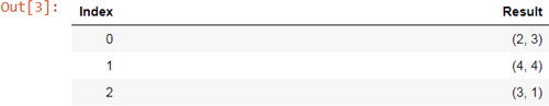
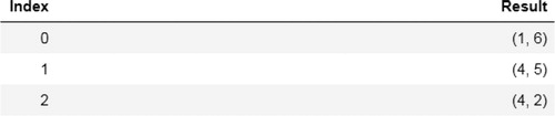
The above code tells Symbulate to draw 2 tickets, with replacement, from a box with tickets labeled 1, 2, 3, and 4. Each simulated outcome consists of an ordered pair of rolls. The.sim() command simulates realizations of probability space outcomes, events, random variables, or random processes. (In Python, the “dot (.)” syntax is akin to “and then,” with the result of the previous operation being passed over the dot into the next operator.) For example, the code below simulates three rolls of two four-sided dice (Figure 1).

Fig. 1 Output of P.sim(3), simulated outcomes of two four-sided dice rolls. (Note that Python uses zero-based indexing.)

P.sim(3)

Next, a random variable is a function that maps outcomes of a probability space to real numbers: $X(\omega )$ for $\omega \in \Omega$, the sample space. A Symbulate RV is specified by the probability space on which it is defined and the mapping function. Thus, the definition of a random variable in Symbulate is consistent with the mathematical definition and reinforces that a random variable is a function.

X = RV(P, sum) Y = RV(P, max)

The above code simply defines the random variables. One key pedagogical feature of Symbulate is the ability to define and manipulate probability spaces and random variables as abstract objects, independently of simulated realizations. Furthermore, the explicit separation in Symbulate between probability space and random variable facilitates understanding of these distinct concepts.

Since a random variable X is a function, any RV can be called as a function to return its value $X(\omega )$ for a particular outcome ω in the probability space.

outcome = (3, 2) # a pair of rolls X(outcome), Y(outcome) Out[]: (5, 3)

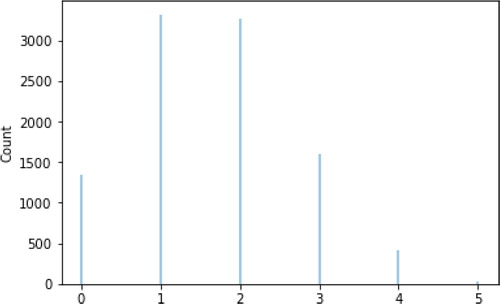
The following commands simulate 10,000 values of the random variable Y, store the results in a variable y, and summarize the realized values and their relative frequencies, in a table and in a plot (Figure 2). (The option normalize = False would return frequencies (counts) rather than proportions.) The code reflects standard notation and emphasizes the explicit distinction between the random variable Y (capital letter) and realized values of it y (small letter).

Fig. 2 Approximate distribution of Y, the maximum of two four-sided dice rolls (table and plot).

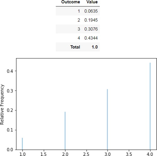
y = Y.sim(10000) y.tabulate(normalize = True) y.plot()

Many descriptive summaries are available, such as the following:

y.count_leq(3)/10000, y.mean(), y.sd() Out[]: (0.5665, 3.1214, 0.9243711592212297)

The values of multiple random variables can be simulated simultaneously, that is, for the same simulated outcomes in the probability space. The following code produces a plot that illustrates the approximate joint and marginal distributions of X and Y obtained by simulation (Figure 3).

Fig. 3 Approximate joint and marginal distributions of X and Y, the sum and maximum of two four-sided dice rolls.

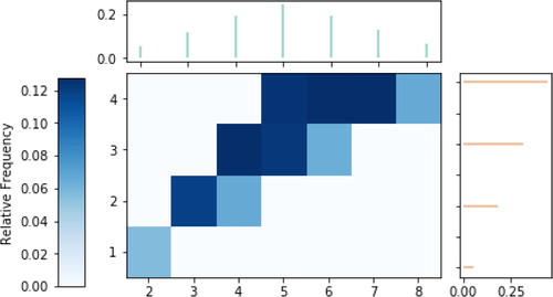
(X & Y).sim(10000).plot( type = ["tile", "marginal"])

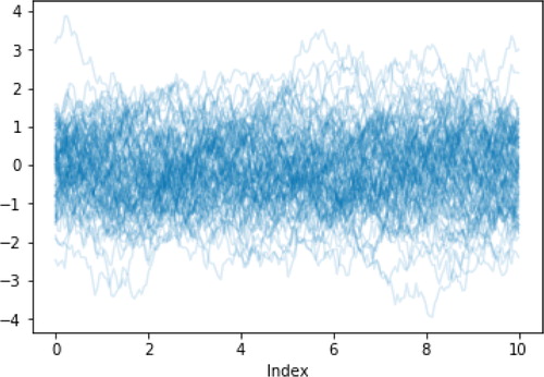
2.2 Stochastic Processes

A stochastic process is an indexed collection of random variables defined on a probability space; the index usually represents time. A realization of a stochastic process X is a sample path of process values over time. A Symbulate random process can be defined via RV on an appropriate probability space. Probability spaces supporting commonly used processes like Poisson processes, Brownian motion, and Gaussian processes are included in Symbulate.

For example, the following code defines a probability space supporting a Poisson process with rate 1, defines the Poisson process N as a (collection of) RVs on this space, and then simulates and plots 100 sample paths of $N$, along with the estimated mean function (Figure 4).

Fig. 4 Sample paths of a Poisson process with rate parameter 1.

P = PoissonProcessProbabilitySpace(rate = 1) N = RV(P) n = N.sim(100) n.plot() n.mean().plot()

The value of a stochastic process X at a particular point in time t is a random variable, typically denoted X_t or X(t). The corresponding syntax for a Symbulate random process X is X[t], which returns an RV object, thus closely mirroring the language of probability. For example, N[1.5] is an $\mathit{RV}$ object representing the value of the process N at time 1.5.

In addition to the process values themselves, other random variables can be defined on the same probability space as a random process. For example, the following defines a random vector of the arrival times on the probability space for the Poisson process.

T = RV(P, arrival_times)

A realization of T is a random sequence of arrival times. Random vectors can be indexed with brackets [], with the RV T[0] representing the time of the first (zeroth in Python) arrival, T[1] the time of the second, and so on.

For N and T defined as above, the following code produces Figure 5 which visualizes the approximate joint and marginal distributions of N[1.5], the process value at time 1.5, and T[2], the time of the third arrival.

Fig. 5 Approximate joint and marginal distributions of $N(1.5)$, the process value at time 1.5, and T₂, the time of the third arrival, for a rate 1 Poisson process N.

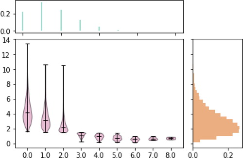
(N[1.5] & T[2]).sim(10000).plot( ["violin", "marginal"])

Custom discrete and continuous time stochastic processes can be constructed with the RandomProcess command. For example, if $Z_0,Z_1,\dots$ are iid with $P(Z_i=1)=P(Z_i=-1)=0.5$ then a simple symmetric random walk $\left\{S_n\right\}$ on the integers satisfies $S_0=0$ and $$S_{n+1}=S_n+Z_n,\hspace{1em}n=1,2,\dots$$

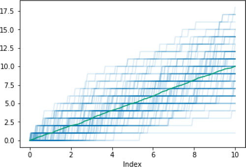
The following code defines such a random walk in Symbulate; index_set = Naturals() represents the discrete time index set $\{0,1,2,\dots \}$. The code reflects that a suitable probability space consists of “equally likely” infinite sequences in ${\{-1,1\}}^{\infty }$, and that a random walk is a sum of iid random variables (and not just simulated values). [There must be an upper bound on the number of steps for computational reasons, hence n in range(100). However, Symbulate does allow sample space outcomes to be represented as infinite sequences.]

P = BoxModel([-1, 1], size = inf, replace = True) X = RandomProcess(P, index_set = Naturals()) Z = RV(P) X[0] = 0 for n in range(100): X[n + 1] = X[n] + Z[n]

The random process X defined in this way can be manipulated like N in the Poisson process example. For example, X.sim(10).plot() produces Figure 6.

Fig. 6 Ten sample paths of a simple symmetric random walk on the integers.

2.3 Commonly Used Probability Models

Many common univariate and multivariate distributions and random processes are available in Symbulate. See Appendix A for a partial list.

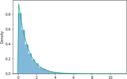
By definition, a random variable must always be a function defined on a probability space. However, in many situations the distribution of a random variable is assumed or specified directly, without mention of the underlying probability space or the function defining the random variable, as in “let X have a N(0, 1) distribution.” The RV command can also be used to define a random variable by specifying its distribution, as in the following code which produces Figure 7.

Fig. 7 Kernel density plot of simulated values of $X\sim N(0,1)$.

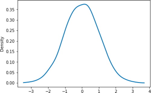
X = RV(Normal(0, 1)) X.sim(10000).plot("density")

Specifying a random variable by specifying its distribution, as in the first line above, has the effect of defining the probability space to be the distribution of the random variable and the function defined on this space to be the identity (f(x) = x). However, it is more appropriate to think of such a specification as defining a random variable with the given distribution on an unspecified probability space through an unspecified function. Such an interpretation emphasizes the difference between a random variable and its distribution.

Many commonly used stochastic processes can be defined as Symbulate random processes directly without first explicitly defining a probability space. For instance, the Poisson process in Section 2.2 can also be defined, without calling PoissonProcessProbabilitySpace, via

N = PoissonProcess(rate = 1)

2.4 Independence

In Symbulate, independence is represented by the asterisk *, which reflects that under independence, “joint” objects (e.g., probability, cdf, pdf) are products of the corresponding “marginal” objects.

In the code below, the probability space P corresponds to a single roll of a fair four-sided die, Q to a single roll of a fair six-sided die, and the product space P * Q to the pair of independent rolls (Figure 8).

Fig. 8 Simulated outcomes of independent dice rolls.

P = BoxModel([1, 2, 3, 4]) Q = BoxModel([1, 2, 3, 4, 5, 6]) (P * Q).sim(3)

When dealing with multiple random variables it is common to specify the marginal distribution of each and assume independence. For example, the following code defines independent random variables X and Y with $X\sim \text{Poisson}\left(1\right)$ and $Y\sim \text{Poisson}\left(2\right)$. The syntax emphasizes that for independent random variables, the joint distribution is the product of the marginal distributions.

X, Y = RV(Poisson(1) * Poisson(2))

The above product syntax also emphasizes that the random variables are defined on the same probability space, the product space defined by Poisson(1) * Poisson(2). An outcome in this product probability space is a pair of values, and X corresponds to the first coordinate of the pair and Y the second.

Because Symbulate mirrors the language of probability so closely, it can actually catch student misconceptions about probability. Continuing the above example, a student who wants to simulate values of X + Y might write the following code, which would produce an error.

X = RV(Poisson(1)) Y = RV(Poisson(2)) (X + Y).sim(10000) # Returns an error: Random variables must be # defined on the same # probability space.

The above code reveals a fundamental flaw in the student’s understanding. The first two lines define the marginal distributions of X and Y. However, the marginal distributions alone are insufficient to specify the joint distribution, and the joint distribution is needed to simulate values of X + Y. The critical missing piece is the assumption of independence. In Symbulate independence must be explicitly specified by the user; it is not assumed by default. The code could be fixed using the “*” syntax as above, or the AssumeIndependent command as follows.

X = RV(Poisson(1)) Y = RV(Poisson(2)) X, Y = AssumeIndependent(X, Y) (X + Y).sim(10000)

The first three lines above are equivalent to X, Y = RV(Poisson(1) * Poisson(2)). Requiring the user to explicitly specify independence—either with * or Assume Independent—emphasizes that independence is an assumption, and also that marginal distributions alone do not fully specify a joint distribution.

The error produced by the code without the Assume Independent line illustrates how Symbulate reflects probability at an even deeper level. Recall that a random variable is function defined on a probability space—$X(\omega )$ for $\omega \in \Omega$—so a sum, for example, of random variables $Z=X+Y$ is a sum of functions, $Z(\omega )=X(\omega )+Y(\omega )$ for $\omega \in \Omega$. Therefore, it does not make sense to add or otherwise transform multiple random variables unless they are defined on the same probability space. Symbulate reflects this concept; attempting to transform random variables defined on different probability spaces will produce an error.

Independence is often assumed. However, independence is determined by the underlying probability measure, and so it does not make sense to even consider independence of random variables unless they are defined on the same probability space. The AssumeIndependent command essentially formalizes the following existence theorem (e.g., Durrett 2010, sec. 2.1.4) encountered in graduate probability courses: there exists a probability space upon which random variables X, Y are defined such that X and Y are independent and have the specified marginal distributions. The AssumeIndependent command constructs, in the background, a probability space from the product of the marginal distributions and defines the random variables via each coordinate. Thus, the functionality of the AssumeIndependent command mirrors the existence theorem and its proof. This is just one example of how Symbulate is consistent with the mathematics of probability, even for advanced concepts covered in graduate courses.

Symbulate will also produce an error when the user tries to force dependent random variables to be independent. Random variables that are defined as explicit functions on a common probability space, such as X and Y in Section 2.1, are either independent or not; there is nothing to assume. Attempting to call AssumeIndependent(X, Y) in such a situation will return an error.

2.5 Events and Conditioning

An event A is a subset of the sample space. When an outcome ω is drawn from the sample space, an event either occurs ($\omega \in A$) or not ($\omega \in A^c$). Likewise, simulating an event A in Symbulate returns True for outcomes when the event occurs and False otherwise. For syntactical reasons, events in Symbulate must be enclosed in parentheses () rather than braces.

For example, let $Z=X+Y$ where X and Y are independent with $X\sim \text{Poisson}\left(1\right)$ and $Y\sim \text{Poisson}\left(2\right)$. The following code defines and simulates the event $A=\{Z>4\}$; see Figure 9.

Fig. 9 Simulated realizations of the event $\{Z>4\}$, where $Z=X+Y$, X and Y are independent, $X\sim \text{Poisson}\left(1\right)$, and $Y\sim \text{Poisson}\left(2\right)$.

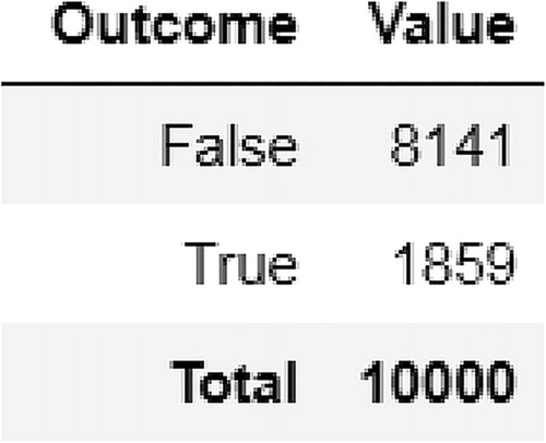
X, Y = RV(Poisson(1) * Poisson(2)) Z = X + Y A = (Z > 4) A.sim(10000).tabulate()

Consistent with standard notation, conditioning on an event in Symbulate is accomplished with the vertical bar — (read “given”). Continuing from the previous example, the following code simulates from the conditional distribution of X given $\{Z=5\}$ and produces the plot in Figure 10. [The double equal sign == represents logical equality.]

Fig. 10 Approximate conditional distribution of X given $\{Z=5\}$.

(X | (Z == 5)).sim(10000) .plot(normalize = False)

Note that.sim(10000) above produces 10,000 realizations from the conditional distribution of X given $\{Z=5\}$. When.sim() is called with conditioning, the simulation runs, rejecting those values for which the conditioning event returns False, until the desired number of repetitions which satisfy the condition is achieved.

See Example 2 in Section 4.2 for further discussion of conditioning.

2.6 Transformations

A transformation of a random variable is also a random variable. If X is an RV and g is a function, X.apply(g) defines a new RV which behaves like any RV. Note that for arithmetic operations and many common math functions (such as exp, log, sin) one can simply call g(X).

For example, the code below produces the plot in Figure 11 which illustrates that if U has a Uniform(0, 1) distribution, then $X=-\hspace{0.17em}\text{log}\hspace{0.17em}(1-U)$ has an Exponential(1) distribution.

Fig. 11 Log transform of a random variable with a Uniform(0,1) distribution.

U = RV(Uniform(0, 1)) X = -log(1 - U) X.sim(10000).plot() Exponential(1).plot() # displays the theoretical pdf

The line X = -log(1 - U) above could be replaced by the following code which uses apply.

def g(u): return -log(1 - u) X = U.apply(g)

As discussed in Section 2.4, transformations of multiple random variables defined on the same probability space are also random variables. In particular, arithmetic operations like addition, subtraction, multiplication, and division can be applied to random variables defined on the same probability space.

2.7 Summary: Pedagogical Implications of Symbulate Syntax

The following list contains just a few examples of how Symbulate syntax reflects the language of probability and reinforces probabilistic concepts, through both what it can and cannot do.

• Probability spaces, events, random variables, and stochastic processes are defined separately from each other, and separately from their simulated values.

• Calling.sim() on a Symbulate object produces an appropriate realization of the object: an outcome for a probability space, True or False for an event, a numerical value for a random variable, and a sample path for a stochastic process. That is, the Symbulate objects behave just like their mathematical counterparts.

• A Symbulate random variable is a function defined on a probability space.

• If X is a random process, X[t] is a random variable representing the process value at time t.

• The product syntax represents independence. It is possible to create a product probability space by multiplying probability spaces, and to specify the joint distribution of independent random variables as the product of their marginal distributions.

• Independence is an assumption. In Symbulate, independence must be explicitly specified by the user; it is not assumed by default. Symbulate prevents users from simulating multiple random variables if only their marginal distributions are provided.

• Conditioning on events is represented by —, and it is possible to simulate directly from a conditional distribution.

• All random variables and random processes in Symbulate must be defined on a probability space, which encourages students to consider what might be an appropriate probability space for a given situation.

The following example, in which we compare Symbulate and R commands, highlights some of the pedagogical advantages of Symbulate, even in situations that might seem relatively straightforward in R.

Consider producing the plot in Figure 10 of the approximate conditional distribution of X given $\{Z=5\}$, with X and Y independent, $Z=X+Y,X\sim \text{Poisson}\left(1\right)$, and $Y\sim \text{Poisson}\left(2\right)$. While there are many ways to program this scenario in R, we think the code on the left requires the least familiarity with R. The comparable Symbulate code is provided on the right (Table 1).

Table 1 Comparison of Symbulate and R commands for the example illustrated in Figure 10.

x = rpois(n = 10000, lambda = 1)	X = RV(Poisson(1))
y = rpois(n = 10000, lambda = 2)	Y = RV(Poisson(2))
	X, Y = AssumeIndependent(X, Y)
z = x + y	Z = X + Y
plot(table(x[(z == 5)])	(X — (Z == 5)).sim(10000).plot()

Comparison of the Symbulate and R commands illustrates how Symbulate more closely reflects the language of probability.

• No random variables are defined in R; x (and similarly y) is merely a vector of values drawn at random from a Poisson distribution. In Symbulate, one can define random variables with the appropriate marginal distributions, which fosters understanding of the distinction between a random variable (X) and realized values of it (x).

• The rpois function takes two arguments, but only one of them is actually a parameter of the distribution. Also, names of R functions for probability distributions are abbreviated and change based on their purpose (e.g., rpois, ppois, dpois). In Symbulate, a distribution is defined by its full name and relevant parameters (see Appendix A).

• In R, x and y can be treated as independent because the values are generated separately. Symbulate explicitly incorporates the assumption stated in the problem that X and Y are independent random variables.

• In R, z is an element-by-element sum of two vectors; in Symbulate, just like in the problem statement, Z is a sum of two random variables.

• In Symbulate, the conditioning notation (X — (Z == 5)) mirrors standard probability notation, and reflects that we are conditioning a random variable on an event. The conditioning is accomplished in R with logical subsetting, x[(z == 5)], an operation which is not entirely straightforward, especially for students with no previous programming experience. In addition, in Symbulate (X — (Z == 5)).sim(10000) simulates 10,000 values directly from the conditional distribution. Simulating exactly 10,000 values from the conditional distribution in R would require additional nontrivial programming.

In addition to the pedagogical advantages of Symbulate syntax, we discuss in Sections 3 and 4 how programming simulations and producing graphics in Symbulate is often considerably easier than in other software packages, especially for students with little experience with programming.

3 Symbulate Graphics

Symbulate enables easy and effective visualization of probability distributions and simulation output. The universal.plot() function infers the “right” type of plot for the given data. For example,.plot() produces, by default,

• an “impulse plot” for a discrete random variable (e.g., Figure 2),

• a histogram for a continuous random variable (e.g., Figure 11),

• a scatterplot for two continuous random variables (e.g., Figure 14),

• a sample path plot for a stochastic process (e.g., Figures 4, 6, 15).

While the default plot is typically an effective visualization of the simulation results, there are several additional options available, including the ability to add marginal distributions (e.g., Figures 3, 5, 13) or plot kernel density estimates (e.g., Figures 7, 13). The Symbulate documentation contains many more examples of Symbulate graphics. [The Python package Matplotlib can be used to further customize plots with titles, legends, labels, etc.]

Furthermore, making multiple calls to.plot() within a Jupyter notebook cell produces a single figure with the graphics superimposed (e.g., Figures 11, 12, 14), enabling easy comparison of distributions without requiring code to organize data in a certain way or adjust axes to combine multiple plots. For example, the following code produces the two superimposed histograms in Figure 12 (note the use of Matplotlib to add a legend and an x-axis label).

Fig. 12 Superimposed histograms.

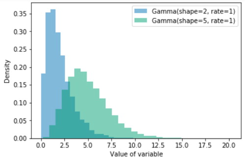
RV(Gamma(shape = 2,rate = 1)).sim(10000).plot() RV(Gamma(shape = 5,rate = 1)).sim(10000).plot() from matplotlib import pyplot as plt plt.legend(["Gamma(shape = 2, rate = 1)", "Gamma(shape = 5, rate = 1)"]) plt.xlabel("Value of variable");

The simplicity of the.plot() function saves students from spending time on trying to get plots to look right. This is especially useful for pure probability courses, where students might not have been exposed yet to exploratory data analysis and visualization, let alone to R or packages like ggplot2. Therefore, Symbulate enables students to focus on how to interpret—rather than how to produce—visualizations of simulation results to understand the relevant distributions.

Symbulate provides a technology tool to “help students visualize concepts and develop an understanding of abstract ideas by simulations” (GAISE College Report ASA Revision Committee 2016, p. 20). For example, the following code produces a visual (Figure 13) which facilitates understanding of joint and marginal densities.

Fig. 13 Bivariate normal distribution: joint and marginal densities.

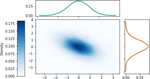
Fig. 14 Joint and joint conditional distributions for Example 2.

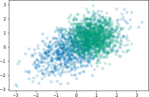
Fig. 15 Sample paths of an Ornstein–Uhlenbeck process.

RV(BivariateNormal(corr=-0.5)).sim(10000).plot( ["density", "marginal"])

In particular, Symbulate enables students to easily witness connections between various different distributions, or to observe how distributions respond to changes in parameter values.

4 Programming With Symbulate

As illustrated by the examples in Section 2, many scenarios require only a few lines of Symbulate code to set up, run, analyze, and visualize. Table 2 comprises the requisite Symbulate commands for a wide variety of situations.

Table 2 Symbulate commands.

Command	Function
ProbabilitySpace	Define a probability space (e.g., BoxModel)
RV	Define random variables, random vectors, or random processes
apply	Apply transformations
[] (brackets)	Access a component of a random vector or a
	random process at a particular time;
	create logical subset in simulation space
* (and **)	Define independent probability spaces or distributions
AssumeIndependent	Assume random variables or processes are independent
| (vertical bar)	Condition on events
&	Join random variables into a random vector;
	simulate multiple random variables (e.g., (X & Y).sim(10000))
sim	Simulate outcomes, events, random variables, and random processes
tabulate	Tabulate simulated values
plot	Plot simulated values
filter (and relatives)	Create subsets of simulated values
Statistical summaries	count (and relatives), mean, median, sd, var, quantile, corr, cov, etc.
Common models	See Appendix A

4.1 Simulation With Minimal Programming

Conducting and analyzing simulations in Symbulate requires minimal programming. Symbulate eliminates the need for: writing loops to perform repetitions of a simulation, initializing and updating variables to store results, “vectorizing” code, and learning commands or packages to produce graphics. In addition, there is no need to install additional packages or libraries.

Therefore, rather than fussing with the syntactical mechanics of coding a simulation or producing a plot, students can focus instead on the core probabilistic elements of the scenario: What are the outcomes in the probability space? What is being measured for these outcomes? What assumptions are being made? What, if anything, is being conditioned on? How do we interpret—rather than produce—visualizations of simulation results to understand the relevant distributions?

In general, Symbulate programs are short, easy to write, run quickly, and produce effective visualizations. The pedagogical impact is an environment where students can readily employ simulation to analyze virtually every probability problem. In fact, one goal of the Symbulate project is to make simulation as ubiquitous as calculus as a tool for analyzing probability problems and understanding probabilistic concepts.

The brevity of most Symbulate programs also makes them relatively easy to debug. In addition, many common mistakes have been anticipated and addressed in docstrings, online documentation, the “Getting Started” tutorial, and error messages.

Of course, one can still have assignments where students write their own code (R, Python) from scratch. Unfortunately, in our experience, when students encounter problems it is often difficult to discern between misunderstanding of probability concepts and trouble with coding and debugging. We agree that it is beneficial for students to consider the process of a simulation (first step, second step, repeat, etc.). However, we prefer to assess understanding of the simulation process with “how would you simulate this with boxes/coins/dice/spinners?” type questions or by asking students to write pseudo-code. Even if it is desired for students to write detailed simulation code for select problems, Symbulate greatly eases the programming burden for all the other ones.

4.2 Comparison With R and Other Simulation Software

R is commonly used to conduct simulations in probability and statistics courses. The example in Section 2.7 highlights some of the pedagogical advantages of Symbulate over R even when the R code is relatively simple. In addition, in many scenarios, such as the following examples, the Symbulate code is significantly easier to write than R code, especially for students who have little experience with programming or R.

Example 1.

Conditioning, with |, is especially easy in Symbulate; it is possible to simulate directly from a conditional distribution without subsetting, if statements, or loops. For example, let (X, Y, Z) have a multivariate normal distribution with mean vector and covariance matrix given in the code below. Suppose we want to produce a single figure with two scatterplots overlaid to illustrate how the joint distribution of Y and Z changes when conditioning on the value of X. (In this case, Y and Z are not independent, but they are conditionally independent given $\{X=x\}$.) The following Symbulate code performs the simulation and produces Figure 14. Note that rather than conditioning on the probability zero event $\{X=1\}$ we condition on $\left\{\right|X-1|<0.01\}$, an event which has probability 0.005. This requires about 200,000 repetitions of the simulation, which run in the background, to produce 1000 values for which the conditioning event is true. [The alpha argument just controls the transparency of the points.]

mu = [0, 0, 0] Sigma = [[1.00, 0.80, 0.70], [0.80, 1.00, 0.56], [0.70, 0.56, 1.00]] X, Y, Z = RV(MultivariateNormal(mean = mu, cov = Sigma)) (Y & Z).sim(1000).plot(alpha = 0.2) ((Y & Z) | (abs(X - 1) < 0.01)).sim(1000) .plot(alpha = 0.2)

The comparable base R code below involves installing the MASS package to use the mvrnorm function, logical subsetting and indexing of matrices, and some plotting issues, including using two different functions, plot and points.

mu = c(0, 0, 0) Sigma = rbind(c(1.00, 0.80, 0.70), c(0.80, 1.00, 0.56), c(0.70, 0.56, 1.00)) library(MASS) xyz = mvrnorm(n = 1000, mu = mu, Sigma = Sigma) xyz_given_x1 = mvrnorm(n = 200000, mu = mu, Sigma = Sigma) xyz_given_x1 = xyz_given_x1 [abs(xyz_given_x1[, 1] - 1) < 0.01,] plot(xyz[, 2], xyz[, 3], col="skyblue") points(xyz_given_x1[, 2], xyz_given_x1[, 3], col="seagreen")

In R, simulating roughly 1000 pairs for which the conditioning event is true requires the user to figure out in advance how many pairs to simulate in total (200,000 above). Furthermore, the conditioning is accomplished with logical subsetting, an operation which is not entirely straightforward, especially for students with no previous programming experience. Simulating exactly 1000 pairs from the conditional distribution in R would require additional nontrivial programming (e.g., a while loop which stops when the target of 1000 is achieved). In contrast, in Symbulate calling.sim(1000) in the presence of conditioning simulates 1000 values directly from the conditional distribution.

Example 2. A

s illustrated in Section 2.2, working with stochastic processes in general, and continuous time processes in particular, is relatively straightforward in Symbulate. As another example, the following code simulates and displays (Figure 15) 100 sample paths of an Ornstein–Uhlenbeck process, defined as a Gaussian process with a particular mean function and autocovariance function.

def mean_fn(t): return 0 def cov_fn(s, t): return exp(-abs(s-t)/2) U = GaussianProcess(mean_fn, cov_fn) U.sim(100).plot()

The process U can also be defined as a time-rescaled Brownian Motion as in the code below. ContinuousTime Function() represents the deterministic process f(t) = t.

B = BrownianMotion(drift = 0, scale = 1) t = ContinuousTimeFunction() U = exp(-t/2) * B(exp(t))

While there are R packages for stochastic processes, we know of no way to program this example that is as simple as the Symbulate code above, which simply: (1) defines the process, (2) simulates 100 paths of it, and (3) plots the paths.

With a language like R, the user has many options when coding a scenario (e.g., loops vs. vectorizing). Unfortunately, such flexibility can be a detriment to students, especially those with little programming experience, who often get lost among all the possibilities. Students in a probability course that incorporates simulation essentially have to learn two languages: the language of probability and the language of the simulation software package. The Symbulate package attempts to streamline this learning process, by making the language of the simulation software resemble as closely as possible the language of probability. Thus, a user’s choice for how to program a scenario in Symbulate is determined by its core probabilistic elements, rather than by peripheral programming considerations.

In addition to R, several software packages have simulation capability, including NumPy/SciPy (for Python), Matlab, and Mathematica. Many of our comments about R also apply to these software packages; however, we do not provide detailed comparisons here. Table 3 provides some evidence that, in particular, Symbulate syntax for working with common distributions is simpler and more intuitive than that of other popular software packages, which use commands that contain abbreviations, mix parameters of the distribution with arguments of the command, or change syntax depending on the context.

Table 3 Comparison across packages of syntax for a Normal(0, 1) distribution.

	Simulate 1000 values	Evaluate the CDF at 2
Symbulate	Normal(0, 1).sim(1000)	Normal(0, 1).cdf(2)
R	rnorm(1000, 0, 1)	pnorm(2, 0, 1)
NumPy	random.normal(0, 1, 1000)	(not possible)
SciPy	norm(0, 1).rvs(1000)	norm(0, 1).cdf(2)
Matlab	normrnd(0, 1, 1000, 1)	normcdf(2, 0, 1)
Mathematica	RandomVariate[	CDF[NormalDistribution[0, 1], 2]
	NormalDistribution[0, 1], 1000]

Symbulate does employ the NumPy and SciPy libraries in the background. For example, the Symbulate command Normal(0, 1).sim(1000) is essentially a wrapper for the NumPy command random.normal(0, 1, 1000). For common probability models, the Symbulate source code uses the tools available in NumPy and SciPy; Symbulate just codifies the syntax. However, Symbulate’s design also incorporates many innovative features for running simulations. Technological innovations from the software development perspective will be discussed in a forthcoming paper (Sun and Ross (2019).)

Symbulate and the aforementioned software packages require some programming. On the other hand, many online applets (Siegrist 2017; Dinov et al. 2016; Kahle 2014; Rossman and Chance 2017) can simulate various probability models via point-and-click interfaces which require no programming from the user. While applets have many appealing features, Symbulate still has many advantages.

• Applets are only available for certain problems or situations. For example, we know of no applets for Examples 1 and 2 in this section, or for many of the previous examples. Furthermore, designing an applet for a new situation (e.g., using Shiny (Doi et al. 2016)) can require significant programming and testing.

• Existing applets are not-customizable; users are limited to the choices available, especially with respect to graphics. For example, an applet might only display a scatterplot, while Symbulate allows the user to also produce a two-dimensional histogram or density plot.

• The large majority of available applets focus on univariate distributions. In contrast, Symbulate has wide capability for multivariate distributions and stochastic processes.

• Interfaces vary from applet to applet, and so each applet comes with some start-up cost. Symbulate provides a consistent syntax across all scenarios.

• Applets do not provide any of the pedagogical benefits that come with actually coding a simulation. When writing Symbulate code, students must program the core elements of the scenario and speak the language of probability, thus practicing and reinforcing their understanding of probabilistic concepts.

4.3 Simulation Space Operations

A key technological feature of Symbulate is the availability of random variable space operations: the ability to define and manipulate random variables (and probability spaces, events, and stochastic processes) as abstract objects, independently of simulated realizations. The examples thus far illustrate various random variable space operations. Many of the key pedagogical benefits of Symbulate stem from the existence of random variable space.

Random variable space operations also have simulation space counterparts. That is, realizations from a simulation can be stored and manipulated directly without having to redefine random variable space objects. For example, for a RV X, Y = exp(X) is a random variable space operation, while x = X.sim(100); exp(x) represents a simulation space operation. Simulation space operations are vectorized and provide an “R like” way to interact with Symbulate.

Consider the example in Section 2.7. The following Symbulate code produces a plot similar to Figure 10; the last three lines contain simulation space operations.

X = RV(Poisson(1)) Y = RV(Poisson(2)) X, Y = AssumeIndependent(X, Y) xy = (X & Y).sim(10000) x = xy[0] z = xy[0] + xy[1] x[z == 5].plot()

The simulated (X, Y) pairs are stored in the matrix xy with two column vectors, xy[0] and xy[1]. These vectors can be added in a parallel manner to obtain z. Notice that it is not necessary to first define Z = X + Y in random variable space. Logical subsetting (a.k.a. boolean masking) is also possible in simulation space, as in x[z == 5]. However, note that subsetting in simulation space only returns a subset of the simulated values (about 1000 in this case) that satisfy the condition, in contrast to conditioning in random variable space, as in Section 2.7, which produces the specified number of simulated values directly from the conditional distribution.

An important caveat is that simulation space operations are only allowed for results from the same simulation. This restriction prevents mistakes that arise when attempting to manipulate results simulated from marginal distributions rather than from a joint distribution. For example, the following code would return an error since the x and y values result from different simulations.

X, Y = RV(BivariateNormal(corr = 0.7)) x = X.sim(10000) y = Y.sim(10000) x + y # Returns error: Results objects must come from the same simulation.

Along the lines of the discussion in Section 2.4, the above error prohibits the user from incorrectly using the vector x + y to approximate the distribution of the random variable X + Y.

While simulation space capability is sometimes useful, we do encourage users to work with random variable space operations whenever possible to realize Symbulate’s benefits most fully.

4.4 Symbulate and Python Programming

While Symbulate uses Python as a platform, most of the features of the Symbulate package itself require no knowledge of Python (and little or no experience with programming in general). It is certainly possible for instructors and students to use Symbulate in a wide variety of contexts without ever using any non-Symbulate commands or writing any general Python code. If Python code is needed, instructors could provide students with the commands (e.g., list(range(1, n + 1)) to produce $[1,\dots ,n]$).

However, Symbulate can be used as a framework for introducing students to Python—one of the most widely used programming languages in the world—and experience with Python is becoming increasingly important for students interested in data science. In particular, students can use Python to write functions or loops to define or transform random variables or stochastic processes, or to investigate the effects of changing parameter values (as in the example in Section 5.2).

The basic elements of a Symbulate program are the same as the basic elements of a probability model: probability space, events, random variables, stochastic processes. Symbulate has many common probability spaces and processes built in, but it is still possible, and sometimes necessary, to incorporate programming to define custom probability spaces and functions. The following example illustrates how Symbulate and Python commands can be combined to handle problems that do not involve familiar distributions.

Example 1.

The “coupon collector’s problem” is a classic problem of probability (Mosteller 1987). Consider a brand of cereal that, as a promotion, includes a prize (or coupon) inside every cereal box. The prize in each box is equally likely to be any one of n distinct types. Typical versions of the problem involve the number (X) of boxes needed to obtain a complete set of the n types. But suppose we are interested in the relationship between X and other random variables, such as the maximum number (Y) of prizes collected of any type. For example, the following code provides a simulation-based estimate of $E(X|Y\le 3)$, the conditional expected value of the number of boxes needed to complete a set of n = 6 given that at most three prizes of any type are collected.

n = 6 prizes = list(range(n)) P = BoxModel(prizes, size = inf) def number_prizes_and_max_count(outcome): prizes_so_far = [] for i, prize in enumerate(outcome): prizes_so_far.append(prize) if len(set(prizes_so_far)) == n: return i + 1, max(prizes_so_far.count(j) for j in prizes) X, Y = RV(P, number_prizes_and_max_count) (X | (Y < = 3)).sim(10000).mean()

Even though the above involves Python code, incorporating Symbulate commands simplifies the programming and emphasizes the core probabilistic elements.

• The probability space, in which an outcome ω corresponds to a sequence of prizes selected, is defined as its own object. Any number of random variables can be defined on the probability space.

• Symbulate allows outcomes of a probability space to be infinite sequences. Such a representation is convenient in the coupon collector problem, for example, when considering the number of prizes selected until r sets are completed. (Probability spaces in which outcomes are infinite sequences are common when working with stochastic processes.)

• Non-Symbulate commands are primarily used to define the function number_prizes_and_max_count. This function codes the mapping of an outcome ω to the output $X(\omega )$, $Y(\omega )$. Programming a function for use in defining a Symbulate RV reinforces the concept that a random variable is, by definition, a function. (We find that writing functions to define random variables, vectors, or processes is where much of the non-Symbulate programming occurs in “advanced” examples. To minimize programming, custom functions could be provided to students to use along with built-in functions like sum or log.)

• The basic mechanics of running the simulation are handled with.sim() without any further programming (e.g., loops). Thus, Symbulate focuses attention on writing commands to define the probability model, rather than those needed to run the simulation.

• Conditioning on (Y ¡= 3) simulates 10,000 values directly from the conditional distribution without the need for additional programming.

The example illustrates that even in situations that involve non-Symbulate programming, incorporating Symbulate commands as much as possible reinforces the language of probability in ways in which programming alone does not.

5 Using Symbulate in the Classroom

5.1 Considerations When Choosing Software

There are obviously many issues to consider when choosing which software (R, Matlab, Python, etc.) to use in a probability course. We now discuss our perspectives on some of these issues and why we think Symbulate is an option well worth considering.

Our primary goal of using software in probability courses is to support student learning of probability concepts. We have discussed throughout this paper the many pedagogical benefits of Symbulate: how it streamlines the software experience to minimize programming and reflect the language of probability, so that students can focus on learning probability rather than on programming or syntax.

Student software use can take a variety forms, from making minor revisions to code provided by the instructor to writing everything from scratch. Providing code to students allows them to easily investigate many problems and examples, but do they learn the software? On the other hand, if students need to code everything from scratch, time and attention is shifted away from learning probability to coding and debugging. One way to compromise is to have students interact with the software primarily via packages (e.g., Symbulate, Mosaic) rather than in the base language (e.g., Python, R). Students who use Symbulate can still be required to write code for almost every problem, but the syntax and programming is targeted around the core probabilistic elements of the scenario.

It could be argued that using R (or Matlab or Python) provides students with valuable job skills. However, the burden of learning a programming language should not fall on a probability course. Students already have enough difficulty learning probability without having to learn a new programming language too. As an analogy, while some instructors use R in introductory statistics courses, many do not; there are pedagogical and practical advantages and disadvantages to each approach. In our opinion, many of the same considerations apply to introductory probability courses. R is certainly not the default option for introductory statistics courses, and we think it need not be the default option for introductory probability courses either.

Furthermore, students from a variety of fields take probability courses; no one package will satisfy the needs of all students. Statistics majors might benefit from more exposure to R, engineering majors to Matlab, computer science majors to Python. (Instructors could allow individual students to choose from among several packages, but that creates additional issues.) However, all students can probably benefit from knowing a little Python and, as discussed in Section 4.4, Symbulate can provide an introduction to Python.

Just as many students do not progress beyond introductory statistics, a first course in probability is the only class in statistics or probability that some students take. If these students were to use R to run and analyze simulations in a single introductory course, how much R would they really learn? Should cursory exposure to R take precedence over other pedagogical considerations?

Even for statistics majors and students with R experience, using Symbulate offers the many pedagogical benefits to learning probability discussed throughout this paper. Symbulate can be used in a first course in probability, as well as advanced courses in stochastic processes or mathematical statistics. Instructors could incorporate both Symbulate and R, perhaps using R in a few detailed programming assignments requiring students to code a simulation from scratch, while using Symbulate to quickly program and investigate all other problems.

Finally, Symbulate simplifies the production of graphics considerably. In other languages, additional programming beyond that needed to run the simulation would be required to produce graphics like those throughout this paper (e.g., Figures 3, 4, 12, 13). While learning how to produce graphics (e.g., with ggplot2) is obviously a valuable skill, it should not come at the expense of learning probability in a probability course.

5.2 Jupyter Notebooks

While not necessary, we strongly encourage users to interface with Symbulate via Jupyter notebooks. Similar to the R Notebook feature in RStudio, a Jupyter notebook is a document with cells containing either markdown text or code that can be executed interactively, with output visible immediately beneath the input. Jupyter notebooks provide a user-friendly interface supporting interactive and reproducible programming and documentation (Baumer et al. 2014).

Interactivity can be further enhanced through the use of Jupyter widgets which create user interface controls (e.g., sliders, dropdown boxes) for interactively exploring how output responds to changes in parameters. Widgets provide a way to “applet-ize” Symbulate programs. For example, the following Symbulate code simulates and displays (as in the plot in Figure 16) the sampling distribution of the standardized sample mean for iid samples of size n from a population distribution.

Fig. 16 Sampling distribution of the standardized sample mean, with a slider for n (n = 5 is displayed).

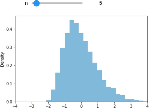
population = Exponential(1) n = 5 RV(population ** n, mean) .sim(10000).standardize().plot()

Adding just a few lines of Python code to incorporate a Jupyter widget creates an interactive central limit theorem demo (Figure 16) with a slider corresponding to the value of n ($n=1,2,\dots ,50$) which updates the plot as the user moves the slider. (It is also possible to add a widget (e.g., dropdown box) corresponding to the population distribution.)

population = Exponential(1) def CLT(n): RV(population ** n, mean) .sim(10000).standardize().plot() plt.xlim(-4, 4) plt.show() from ipywidgets import interact import ipywidgets interact(CLT, n = ipywidgets .IntSlider(min = 1, max = 50, step = 1, value = 1));

Adding a widget does involve some ancillary programming. However, as the above example illustrates, it is relatively straightforward to separate the code essential to the probability model and the simulation from that which relates to the widget. An instructor can provide a scaffold with the widget code and require students to write only the Symbulate commands needed to define the probabilistic elements of the scenario. Even in classes where students do not write Symbulate code themselves, instructors can employ Symbulate and widgets to interactively demonstrate a variety of concepts.

5.3 Symbulate Resources

There are a number of resources for getting help with Symbulate, many of which can be found at the Symbulate Github repository, including:

• Comprehensive documentation of the Symbulate package with numerous examples.

• A collection of Jupyter notebooks containing an interactive “Getting Started with Symbulate” tutorial.

• Command line help within a Jupyter notebook, available by calling? followed by the name of the command (e.g.,? BoxModel) to access the docstring with information on syntax and functionality.

• Helpful error and warning messages which address Symbulate syntax as well as the underlying probabilistic concepts, targeted specifically at the audience of a first course in probability.

Additional materials such as “how to” videos and FAQs are under development. The Github site also provides a natural platform where Symbulate users can interact and share resources.

While the focus of Symbulate is on simulation, Symbulate can also function as an analytical distribution calculator for common distributions. See Appendix A for some examples. Note that the syntax again mirrors the language of probability, for example,.cdf() for cumulative distribution function,.pdf() for probability density function.

5.4 Instructor and Student Experience With Symbulate

To date, we have primarily used Symbulate in two courses, each a calculus-based first course in probability at the level of Carlton and Devore (2017). A typical section had 35 students and met for four 50 min lecture periods per week for 10 weeks.

• Probability and Random Processes for Engineers (Course A): A course for undergraduate Electrical Engineering and Computer Engineering majors which included some coverage of stochastic processes. While the course had no computing prerequisite, most of the students had programming experience, many with Python. One lecture period per week was held in a computer lab classroom where students spent almost all of class time working in pairs on a Symbulate lab like the one in Appendix B.

• Introduction to Probability and Simulation (Course B): A course primarily for undergraduate Statistics, Mathematics, and Computer Science majors, which had a computing prerequisite and an emphasis on simulation. Students primarily used Symbulate outside of class to complete weekly assignments similar to the one in Appendix B.

Initially, students were required to install Symbulate on their personal computers. We recommend the Python installation Anaconda, which can be downloaded and installed in a manner similar to that for R/RStudio. Symbulate can be installed at the command line, similar to using install.packages in R. The level of technical difficulty encountered when installing Symbulate is comparable to what we have experienced with other programs (e.g., R/RStudio).

In more recent offerings, students have interacted with Symbulate through an online server running JupyterHub (similar to RStudioServer), which requires no installation from the user.

Based on our experience, we strongly recommend dedicating some class time to student work on Symbulate. The introduction of the lab hour provided students more opportunities to actively practice speaking the language of probability by writing and discussing Symbulate code and examples with their partners, and helped integrate Symbulate more fully into the class curriculum. During the lab hour we circulated around the room and answered student questions. When students encountered errors in Symbulate code, we could engage them in conversations about probability concepts, like in the independence example in Section 2.4.

In addition to assignments, throughout the course we provided demos of Symbulate during lecture—for almost every topic—and posted examples like those in the previous sections on the course website. While this is of course possible with any software, we found that Symbulate encouraged and enabled us to use simulation-based illustrations more often than we had done previously (using R) and to use more and better graphics. We found that Jupyter widgets (Section 5.2) made it relatively easy to create interactive demos.

Appendix C summarizes the results of informal survey of 93 students enrolled in Course A and 70 students enrolled in Course B. (Students received a small amount of quiz credit for participating.) The survey gauged student opinions of the role that simulation in general, and Symbulate in particular, played in the course. Students generally had positive opinions of Symbulate. The most common complaints involved criticisms of the documentation. We have already revised the package to reflect many of the students’ suggestions, most notably by updating the online documentation, revising error messages and docstrings to be more helpful when addressing common mistakes, and creating an interactive “Getting Started with Symbulate” tutorial.

We realize that the survey results provide only anecdotal evidence in favor of using Symbulate in teaching probability. We plan to conduct more formal comparative assessments in the future, but we are encouraged by our experience with Symbulate so far. We will continue to develop and assess Symbulate to make it an even more effective tool for learning probability.

6 Summary

The recommendations in the Guidelines for Assessment and Instruction in Statistics Education (GAISE) College Report (GAISE College Report ASA Revision Committee 2016) refer specifically to courses in statistics. However, Symbulate facilitates the adoption of similar educational principles in probability courses.

• Students can gain experience with multivariable thinking, by using Symbulate to study joint and conditional distributions or stochastic processes.

• Symbulate eliminates much of the computational burden in programming simulations or producing graphics, allowing students to focus on conceptual understanding of probabilistic concepts.

• Symbulate-based labs and activities foster active learning.

• Symbulate provides a technology to explore conceptual ideas and enhance student learning.

Symbulate commands complement the basic terminology and notation of probability, and should be natural to anyone learning or familiar with probability. Writing Symbulate code allows students to practice the language of probability and reinforces understanding of probabilistic concepts. Symbulate requires minimal programming and is accessible to students with little to no programming experience. Symbulate enables easy and effective visualization of probability distributions, which facilitates understanding of abstract concepts and multivariate relationships.

Symbulate includes a large collection of probability models and can be used with a wide variety of concepts and problems involving probability and simulation. We believe that there are few, if any, concepts or problems introduced in typical undergraduate courses covering probability that Symbulate cannot address. Furthermore, Symbulate is a valuable resource for instructors and students in advanced undergraduate and graduate courses that have a more rigorous treatment of probability, or that cover stochastic processes such as Markov chains and Brownian motion.

While Symbulate currently has broad capability, we continue to develop the package, with plans to add even more models (e.g., renewal processes, diffusion and jump diffusion processes) in the near future. We also continue to improve documentation and resources, to incorporate more examples and activities, helpful error messages, and answers to frequently asked questions.

Acknowledgments

We thank the Frost Research Fellows, Robert Cenon, Jack Conway, Howard Liu, and Kien Nguyen, recipients of a Frost Undergraduate Student Research Award, for their contributions to the Symbulate package. We thank students in our sections of STAT 305 and STAT 350 for their feedback. We thank the two anonymous reviewers and the associate editors for their comments.

Additional information

Funding

We are grateful to the Bill and Linda Frost Fund for funding parts of this research.

Appendix A:

Some Distributions and Processes Available in Symbulate

Continuous univariate distributions

• Uniform

• Beta

• Normal

• Exponential

• Gamma

• ChiSquare

• F

• StudentT

• Cauchy

• LogNormal

• Pareto

• Weibull

• Rayleigh

Multivariate distributions

• BivariateNormal

• MultivariateNormal

• Multinomial

Discrete univariate distributions

• DiscreteUniform

• Binomial

• Poisson

• Geometric

• NegativeBinomial

• Pascal

• Hypergeometric

Stochastic processes

• MarkovChain (discrete time)

• ContinuousTimeMarkovChain

• PoissonProcess

• GaussianProcess

• BrownianMotion

• Geometric Brownian motion

• Brownian bridge

• Ornstein Uhlenbeck process

• Random Walk

• ARMA

As illustrated in the examples below, the following methods can be called for named distributions to compute various theoretical quantities.

• .cdf() for cumulative distribution function

• Exponential(1).cdf(2)

• Out[]: 0.8646647167633873

• .pdf() for probability density function if continuous, probability mass function if discrete

• Normal(0, 1).pdf(0)

• Out[]: 0.3989422804014327

• Binomial(10, 0.3).pdf(2)—

• Out[]: 0.23347444049999999

• .mean() for expected value and.var() for variance

• Cauchy(0, 1).mean()

• Out[]: nan

• Binomial(10, 0.3).var()—

• Out[]: 2.0999999999999996

• .quantile() for the quantile function

• Normal(0, 1).quantile(0.975)

• Out[]: 1.959963984540054

Appendix B:

Sample Symbulate Lab

[Note: This lab was assigned after covering discrete and continuous random variables and independence, but before covering Poisson processes. Students downloaded a Jupyter notebook containing the following text and placeholders for their code. Students uploaded their completed notebooks to the course management system and we reran and graded them.]

In this lab you will use the Symbulate package. You are strongly encouraged to refer to the Symbulate documentation as well as the examples posted on the course website. Aside from part e) you should use Symbulate commands whenever possible. If you find yourself writing long blocks of Python code, you are probably doing something wrong. For example, you should not need to write any for loops.

To use Symbulate, remember to first run (SHIFT-ENTER) the following commands.

from symbulate import *

Setup

Suppose that (harmless) micrometeors strike the International Space Station (ISS) at rate 1.5 per hour on average. You will consider three models of how the strikes occur over time.

• Model 1: Strikes occur independently of each other, in each minute of time there is at most one strike, and the probability that a strike occurs in any minute is 1.5/60.

• Model 2: Over any period of time, the number of strikes which occur has a Poisson distribution, and the numbers of strikes which occur in nonoverlapping time periods are independent.

• Model 3: The time elapsed between any two strikes has an Exponential distribution with mean 40 minutes, and the times between strikes are independent.

Model 1

Suppose that strikes occur independently of each other, in each minute of time there is at most one strike, and the probability that a strike occurs in any minute is 1.5/60. (Why is 1.5/60 a reasonable value for the probability?)

(a) Use simulation to approximate the distribution of the number of strikes that occur in the next 3 hours. Make a plot of the distribution, and approximate the mean and the variance.

|### Type your Symbulate commands here and SHIFT-ENTER to run.|

(b) Approximate the probability that there are at least 8 strikes in the next 3 hours.

Model 2

Now suppose that over any period of time, the number of strikes which occur has a Poisson distribution, and the numbers of strikes which occur in nonoverlapping time periods are independent.

(c) Use simulation to approximate the distribution of the number of strikes that occur in the next 3 hours. Make a plot of the distribution, and approximate the mean and the variance. (Hint: Based on the rate at which meteors strike the ISS, what must the mean of the Poisson distribution be?)

(d) Approximate the probability that there are at least 8 strikes in the next 3 hours.

Model 3

Now suppose that the time elapsed between any two strikes has an Exponential distribution with mean 40 minutes, and the times between strikes are independent. (Why is 40 minutes a reasonable value for the mean?)

(e) Use simulation to approximate the distribution of the number of strikes that occur in the next 3 hours. Make a plot of the distribution, and approximate the mean and the variance. (Hint: The exponential RVs represent the time between strikes, or interarrival times. Simulate infinitely many interarrival times using

P = Exponential(…) ** inf

Then, define a Python function count_strikes_in_ 3_hours(…) that takes each infinite sequence of interarrivals and counts up how many strikes there were in the first 3 hours. Finally, define a random variable on the probability space P using your function.)

(f) Approximate the probability that there are at least 8 strikes in the next 3 hours.

Comparison of models

Review your answers for the three models. In each model, we made what appeared to be different assumptions. Does it seem that the distribution of the number of strikes is the same under each of these sets of assumptions? Discuss briefly.

Type your comments here.

Submission Instructions

Before you submit this notebook, click the “Kernel” drop-down menu at the top of this page and select “Restart and Run All”. This will ensure that all of the code in your notebook executes properly. We will rerun your notebook before grading your answers. You will lose points for a notebook with cells that do not run, even if your answers are correct, so please do not skip this step.

Appendix C:

Summary of Survey Results for Student Symbulate Users

Table

		Strongly				Strongly	No
	Course	Agree	Agree	Neither	Disagree	Disagree	Response
The course provided evidence that simulation provides an effective tool for analyzing probability models.	A	29%	52%	6%	0%	0%	13%
	B	50	26	3	0	0	21
Tactile simulations (dice, Duplos, etc) facilitated my understanding of probability concepts.	A	43	32	11	1	0	13
	B	39	29	10	1	0	21
Visualizing simulation results in graphs facilitated my understanding of probability concepts.	A	33	43	9	1	0	14
	B	36	36	4	0	0	24
Performing and analyzing simulations using Symbulate facilitated my understanding of probability concepts.	A	20	46	12	4	1	16
	B	20	39	16	3	0	23
The syntax of Symbulate complemented the “language of probability”.	A	20	44	17	5	0	13
	B	17	44	13	1	1	23
The syntax of Symbulate facilitated my understanding of the “language of probability”.	A	17	32	29	9	0	13
	B	9	29	27	9	3	24
In general, the use of simulation facilitated my understanding of probability concepts.	A	28	53	4	1	1	13
	B	31	34	7	0	0	27
In general, the use of Symbulate facilitated my understanding of probability concepts.	A	19	52	11	4	1	13
	B	11	43	17	4	3	21
		Symbulate	R	Python	Matlab	Other	Response
If you had to do it over, which one of the following would best represent the software you would prefer to use?	A	66%	2%	6%	8%	2%	16%
	B	39	17	14	0	6	24

References

- Baumer, B., Cetinkaya-Rundel, M., Bray, A., Loi, L., and Horton, N. J. (2014), “R Markdown: Integrating a Reproducible Analysis Tool Into Introductory Statistics,” Technology Innovations in Statistics Education, 8. Available at https://escholarship.org/uc/item/90b2f5xh
- Carlton, M. A., and Devore, J. L. (2017), Probability With Applications in Engineering, Science, and Technology, Springer Texts in Statistics (2nd ed.), Cham: Springer.
- Dinov, I. D., Siegrist, K., Pearl, D. K., Kalinin, A., and Christou, N. (2016), “Probability Distributome: A Web Computational Infrastructure for Exploring the Properties, Interrelations, and Applications of Probability Distributions,” Computational Statistics, 31, 559–577. DOI: 10.1007/s00180-015-0594-6.
- Doi, J., Potter, G., Wong, J., Alcaraz, I., and Chi, P. (2016), “Web Application Teaching Tools for Statistics Using R and Shiny,” Technology Innovations in Statistics Education, 9. Available at https://escholarship.org/uc/uclastat_cts_tise/9/1
- Durrett, R. (2010), Probability: Theory and Examples, Cambridge Series in Statistical and Probabilistic Mathematics (Vol. 31, 4th ed.), Cambridge: Cambridge University Press.
- GAISE College Report ASA Revision Committee (2016), The GAISE (Guidelines for Assessment and Instruction in Statistical Education) College Report, Alexandria, VA: The American Statistical Association.
- Garfield, J., and Ben-Zvi, D. (2007), “How Students Learn Statistics Revisited: A Current Review of Research on Teaching and Learning Statistics,” International Statistical Review, 75, 372–396. DOI: 10.1111/j.1751-5823.2007.00029.x.
- Kahle, D. (2014), “Animating Statistics: A New Kind of Applet for Exploring Probability Distributions,” Journal of Statistics Education, 22, 1–21.
- Mosteller, F. (1987), Fifty Challenging Problems in Probability With Solutions, North Chelmsford, MA: Courier Corporation.
- Rossman, A., and Chance, B. (2017), “Rossman/Chance Applet Collection.” Available at http://www.rossmanchance.com/applets/index.html
- Siegrist, K. (2017), “Random (Formerly Virtual Laboratories in Probability and Statistics).” Available at https://www.randomservices.org/random/apps/index.html
- Sun, D. L., and Ross, K. (2019), “Symbulate: A Python Library for Simulating Probability Models,” Working Paper.