Why We Should Teach Causal Inference: Examples in Linear Regression With Simulated Data

Abstract

Basic knowledge of ideas of causal inference can help students to think beyond data, that is, to think more clearly about the data generating process. Especially for (maybe big) observational data, qualitative assumptions are important for the conclusions drawn and interpretation of the quantitative results. Concepts of causal inference can also help to overcome the mantra “Correlation does not imply Causation.” To motivate and introduce causal inference in introductory statistics or data science courses, we use simulated data and simple linear regression to show the effects of confounding and when one should or should not adjust for covariables.

Keywords:

• Bias
• Confounding
• Data generating process
• Directed acyclic graph
• Model interpretation
• Statistical paradoxes

1 Introduction

For some time now, there has been a call for the integration of causal inference in introductory statistics (or data science) courses (e.g., Cummiskey et al. 2020; Hernán, Hsu, and Healy 2019; Kaplan 2018; Ridgway 2016). The Book of Why (Pearl and Mackenzie 2018) increased the motivation to teach concepts that Pearl calls the causal revolution, see, for example, the interview of JSE’s editor Jeff Witmer (Rossman and Witmer 2019).

The Guidelines for Assessment and Instruction in Statistics Education (GAISE, Wood et al. 2018) recommend “Give students experience with multivariate thinking.” However, multivariate modeling can be misleading through the presence of confounding variables such as the well-known Simpson’s or Berkson’s paradoxes. Given the fact that (observational) data are ubiquitous, we concur that today’s students should learn to think even more thoroughly about the data generating process to draw conclusions from data.

The basic ideas of causal inference, for example, directed acyclic graphs, the difference between observing and manipulating data, and counterfactual evaluation may foster a deeper understanding of what can and—maybe even more important—what cannot be deduced by simple data analysis. There are some (introductory) textbooks that address this topic (e.g., Gelman and Hill 2012; Kaplan 2011) but as more and more courses use a (generalized) linear modeling approach to teach statistical thinking (see, e.g., Lindeløv 2019) we tried to combine these ideas. Since causal inference puts a focus on assumptions in the data generating process, we decided to use simulated data (see, e.g., Jamie 2002) instead of real data (which is normally preferred) as the students can see how the data is generated—and how the conclusions based on the data analysis may be flawed.

When teaching statistics and data science in the 21st century, what do you think is most relevant for a data literate individual (see, e.g., Gould 2017)?

He/she should be able to …

1. calculate the median of grouped numeric data (i.e., histogram data);

2. discuss the scenarios for a t-test with or without equal variances as well as the use case for the Wilcoxon–Mann–Whitney-test;

3. program cool code and fancy graphics;

4. think clearly about association and causation.

Of course, there is nothing wrong with any of these, but to prevent “cargo-cult statistics” (Stark and Saltelli 2018) and to “focus on what can go wrong in the application of statistics” (Steel, Liermann, and Guttorp 2019), we try to help students not only to think with data (Hardin et al. 2015; Pruim, Kaplan, and Horton 2017) but also beyond data by giving more time to the topics of association and causation.

2 Causal Inference

As argued by, for example, Schield (2018), we are living in a world full of multivariate observational data, where confounding can be a serious issue for drawing conclusions. But students want to (and should) learn about this (compare the example “How much is a fireplace worth?” in Rossman and De Veaux (2016), see also Cummiskey et al. (2020)).

There are different philosophical and epistemological aspects and statistical approaches to causality which we will not address here. For good introductions to the potential outcomes framework or the directed acyclic graphs (DAG), we direct the reader to Elwert (2013), Pearl, Glymour, and Jewell (2016), Peters, Janzing, and Schölkopf (2017), Morgan and Winship (2015), Imbens and Rubin (2015), and Angrist and Pischke (2014), among many others.

Especially for introductory courses, causal thinking via DAGs can be used to articulate—and discuss—the qualitative assumptions about the data generating process, see, for example, the edX course: “Causal Diagrams: Draw Your Assumptions Before Your Conclusion” by Miguel Hernán. This is important if one is interested in the (total) effect of an independent variable (treatment, X) on a dependent variable (outcome, Y).

We think that DAGs are—for introductory courses—the most accessible approach as they can make the causal path (and the bypasses) from cause to effect visible. Actual calculation can of course still be demanding, but if we limit ourselves for the beginning to the linear case, the task is reduced to whether to include a covariate in the model—or to exclude it. In simple graphs, this depends on whether the covariable would block or open a path, that is, whether it is on a noncausal or causal “path from cause to effect” (Angrist and Pischke 2014).

Pearl (2019) distinguished three levels of causal inference (compare also the three data science tasks (description, prediction, and causal inference) of Hernán, Hsu, and Healy (2019)):

1. Association: $P(y|x)$: Seeing: what is?, that is, the probability of Y = y given that we observe X = x.

2. Intervention: $P(y|do(x))$: Manipulation: what if?, that is, the probability of Y = y given that we intervene and set the value of X to x.

3. Counterfactuals: $P(y_x|x\prime ,y\prime )$: Imagining: what if I had acted differently?, that is, the probability of Y = y if X had been x given that we actually observed $x\prime ,y\prime$.

From a statistical point of view, it is obvious that beginning with the second level, the multivariate joint distribution function of the data may have changed. If causally $X=\Phi (C)+U_X$ for some function $\Phi$ and some exogenous U_X (e.g., error term) and C is a covariable, then setting (“do(x)”) X = x reduces the marginal distribution of X to a point distribution with $P(X=x)=1$, regardless the value of C and U_X (see Section 3.4). The example will show the difference in the outcome y due to intervention. This is a result that cannot be easily deduced without causal thinking.

Since effects can change if covariables are integrated in the multivariate model, we focus for introductory courses on the question whether adjusting or not adjusting for a covariable C will reveal the true causal effect of X on Y. This means: Depending on the assumed (qualitative) causal structure of the data-generating process, what is the expected change in y if x is changed (do(x))? Sometimes (e.g., in a chain: $X\to C\to Y$, X causes C which causes Y) one should not adjust, that is, condition on C, while sometimes (e.g., in a fork: $X\leftarrow C\to Y$, C causes X and Y) one should. The basic idea can be formulated as: Block noncausal paths by using the conditional distribution, open causal paths by using the marginal distribution. See Pearl, Glymour, and Jewell (2016) for a general introduction and more details. The simulated examples in Section 3 illustrate the idea and the consequences of wrong adjustments.

3 Simulated Examples

The simulated examples shown below are (over-)simplified and fictitious. We use them in class to illustrate the idea of causal inference. In class, these examples are taught together with some basic DAG theory (e.g., causal paths, chains, forks, colliders, see, e.g., Elwert 2013). This can be taught just after multiple regression in a GAISE-influenced course that emphasizes multivariable thinking (see also Cummiskey et al. 2020): In our point of view, they offer a nice opportunity to look back to topics usually covered at the beginning: experiments and sampling. Therefore, they can be used for a (preliminary) synopsis of an introductory course, which is often motivated by using data to get more insight into a (multivariate) problem. By means of using the examples, various aspects of modeling can be reiterated, e.g., the importance to know the way how data were generated, awareness of paradoxes, general aspects of linear models, and inference in regression.

They should be seen as a burlesque to engage students and should of course be carefully and critically discussed in class. Simulations are done in R (version 3.6.3, R Core Team 2019) but of course are not limited to this software and can be easily adapted. The DAGs are generated with help of the R package ggdag (Barrett 2019b) which offers some nice functionality for analyzing causal graphs.

Additionally, we reference some real world examples for the illustrated cases, see also Section 3.6.

3.1 Example 1: Adjusting Causes Bias

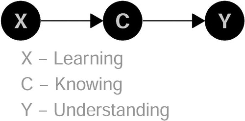
First simulated example: learning (X) effects knowing (C), and knowing causes understanding (Y)—plus some exogenous factors (U, error term). In real life, learning, knowing, and understanding may be operationalized by some questionnaire and standardized for analysis. $$\begin{array}{c}X=U_X,\hspace{1em}{U}_X\sim \mathcal{N}(0,1),\\ C=5·X+U_C,\hspace{1em}{U}_C\sim \mathcal{N}(0,1),\\ Y=3·C+U_Y,\hspace{1em}{U}_Y\sim \mathcal{N}(0,1),\end{array}$$ where $\mathcal{N}(\mu ,\sigma )$ stands for the Normal distribution.

set.seed (1896) # Reproducibility n <- 1000 # Sample Size learning <- rnorm (n) knowing <- 5 * learning + rnorm (n) understanding <- 3 * knowing + rnorm (n)

The corresponding DAG is given in Figure 1.

Fig. 1 DAG for Example 1: Adjusting causes bias.

Without adjustment, the total effect of learning on understanding is unbiased (Equation (1)(1) $$\widehat{y}=-0.022+15.121·x,$$(1) ):

lm1a <- lm (understanding ∼ learning) summary (lm1a){$coefficients[,1:2] ## Estimate Std. Error ## (Intercept) -0.0223 0.0966 ## learning 15.1209 0.0978

Whereas the total effect of learning on understanding is biased downward if adjusted for the covariate (C: knowing, Equation (2)(2) $$\widehat{y}=-0.005+0.122·x+2.982·c.$$(2) ):

lm1b <- lm (understanding ∼ learning + knowing) summary (lm1b) $coefficients[,1:2] ## Estimate Std. Error ## (Intercept) -0.00495 0.0308 ## learning 0.12151 0.1625 ## knowing 2.98174 0.0317 (1) $$\widehat{y}=-0.022+15.121·x,$$(1) (2) $$\widehat{y}=-0.005+0.122·x+2.982·c.$$(2)

Due to the low estimated coefficient of ${\widehat{\beta }}_x=0.122$ with relatively high standard error, mindless multivariate thinking may erroneously conclude that X is not important for modeling Y—but the variables are only conditionally independent given C.

Errors by adjusting for a mediator or post-treatment may not always be so obvious as in this example. In the lab of Cummiskey (2019) who is using a dataset that investigates the effect of teenage smoking on lung function, height is on the causal path between smoking and forced expiratory volume. But adjusting for height would give a downward biased causal effect of smoking and, therefore, not the correct interpretation of the effect of smoking. See Cummiskey et al. (2020) for more details.

3.2 Example 2: Adjusting Removes Bias

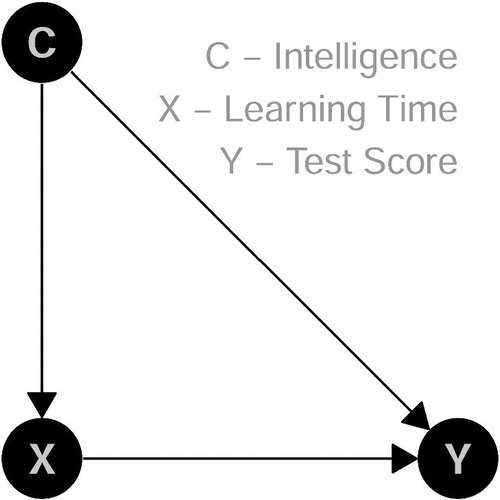
The second simulated example: intelligence (C) reduces learning time (X). Intelligence (C) and learning time (X) cause test score (Y)—plus some exogenous factors (U). Here, we ignore further covariates like motivation or interest and assume a rational and economic student who only studies as many hours X as necessary. $$\begin{array}{c}C=U_C,\hspace{1em}{U}_C\sim \mathcal{N}(100,15),\\ X=200-C+U_X,\hspace{1em}{U}_X\sim \mathcal{N}(0,1),\\ Y=0.5·C+0.1·X+U_Y,\hspace{1em}{U}_Y\sim \mathcal{N}(0,1).\end{array}$$

set.seed(1896) # Reproducibility n <- 1000 # Sample Size intelligence <- rnorm(n, mean = 100, sd = 15) learning.time <- 200 - intelligence + rnorm(n) test.score <- 0.5 * intelligence + 0.1 * learning.time + rnorm(n)

The corresponding DAG is given in Figure 2.

Fig. 2 DAG for Example 2: Adjusting removes bias.

If modeling of the test score would not be adjusted for C (Intelligence), even the sign of the true effect of X (Learning Time) on Y (Test Score) changes—the famous Simpson’s paradox (Simpson 1951) (Equation (3)(3) $$\widehat{y}=100.083-0.401·x,$$(3) ):

lm2a <- lm(test.score ∼ learning.time) summary(lm2a)$coefficients[,1:2] ## Estimate Std. Error ## (Intercept) 100.083 0.23391 ## learning.time -0.401 0.00231

With adjusting the true effect is revealed (Equation (4)(4) $$\widehat{y}=3.446+0.082·x+0.484·c.$$(4) ):

lm2b <- lm(test.score ∼ learning.time + intelligence) summary(lm2b)$coefficients[,1:2] ## Estimate Std. Error ## (Intercept) 3.4465 6.3392 ## learning.time 0.0817 0.0317 ## intelligence 0.4837 0.0317 (3) $$\widehat{y}=100.083-0.401·x,$$(3) (4) $$\widehat{y}=3.446+0.082·x+0.484·c.$$(4)

In this example, without taking the causal structure of the data-generating process into account, one can be puzzled whether the effect of X on Y is positive or negative. Note that this is due to the causal structure of the data generating process. The magnitude and sign of the difference in the estimated coefficients between the adjusted and unadjusted model depends on the true coefficients in the structural causal model (see e.g., Pearl 2013), and may be compared to the Cornfield condition (Cornfield et al. 1959).

In the example of Cummiskey (2019), this situation is given for both covariates age and sex: Both are on the noncausal path between smoking and forced expiratory volume. Not adjusting for them would give wrong results for the causal effect of smoking on forced expiratory volume.

3.3 Example 3: Adjusting Causes Bias

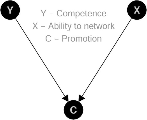
The third simulated example is an example of Berkson’s paradox (Berkson 1946): Ability to network (X) and competence (Y) are independent, promotion (C) depends on both—plus some exogenous factors (see Figure 3). $$\begin{array}{c}X=U_X,\hspace{1em}{U}_X\sim \mathcal{N}(0,1),\\ Y=U_Y,\hspace{1em}{U}_Y\sim \mathcal{N}(0,1),\\ \tilde{C}=\{\begin{array}{cc}1\hfill & \text{if}\mathrm{}\{X>1\vee Y>1\},\hfill \\ 0\hfill & \text{else},\hfill \end{array}\\ C=(1-U_C)·\tilde{C}+U_C·(1-\tilde{C}),\hspace{1em}{U}_C\sim \mathcal{B}(0.05),\end{array}$$ where $\mathcal{B}(\pi )$ stands for the Bernoulli distribution. That is, someone gets promoted—without luck U_C, $\tilde{C}=1$—if the ability to network is high (X > 1) or competence is high (Y > 1).

Fig. 3 DAG for Example 3: Adjusting causes bias.

set.seed(1896) # Reproducibility n <- 1000 # Sample Size network <- rnorm(n) competence <- rnorm(n) promotion <- ((network > 1) | (competence > 1)) luck <- rbinom(n, size = 1, prob = 0.05) promotion <- (1 - luck) * promotion + luck * (1 - promotion)

Note that — is a logical or in R.

Without adjusting for the collider C (i.e., a common outcome of two variables, see, e.g., Elwert 2013), there is only a small, random effect of ability to network (X) on competence (Y) (Equation (5)(5) $$\widehat{y}=-0.006+0.03·x,$$(5) ):

lm3a <- lm(competence ∼ network) summary(lm3a)$coefficients[,1:2] ## Estimate Std. Error ## (Intercept) -0.00581 0.0307 ## network 0.03041 0.0311

But with adjustment for promotion, there seems to be a negative effect (Equation (6)(6) $$\widehat{y}=-0.307-0.14·x+0.957·c.$$(6) ):

lm3b <- lm(competence ∼ network + promotion) summary(lm3b)$coefficients[,1:2] ## Estimate Std. Error ## (Intercept) -0.307 0.0346 ## network -0.140 0.0305 ## promotion 0.957 0.0651 (5) $$\widehat{y}=-0.006+0.03·x,$$(5) (6) $$\widehat{y}=-0.307-0.14·x+0.957·c.$$(6)

Remember that in the data generating process X and Y are causes of C but we mindlessly regressed Y on X. This is especially dangerous if the variable is used as a sampling variable, for example, only those who are promoted are sampled (Equation (7)(7) $$\widehat{y}=0.742-0.313·x.$$(7) ):

lm3c <- lm(competence ∼ network, subset = (promotion == 1)) summary(lm3c)$coefficients[,1:2] ## Estimate Std. Error ## (Intercept) 0.742 0.0644 ## network -0.313 0.0506 (7) $$\widehat{y}=0.742-0.313·x.$$(7)

The reason why this happens can be illustrated by the following example: If you know that someone is promoted (conditional) and you also know that he/she is not good in networking, you know that there is a high probability that he/she is competent—otherwise he/she would not have been promoted.

Here X and Y are independent, but conditionally on C they are dependent—so adjusting C by regression or sampling will generate a spurious correlation between X and Y.

Barrett (2019a) gives an example where income during childhood (which causes education) and genetic risk for diabetes (which causes diabetes in general) cause mother’s diabetes. Therefore, mother’s diabetes is a collider, so adjusting for this would generate a spurious association between education and diabetes.

3.4 Randomized Experiments

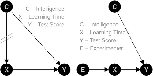
A randomized experiment, here given for the example of Section 3.2 (or an intervention: “do(x)”), erases the arrow into X from the covariable C (left side of Figure 4) as X is manipulated by the experimenter (E) (right side of Figure 4). Instead of letting the necessary learning time (X) depend on intelligence (C) like in subSection 3.2, the learning time is by construction now independent of the covariable. $$\begin{array}{c}C=U_C,\hspace{1em}{U}_C\sim \mathcal{N}(100,15),\\ X=U_X·80+(1-U_X)·120,\hspace{1em}{U}_X\sim \mathcal{B}(0.5),\\ Y=0.5·C+0.1·X+U_Y,\hspace{1em}{U}_Y\sim \mathcal{N}(0,1).\end{array}$$

Fig. 4 DAG for experimental setup in Example 2.

So randomly either do(x) = 80 or do(x) = 120.

set.seed(1896) # Reproducibility n <- 1000 # Sample Size exper.group <- rbinom(n, size = 1, prob = 0.5) learning.time.exper <- exper.group * 80 + (1 - exper.group) * 120 test.score.exper <- 0.5 * intelligence + 0.1 * learning.time.exper + rnorm(n)

The values for intelligence are reused from Section 3.2.

This of course changes the joint distribution, for example, the correlation coefficient r (Equations (8)(8) $$r_{\text{Observational}\mathrm{}\text{Study}}=-0.998,$$(8) and (9)(9) $$r_{\text{Randomized}\mathrm{}\text{Experiment}}=0.015.$$(9) ). Note that we use the R package mosaic (Pruim, Kaplan, and Horton 2017) due to its consistent formula and modeling syntax:

library(mosaic) # Without Experiment cor(intelligence ∼ learning.time) ## [1] -0.998 # With Experiment cor(intelligence ∼ learning.time.exper) ## [1] 0.015 (8) $$r_{\text{Observational}\mathrm{}\text{Study}}=-0.998,$$(8) (9) $$r_{\text{Randomized}\mathrm{}\text{Experiment}}=0.015.$$(9)

But one can also see that randomized experiments balance (observed) covariates (Equations (10)(10) $${\overline{c}}_{do(x)=80}=99.387,$$(10) and (11)(11) $${\overline{c}}_{do(x)=120}=99.832.$$(11) ):

mean (intelligence ∼ learning.time.exper) ## 80 120 ## 99.4 99.8 (10) $${\overline{c}}_{do(x)=80}=99.387,$$(10) (11) $${\overline{c}}_{do(x)=120}=99.832.$$(11)

Moreover, now the effect of X on Y is an unbiased estimate—without adjusting for C (Equation (12)(12) $$\widehat{y}=49.079+0.107·x,$$(12) , compare Equation (3)(3) $$\widehat{y}=100.083-0.401·x,$$(3) ):

lm4a <- lm(test.score.exper ∼ learning.time.exper) summary(lm4a)$coefficients[,1:2] ## Estimate Std. Error ## (Intercept) 49.079 1.2005 ## learning.time.exper 0.107 0.0118or with adjusting (Equation (13)(13) $$\widehat{y}=-0.029+0.102·x+0.499·c.$$(13) , compare Equation (4)(4) $$\widehat{y}=3.446+0.082·x+0.484·c.$$(4) ):

lm4b <- lm(test.score.exper ∼ learning.time.exper + intelligence) summary(lm4b)$coefficients[,1:2] ## Estimate Std. Error ## (Intercept) -0.0286 0.26206 ## learning.time.exper 0.1017 0.00156 ## intelligence 0.4986 0.00211 (12) $$\widehat{y}=49.079+0.107·x,$$(12) (13) $$\widehat{y}=-0.029+0.102·x+0.499·c.$$(13)

The effect of intelligence can be estimated unconditionally (Equation (14)(14) $$\widehat{y}=9.924+0.501·c.$$(14) ):

lm4c <- lm(test.score.exper ∼ intelligence) {summary(lm4c)$coefficients[,{1:2] ## Estimate Std. Error ## (Intercept) 9.924 0.48682 ## intelligence 0.501 0.00483 (14) $$\widehat{y}=9.924+0.501·c.$$(14)

Thinking about randomized experiments in this way (and showing the simulated example) can help to understand why randomized experiments can succeed and why some claim “No causation without manipulation” (e.g., Holland 1986).

3.5 Extensions

In a similar way, the different outcomes of observing or intervention as well as counterfactual evaluations can be made accessible (compare Section 2).

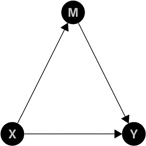
If limited to the linear case, also mediation analysis (total, direct, and indirect effects) can be shown coherently—with M being a mediator variable like in Figure 5.

Fig. 5 DAG for mediation analysis.

The simulated examples are meant to be introduced as illustrational material in introductory classes.

Of course, there is much more to discuss in causal inference than shown here, like, for example, backdoor and frontdoor criteria, depending on time and prior knowledge of students.

3.6 Remarks

Also, it should be remembered and addressed in class that these causal thoughts are not mandatory on the first level (Pearl 2019), that is, if one is only interested in the associations (and predictions within). However, this narrow view on the use of data may limit the perceived power of statistics and data science (Rossman and Witmer 2019) in the eye of the students (compare Schield 2018).

We adapted the real life example by Cummiskey (2019) in a learnr (Schloerke, Allaire, and Borges 2019) tutorial (in German), accessible under the following link: https://fomshinyapps.shinyapps.io/KausaleInferenz/.

4 Discussion

We concur with Wild et al. (2017):

With the rapid, ongoing expansions in the world of data, we need to devise ways of getting more students much further, much faster.

We think that statistical education, with help of technological innovations, improved a lot: Simulation based inference, focus on multivariate modeling, and reproducible analysis are certainly steps forward. But in statistics and data science there are still far too many misconceptions and analytic flaws. By the given, very simple examples, we try to help students to see the dangers and opportunities in understanding something about the real world by our models. The substantive correctness of the model results does not need to be discovered by the quantitative statistical model alone, like, for example, p-values, AIC, or $R_{\text{adj}}^2$. As anecdotal evidence: while presenting the examples, even senior researchers report that these helped them to think more clearly about association and causality. By illustrating causal inference by means of the workhorse linear modeling and changing the curriculum (Cobb 2015) we hope to “best prepare [students] for and keep pace with this data-driven era of tomorrow” (National Academies of Sciences, Engineering, and Medicine 2018).

Of course, the use of simulated, linear data with only three variables (X, Y, C) is very limited and far from real and complex. But if we—and our students—do not understand these simple cases, how sure can we be that any of us will ask the right questions and draw the right conclusions in big data situations?

Acknowledgments

We like to thank Amy Wehe for her language support. The remarks of three anonymous reviewers and the editors helped to improve this article a lot.

References

- Angrist, J. D., and Pischke, J.-S. (2014), Mastering’Metrics: The Path From Cause to Effect, Princeton, NJ: Princeton University Press.
- Barrett, M. (2019a), “Common Structures of Bias,” available at https://ggdag.netlify.com/articles/bias-structures.html.
- Barrett, M. (2019b), “ggdag: Analyze and Create Elegant Directed Acyclic Graphs,” R Package Version 0.2.0, available at https://CRAN.R-project.org/package=ggdag.
- Berkson, J. (1946), “Limitations of the Application of Fourfold Table Analysis to Hospital Data,” Biometrics Bulletin, 2, 47–53. DOI: 10.2307/3002000.
- Cobb, G. W. (2015), “Mere Renovation Is Too Little Too Late: We Need to Rethink Our Undergraduate Curriculum From the Ground Up,” The American Statistician, 69, 266–282, DOI: 10.1080/00031305.2015.1093029.
- Cornfield, J., Haenszel, W., Hammond, E. C., Lilienfeld, A. M., Shimkin, M. B., and Wynder, E. L. (1959), “Smoking and Lung Cancer: Recent Evidence and a Discussion of Some Questions,” Journal of the National Cancer Institute, 22, 173–203.
- Cummiskey, K. (2019), “Causal Inference in Introductory Statistics Courses,” available at https://github.com/kfcaby/causalLab.
- Cummiskey, K., Adams, B., Pleuss, J., Turner, D., Clark, N., and Watts, K. (2020), “Causal Inference in Introductory Statistics Courses,” Journal of Statistics Education, DOI: 10.1080/10691898.2020.1713936.
- Elwert, F. (2013), “Graphical Causal Models,” in Handbook of Causal Analysis for Social Research, ed. S. Morgan, Dordrecht: Springer, pp. 245–273.
- Gelman, A., and Hill, J. (2012), Data Analysis Using Regression and Multilevel/Hierarchical Models, New York: Cambridge University Press.
- Gould, R. (2017), “Data Literacy Is Statistical Literacy,” Statistics Education Research Journal, 16, 22–25.
- Hardin, J., Hoerl, R., Horton, N. J., Nolan, D., Baumer, B., Hall-Holt, O., Murrell, P., Peng, R., Roback, P., Lang, D. T., and Ward, M. D. (2015), “Data Science in Statistics Curricula: Preparing Students to ‘Think With Data’,” The American Statistician, 69, 343–353, DOI: 10.1080/00031305.2015.1077729.
- Hernán, M. A., Hsu, J., and Healy, B. (2019), “A Second Chance to Get Causal Inference Right: A Classification of Data Science Tasks,” CHANCE, 32, 42–49, DOI: 10.1080/09332480.2019.1579578.
- Holland, P. W. (1986), “Statistics and Causal Inference,” Journal of the American statistical Association, 81, 945–960. DOI: 10.1080/01621459.1986.10478354.
- Imbens, G. W., and Rubin, D. B. (2015), Causal Inference in Statistics, Social, and Biomedical Sciences, Cambridge: Cambridge University Press.
- Jamie, D. M. (2002), “Using Computer Simulation Methods to Teach Statistics: A Review of the Literature,” Journal of Statistics Education, 10, 1–20. DOI: 10.1080/10691898.2002.11910548.
- Kaplan, D. (2011), Statistical Modeling: A Fresh Approach (2nd ed.), Project MOSAIC Books. Retrieved from http://project-mosaic-books.com/
- Kaplan, D. (2018), “Teaching Stats for Data Science,” The American Statistician, 72, 89–96, DOI: 10.1080/00031305.2017.1398107.
- Lindeløv, J. K. (2019), “Common Statistical Tests Are Linear Models (or: How to Teach Stats),” available at https://lindeloev.github.io/tests-as-linear/.
- Morgan, S. L., and Winship, C. (2015), Counterfactuals and Causal Inference (2nd ed.), Cambridge: Cambridge University Press.
- National Academies of Sciences, Engineering, and Medicine (2018), Data Science for Undergraduates: Opportunities and Options, Washington, DC: The National Academies Press, DOI: 10.17226/25104.
- Pearl, J. (2013), “Linear Models: A Useful ‘Microscope’ for Causal Analysis,” Journal of Causal Inference, 1, 155–170. DOI: 10.1515/jci-2013-0003.
- Pearl, J. (2019), “The Seven Tools of Causal Inference, With Reflections on Machine Learning,” Communications of the ACM, 62, 54–60.
- Pearl, J., Glymour, M., and Jewell, N. P. (2016), Causal Inference in Statistics: A Primer, Chichester: Wiley.
- Pearl, J., and Mackenzie, D. (2018), The Book of Why: The New Science of Cause and Effect, New York: Basic Books.
- Peters, J., Janzing, D., and Schölkopf, B. (2017), Elements of Causal Inference: Foundations and Learning Algorithms, Cambridge, MA: MIT Press.
- Pruim, R., Kaplan, D., and Horton, N. (2017), “The Mosaic Package: Helping Students to ‘Think With Data’ Using R,” The R Journal, 9, 77–102, DOI: 10.32614/RJ-2017-024.
- R Core Team (2019), R: A Language and Environment for Statistical Computing, Vienna, Austria: R Foundation for Statistical Computing, available at https://www.R-project.org/.
- Ridgway, J. (2016), “Implications of the Data Revolution for Statistics Education,” International Statistical Review, 84, 528–549, DOI: 10.1111/insr.12110.
- Rossman, A., and De Veaux, R. (2016), “Interview With Richard De Veaux,” Journal of Statistics Education, 24, 157–168, DOI: 10.1080/10691898.2016.1263493.
- Rossman, A. J., and Witmer, J. (2019), “Interview With Jeff Witmer,” Journal of Statistics Education, 27, 48–57, DOI: 10.1080/10691898.2019.1603506.
- Schield, M. (2018), “Confounding and Cornfield: Back to the Future,” in Looking Back, Looking Forward. Proceedings of the Tenth International Conference on Teaching Statistics, eds. M. A. Sorto, A. White, and L. Guyot, available at http://www.statlit.org/pdf/2018-Schield-ICOTS.pdf.
- Schloerke, B., Allaire, J. J., and Borges, B. (2019), “learnr: Interactive Tutorials for R,” R Package Version 0.10.0, available at https://CRAN.R-project.org/package=learnr.
- Simpson, E. H. (1951), “The Interpretation of Interaction in Contingency Tables,” Journal of the Royal Statistical Society, Series B, 13, 238–241. DOI: 10.1111/j.2517-6161.1951.tb00088.x.
- Stark, P. B., and Saltelli, A. (2018), “Cargo-Cult Statistics and Scientific Crisis,” Significance, 15, 40–43, DOI: 10.1111/j.1740-9713.2018.01174.x.
- Steel, E. A., Liermann, M., and Guttorp, P. (2019), “Beyond Calculations: A Course in Statistical Thinking,” The American Statistician, 73, 392–401, DOI: 10.1080/00031305.2018.1505657.
- Wild, C. J., Pfannkuch, M., Regan, M., and Parsonage, R. (2017), “Accessible Conceptions of Statistical Inference: Pulling Ourselves Up by the Bootstraps,” International Statistical Review, 85, 84–107, DOI: 10.1111/insr.12117.
- Wood, B. L., Mocko, M., Everson, M., Horton, N. J., and Velleman, P. (2018), “Updated Guidelines, Updated Curriculum: The Gaise College Report and Introductory Statistics for the Modern Student,” CHANCE, 31, 53–59, DOI: 10.1080/09332480.2018.1467642.