Sensitivity Analysis of the No-Omitted Confounder Assumption in Latent Growth Curve Mediation Models

Abstract

Latent growth curve mediation models are increasingly used to assess mechanisms of behavior change. For latent growth mediation model, like any another mediation model, even with random treatment assignment, a critical but untestable assumption for valid and unbiased estimates of the indirect effects is that there should be no omitted variable that confounds indirect effects. One way to address this untestable assumption is to conduct sensitivity analysis to assess whether the inference about an indirect effect would change under varying degrees of confounding bias. We developed a sensitivity analysis technique for a latent growth curve mediation model. We compute the biasing effect of confounding on point and confidence interval estimates of the indirect effects in a structural equation modeling framework. We illustrate sensitivity plots to visualize the effects of confounding on each indirect effect and present an empirical example to illustrate the application of the sensitivity analysis.

Keywords:

• correlated augmented model
• indirect effect
• latent growth curve
• Multiple mediation analysis
• sensitivity analysis

Mediation analysis assesses the effect of a treatment (independent) variable on an outcome variable via one or more mediators measured sequentially over time (MacKinnon, 2008). Complex multiple mediation models have become more common (e.g., Alvarez & Juang, 2010; Z. Chen & Wang, 2017; Demiray & Janssen, 2015; Kershaw, Mezuk, Abdou, Rafferty, & Jackson, 2010; Ma, Cheng, Ribbens, & Zhou, 2013; Priesemuth, Schminke, Ambrose, & Folger, 2014; Strelan, Karremans, & Krieg, 2017; Villegas-Gold & Yoo, 2014). In the current paper, we focus on a mediation model with two covarying (parallel) mediators where the term “parallel” indicates that there is no direct causal path between the two mediators. One important application of a multiple mediator model with two covarying mediators is the latent growth curve mediation model (LGCMM) with repeated measures/multilevel data, whereby some treatment variable is expected to affect an outcome via the change in some mediating process (Selig & Preacher, 2009; Von Soest & Hagtvet, 2011). LGCMM is increasingly used to test hypothesized mechanisms of behavior change following treatments for psychological disorders (Hallgren, Wilson, & Witkiewitz, 2018). For example, as shown in Figure 1, in alcohol treatment one might hypothesize that an anti-craving medication (e.g., naltrexone) affects reductions in alcohol use via changes in craving over time. Such a model would require estimation of two separate indirect effects: the indirect effect of treatment on alcohol use through the intercept of craving and the indirect effect of treatment on alcohol use through the slope of craving. In addition, LGCMM accounts for inter-dependencies of repeated measures data for the same individuals over time for the mediator and outcome variables.¹

Figure 1 Latent growth mediation model. Indirect effect of intervention (naltrexone vs. non-naltrexone) treatment on percent drinking days at week 16 is assumed to be mediated via latent intercept (mean alcohol craving in week 4) and weekly growth rate of alcohol craving. The percent drinking days is divided by 10 to make its dispersion smaller and more comparable to rest of the data. For the indirect effect involving latent intercept, B (SE) = −0.227 (0.073), 97.5% CI [−0.398, −0.067]; for the indirect effect involving latent slope, B (SE) = 0.01 (0.094), 97.5% CI [−0.206, 0.227]. A solid straight arrow shows the effect of a variable at the origin on the variable at the end of the arrow. A solid double-headed curved arrow shows covariance between two variables. Observed variables associated with the latent intercept and slopes are excluded for simplicity.

Like any statistical model, a mediation model must meet certain assumptions to produce valid and unbiased estimates (James & Brett, 1984; Judd & Kenny, 1981; MacKinnon, 2008; Robins & Greenland, 1992). We focus on a widely acknowledged limitation of the mediation model, the assumption of no omitted confounders, which is necessary to produce unbiased, causally interpretable estimates of the indirect effect (Imai, Keele, & Tingley, 2010; Judd & Kenny, 1981; MacKinnon & Pirlott, 2015; Pearl, 2014; Robins & Greenland, 1992; Valente, Pelham, Smyth, & MacKinnon, 2017). When the independent variable is a random treatment assignment, this assumption states that there should be no omitted confounder variable that influences any pair of endogenous variables, that is, the mediator(s) and outcome(s). Unfortunately, this assumption is not testable (Holland, 1988). When designing a study, researchers usually include all the relevant variables that are hypothesized to influence the mediator(s) and the outcome variable(s). However, there are cases when the substantive theory is incomplete, it is unrealistic or impossible to measure all relevant variables, or a researcher analyzes an archival data set that does not include all theoretically relevant variables. Because it is typically impossible to randomize levels of the mediators to different participants, it is typically impossible to rule out the potential impact of omitted confounders on the relationships between the mediator(s) and outcome variables. It is thus recommended that one conduct a sensitivity analysis to ascertain the biasing effects of potential omitted confounders on the model estimates, including point and interval estimates of the indirect affect (Cox, Kisbu-Sakarya, Miočević, & MacKinnon, 2013; Imai, Keele, & Yamamoto, 2010; MacKinnon & Pirlott, 2015; Tofighi & Kelley, 2016; VanderWeele, 2010).

For single-level data (data that are not grouped or repeated measures), previous studies addressed sensitivity analysis for (a) single mediator model, an example of which is depicted in Figure 2 (Cox et al., 2013; Imai et al., 2010; Valente et al., 2017; VanderWeele, 2010); (b) multiple mediator model with two mediators that were assumed to be independent, which makes a strong causal assumption about independence of the two mediators (Imai & Yamamoto, 2013); and (c) multiple mediator model with the mediators assumed to be sequentially related (Daniel, De Stavola, Cousens, & Vansteelandt, 2015; Harring, McNeish, & Hancock, 2017). To the best of our knowledge, no study has extended sensitivity analysis to a longitudinal mediation model with two covarying mediators. The existence of two covarying mediators adds an additional complexity in computing indirect effects and conducting sensitivity analysis compared to a single mediator model. Analyzing each mediator one at a time could lead to biased estimates of indirect effects even when the two mediators are assumed to be independent (VanderWeele, 2015). A confounder may affect two relationships between each of the mediators and the outcome variable as opposed to one effect of the mediator on the outcome variable in a single mediator model. The effect of a potential confounder on the two relationships between the mediators and the outcome variable across two parallel mediation processes is likely to be differential, thus making modeling potential confounding bias more challenging. Thus, techniques developed for a single mediator model cannot directly be applied to a multiple mediator model.

Figure 2 A general single mediator model. All the variables can be observed or latent. X, M, and Y denotes antecedent, mediator, and outcome variable, respectively. U denotes one or more omitted confounders. C denotes one or more covariates (e.g., background variables) included in the model. We assume that C is measured before X, which is measured before M, and which is measured before Y. A solid arrow shows the effect of a variable at the origin on the variable at the end of the arrow. A dashed double-headed curved arrow illustrates a confounder correlation (covariance) between U and another variable in the model.

For the LGCMM in Figure 1, we are interested in the two Between indirect effects through two covarying latent intercept and slope. None of the previous studies have extended sensitivity analysis to a longitudinal model with two covarying latent mediators. As mentioned before, applying single-mediator sensitivity techniques to a two-mediator model is likely to produce biased results and thus is not recommended (VanderWeele, 2015). Using multilevel structural equation modeling (SEM) framework, Tofighi and Kelly (2016) proposed a post-hoc method to compute the omitted confounder effect on the point estimate of the indirect effect but did not offer a method to compute standard errors and CIs for adjusted indirect effects. Using the potential outcomes framework (Rubin, 1974, 1978), Talloen et al. (2016) used fixed-effect techniques (Allison, 2005) to remove the confounding bias at the Between level and thus relax the assumption of no omitted confounder at the Between level. The fixed-effect technique cannot be applied to LGCMM in our study because the fixed-effect technique removes all the Between variability (McNeish & Kelley, 2018), which is the focus of our study. In related work, Bind, VanderWeele, Coull, and Schwartz (2016) extended the potential outcomes framework to define indirect effects for a single mediator with longitudinal data; however, they did not propose a method to conduct sensitivity analysis. Moreover, techniques developed for single-level data where the observations are assumed to be independent cannot directly be applied in a longitudinal growth context without additional analytic work to account for correlated observations (Tofighi & Kelley, 2016). Multilevel data pose additional challenges in determining whether mediation occurs at Between, Within, or cross levels (Bind et al., 2016; Tofighi & Kelley, 2016; Tofighi, West, & MacKinnon, 2013).

Our manuscript provides tools to help applied users conduct sensitivity analysis for an LGCMM with commonly used measures of effect sizes. We extend sensitivity analysis to LGCMM with two covarying latent growth factors in an SEM framework. We propose a technique termed correlated augmented model sensitivity analysis (CAMSA) to conduct sensitivity analysis. This technique, which is based on an SEM framework, uses a correlated augmented model. We proposed the correlated augmented model to prevent the negative residual variance problem of using latent proxy (phantom) variable techniques (Harring et al., 2017; Tofighi & Kelley, 2016), in which we reparametrized the model with a latent proxy variable technique when conducting sensitivity analysis. Reparameterization of an SEM has been suggested as a method to prevent negative residual variance, although not in the sensitivity analysis context (Rindskopf, 1983). The proposed CAMSA augments the mediation model with additional covariances between residuals associated with endogenous variables, termed confounder covariances, to model the effect of the potential confounders. We offer analytic results to use confounder covariances to compute correlation between the residuals, termed sensitivity parameters (Imai et al., 2010). Because sensitivity parameters are confounder correlations, they offer an intuitive way to quantify the magnitude of confounding bias in terms of effect sizes. We also compute effect sizes for confounding effects in terms of the squared (semi-) partial correlations, which determine unique effect sizes due to the confounder. We present analytic results showing how the confounder correlations (sensitivity parameters) are used to estimate confounding biases, thereby modeling confounding effects. We also discuss strengths and weaknesses of CAMSA. We then use an empirical example to show how CAMSA can be conducted in Mplus (L. K. Muthén & Muthén, 2017). We also present two sets of graphs to visualize the results of the sensitivity analysis for each mediation process.

CAUSAL ASSUMPTIONS IN LATENT GROWTH CURVE MEDIATION MODELING

In this section, we examine the causal inference assumptions necessary to produce an interpretable causal estimate of the indirect effect in an LGCMM. First, to clarify the no omitted confounder assumption, we consider a randomized experiment single mediation model in which X denotes a properly executed random assignment to two levels of a treatment. Because X denotes random assignment, we can rule out the following confounding effects: C → X and X → C, given the relationships between X and the covariates (C) can be assumed to be zero because proper randomization balances out potential pre-treatment differences on the pre-treatment variables measured in C. Finally, when X is randomized, the X → M effect is not confounded by omitted variables (Holland, 1988). However, randomized assignment cannot rule out the following confounding effects. First, X → U effect, the confounder can be caused by X and cannot automatically be assumed zero because U is a post-treatment variable. Second, the effect of U on the M → Y relationship may not be ruled out. Thus, when the no-omitted confounder assumption is violated, the M → Y and X → Y effects in Figure 2 are potentially confounded by an unmeasured variable (Imai et al., 2010; Judd & Kenny, 1981; MacKinnon, 2008; Pearl, 2011; 2014; Robins & Greenland, 1992; VanderWeele, 2010).

Extension of the no-confounder assumption to a multilevel single mediator model has been discussed in the literature (Bind et al., 2016; Talloen et al., 2016; Tofighi & Kelley, 2016) We discuss extension of the no omitted confounder assumption to the LGCMM in Figure 1. Given that the hypothesized LGCMM has a randomized intervention (X), the no omitted confounder assumption is satisfied if the following two assumptions hold. (1) For each person, there should not be an omitted confounder that influences a pair of variables that include the two mediators as well as the outcome variable. (2) An omitted confounder should not be influenced by X. As mentioned previously, even for randomized intervention X, we cannot be certain Assumption 1 holds, thus we should conduct sensitivity analysis. For the LGCMM model in the empirical example, however, we can assume that the randomized trial does not affect an omitted confounder that, in turn, affects the mediators and outcome variables. This is because in our substantive example, the intervention was specifically designed to manipulate alcohol craving. However, existence of a confounder U that is affected by X would imply that U is another mediator that is missing from the model. Given that X was randomized, and the treatment was specifically designed to reduce craving, we can rule out that X does not impact any additional intermediate variable. Finally, given X is randomized, we can rule out the effect of an omitted confounder on the mediators. Taken together, multiple mediators (intercept and slope of the LGCMM) adds more complexity for conceptualizing potential confounders because there can be more patterns of confounding relationships compared to the single mediator model.

PROPOSED SENSITIVITY ANALYSIS METHOD FOR LGCMM

In the next section, we specify two equivalent augmented models to compute the effect of omitted confounders. The analytic results will be used to conduct sensitivity analysis for a mediation model with two covarying mediators and one outcome variable. We use LGCMM to derive the results. Later, we discuss strengths and limitations of the results in terms of their application to different mediation models with two covarying mediators that are either latent or observed. The first model is termed the latent augmented model. This technique, which is based on SEM framework, is an extension of a sensitivity analysis method for a single mediator model in multilevel SEM (Tofighi & Kelley, 2016), as well as phantom variable sensitivity analysis in single-level SEM (Harring et al., 2017). The second model is termed the correlated augmented model that uses correlations between residuals of the endogenous variables, termed confounder correlations (sensitivity parameters), to model the effect of the omitted confounder. As will be discussed later, the correlated augmented model has an advantage of not using a phantom variable, a latent variable without indicators, which could cause a negative residual variance.

LATENT AUGMENTED MODEL

In the latent augmented model, which is an extension of the sensitivity analysis proposed by Tofighi and Kelley (2016) and Harring et al. (2017), we first introduce a latent proxy (phantom) variable $\varpi$ (a latent variable with no indicators), which represents all potential confounders into the model. This model is termed the latent augmented model. This latent proxy variable may represent one or more omitted confounders that are assumed to be linearly related to all endogenous variables in the model. Figure 3 shows the augmented LGCMM model. The dashed circle shows the latent proxy (phantom) variable ϖ and dashed arrows show unknown confounding effects on the mediators (latent intercept and slope) and the outcome variable. We term these coefficients as the confounder parameters. For identification purposes, the latent proxy variable is assumed to have a standard normal distribution (Tofighi & Kelley, 2016). The confounder parameters are set to values determining the degrees of confounding between the latent proxy variable and the endogenous variables (two latent variables and the outcome variable) in the model.

Figure 3 Latent augmented model. Indirect effect of intervention (naltrexone vs. placebo) treatment on percent drinking days at week 16 is assumed to be mediated via latent intercept (mean alcohol craving at week 4) and weekly growth rate of alcohol craving from weeks 6 through 12.

The following equations specify the latent augmented model. We use subscript “*” to denote the model parameters and residuals in the augmented model:

(1) $m_{ij}={\eta }_{i0}+{\eta }_{i1}{t}_{ij}+e_{ij}^{\ast }$(1)

(2) ${\eta }_{i0}={\alpha }_0^{\ast }+{\gamma }_{01}^{\ast }{x}_i+{\gamma }_{02}^{\ast }{\varpi }_i+{\zeta }_{0i}^{\ast }$(2)

(3) ${\eta }_{i1}={\alpha }_1^{\ast }+{\gamma }_{11}^{\ast }{x}_i+{\gamma }_{12}^{\ast }{\varpi }_i+{\zeta }_{1i}^{\ast }$(3)

(4) $y_i={\nu }^{\ast }+{\kappa }^{\ast }{x}_i+{\lambda }_1^{\ast }{\eta }_{i0}+{\lambda }_2^{\ast }{\eta }_{i1}+{\lambda }_3^{\ast }{\varpi }_i+{\epsilon }_i^{\ast }$(4)

where the subscript i denotes a person i = 1, …, N, subscript j denotes an occasion, j = 1,…, p. The variables $m_{ij}$ and $t_{ij}$ denote the mediator (e.g., craving) and time score (e.g., week) for person i at occasion j, respectively; $y_i$and $x_i$ denote the distal (ultimate) outcome (alcohol use) and random treatment assignment, respectively. The growth factors for the augmented LGCMM are denoted by ${\eta }_{i0}$ for the intercept, describing person’s latent score at the time score of 0 (e.g., mean craving in week 4), and ${\eta }_{i1}$ for the latent slope, describing a person’s latent rate of change in the mediator (e.g., weekly change in craving) over time; ${\alpha }_0^{\ast }$ and ${\alpha }_1^{\ast }$ denote the intercepts for the latent growth factors and ${\nu }^{\ast }$denotes the intercept for the distal outcome; ${\gamma }_{01}^{\ast }$, ${\gamma }_{11}^{\ast }$, and ${\kappa }^{\ast }$ quantify direct treatment effects on the latent intercept and slope and the distal outcome variable, respectively; ${\lambda }_1^{\ast }$ and ${\lambda }_2^{\ast }$ quantify the effect of the latent intercept and slope on the distal outcome variable, respectively. Confounder coefficients are the effects of ϖ on the latent intercept, slope, and the outcome variable, denoted by ${\gamma }_{02}^{\ast }$, ${\gamma }_{12}^{\ast }$, and ${\lambda }_3^{\ast }$, respectively. The confounder parameters, ${\gamma }_{02}^{\ast }$, ${\gamma }_{12}^{\ast }$, and ${\lambda }_3^{\ast }$, must be fixed to make the model identified for estimation purposes.

For the augmented model, the vector of residuals is denoted by ${\epsilon }^{\ast }={\left({\mathbf{e}}^{\ast },{\epsilon }_i^{\ast },{\zeta }_{0i}^{\ast },{\zeta }_{1i}^{\ast }\right)}^{\mathrm{T}}$, where ${\mathbf{e}}^{\ast }={\left(e_{i1}^{\ast },\dots ,e_{ip}^{\ast }\right)}^{\mathrm{T}}$is the vector of residuals for $m_{ij}$s, and T denotes vector transpose operator. It should be noted that ϖ is an exogenous latent variable without a residual term (i.e., residual term equals zero) and thus is not included in the residual vector. Given ϖ and $\mathit{x}$ , the vector of residuals has a multivariate normal distribution with mean vector of zeros,${\epsilon }_i^{\ast }\sim \mathcal{N}\left(0,{\mathbf{\Psi }}^{\ast }\right),$ and the following covariance matrix:

where ${\mathbf{\Psi }}_{{\mathbf{e}}^{\ast }}$ is the covariance matrix of ${\mathbf{e}}^{\ast }$. When all confounders are included in the model, it can be shown that the residuals associated with mediators and outcome variables are uncorrelated under certain additional assumptions (Tofighi & Kelley, 2016; Tofighi et al., 2013). This means that residuals associated with the outcome variable ${\epsilon }_i^{\ast }$ are not correlated with the residuals associated with latent factors, ${\zeta }^{\ast }$s. It should be noted that, however, ${\zeta }^{\ast }$s, are usually assumed to covary in multilevel and longitudinal analysis literature (Grimm, Ram, & Estabrook, 2017; Singer & Willett, 2003; Snijders & Bosker, 2011). This covariance can be of substantive interest because the status for an individual at time zero (intercept) can be related to the person’s rate of growth (slope). However, we should emphasize that in the augmented model this covariance may not be solely due to an omitted confounder. In other words, if this covariance is a result of an omitted confounder, then this covariance is already modeled by ϖ, which is assumed to represent all the omitted confounders. As shown below, given $\mathit{x}$ the covariance between the growth factors is decomposed into two parts:

(5) $\mathrm{c}\mathrm{o}\mathrm{v}\left({\eta }_{i0},{\eta }_{i1}|\mathit{x}\right)={\gamma }_{02}^{\ast }{\gamma }_{12}^{\ast }{\sigma }_{\varpi }^2+{\sigma }_{{\zeta }_0^{\ast },{\zeta }_1^{\ast }},$(5)

where ${\sigma }_{{\zeta }_0^{\ast },{\zeta }_1^{\ast }}=\mathrm{c}\mathrm{o}\mathrm{v}({\zeta }_{i1}^{\ast },{\zeta }_{i2}^{\ast }|\mathit{x})$. In the above equation, the first term ${\sigma }_{\varpi }^2{\gamma }_{02}^{\ast }{\gamma }_{12}^{\ast }$ quantifies the confounding part of the covariance between the growth factors due to ϖ and the term ${\sigma }_{{\zeta }_0^{\ast },{\zeta }_1^{\ast }}$specifies the non-confounding part of the covariance. Similarly, we can derive the covariance between ${\eta }_{i0}$ and ${\eta }_{i1}$ and ϖ:

(6) $\mathrm{c}\mathrm{o}\mathrm{v}\left({\eta }_{i0},{\varpi }_i|\mathit{x}\right)={\gamma }_{02}^{\ast }{\sigma }_{\varpi }^2,$(6)

(7) $\mathrm{c}\mathrm{o}\mathrm{v}\left({\eta }_{i1},{\varpi }_i|\mathit{x}\right)={\gamma }_{12}^{\ast }{\sigma }_{\varpi }^2,$(7)

More succinctly, the conditional covariance matrix between the vector of latent variables,${\eta }_i^{\ast }={\left({\eta }_{i0},{\eta }_{i1},{\varpi }_i\right)}^{\mathrm{T}}$, is as follows:

(8) $\mathrm{c}\mathrm{o}\mathrm{v}({\eta }_i^{\ast }|x)={\sigma }_{\varpi }^2\left[\begin{array}{c}{\left({\gamma }_{02}^{\ast }\right)}^2+{\sigma }_{{\zeta }_0^{\ast }}^2{\gamma }_{02}^{\ast }{\gamma }_{12}^{\ast }+{\sigma }_{{\zeta }_0^{\ast },{\zeta }_1^{\ast }}{\gamma }_{02}^{\ast }\\ {\gamma }_{02}^{\ast }{\gamma }_{12}^{\ast }+{\sigma }_{{\zeta }_0^{\ast },{\zeta }_1^{\ast }}{\left({\gamma }_{12}^{\ast }\right)}^2+{\sigma }_{{\zeta }_1^{\ast }}^2{\gamma }_{12}^{\ast }\\ {\gamma }_{02}^{\ast }{\gamma }_{12}^{\ast }1\end{array}\right]$(8)

To compute the indirect effect in the augmented model, we introduce different levels of confounding bias by manipulating values of the confounding parameters. The confounding parameters take on various values influencing the latent intercept and slope and the outcome variable. We need to identify different values for the confounder parameters that are of substantive interest for two reasons. First, note that because the mediators and outcome variables are not standardized, the parameter values depend on the metric of the variables. Second, we need computational formulas that would translate a researcher’s knowledge about the range of correlation values to confounder parameters. To make the choice of the values for the parameters more intuitive, we compute the confounder parameter values as a function of the correlation values which are more understandable. The correlation values, termed confounder correlations (sensitivity parameters), can be used to compute effect sizes of confounding effects in terms of the squared (semi-)partial correlations, which determine unique effect sizes due to the confounder. That is, we first determine a set of plausible values (e.g., correlation values based on prior research if any exists or other information) for confounder correlations and then compute the confounder parameter values. Given that ϖ and x are not correlated and variance of ϖ is one, we have

(9) ${\gamma }_{02}^{\ast }={\sigma }_{{\eta }_0}{\rho }_{{\eta }_0,\varpi }$(9)

(10) ${\gamma }_{12}^{\ast }={\sigma }_{{\eta }_1}{\rho }_{{\eta }_1,\varpi }$(10)

(11) ${\lambda }_3^{\ast }={\sigma }_y{\rho }_{y,\varpi }-{\lambda }_1^{\ast }{\gamma }_{02}^{\ast }-{\lambda }_2^{\ast }{\gamma }_{12}^{\ast }$(11)

where ${\rho }_{{\eta }_0,\varpi }$, ${\rho }_{{\eta }_1,\varpi }$, and ${\rho }_{y,\varpi }$ denote confounder correlations between the latent proxy variable and latent intercept and slope and the outcome variable, respectively. These correlations take on a combination of the values set by the researcher. The parameters, ${\sigma }_{{\eta }_0}$, ${\sigma }_{{\eta }_1}$, and ${\sigma }_y$ are the population standard deviations for the latent intercept, latent slope and outcome variable, respectively. We can estimate the variance of the growth factors (${\sigma }_{{\eta }_0}^2$ and ${\sigma }_{{\eta }_1}^2$) from the latent growth model where there are no predictors (i.e., $\mathit{x}$ and C) or the outcome variable (y) in the model; ${\sigma }_y$is estimated by calculating the sample standard deviation.

Unfortunately, the latent augmented model (as specified in Figure 3) can result in a negative residual variance (i.e., Heywood cases; Dillon, Kumar, & Mulani, 1987; Kolenikov & Bollen, 2012; Rindskopf, 1984). For our empirical example, the latent augmented LGCMM produced a negative variance estimate regardless of the values of sensitivity parameters. The Heywood case for an augmented LGCMM is likely to occur because fitting a phantom variable that is not supported by data is likely to cause negative residual variance. As Bartholomew, Knott, and Moustaki (2011) point out,

One of the commonest cause of Heywood cases is the attempt to extract more factors than are present. This is readily demonstrated by simulation but might have been anticipated on the grounds that artificially inflating the communality forces the residuals towards zero. (p. 67)

CORRELATED AUGMENTED MODEL SENSITIVITY ANALYSIS

To prevent the Heywood case associated with estimation of the latent augmented model, we propose the CAMSA. CAMSA uses the correlated augmented model² shown in Figure 4, which is equivalent (i.e., has the same likelihood function; Kreft, De Leeuw, & Aiken, 1995) to the latent augmented model in Figure 3. That is, we reparametrize the latent augmented model to create the correlated augmented model that does not use a latent proxy (phantom) variable and thus avoids a potential Heywood case (i.e., negative residual variance). Although not in the context of sensitivity analysis, previous research suggested using reparameterization to prevent Heywood cases (Rindskopf, 1983). Because the two models, the reparametrized model and the original model, are equivalent, the reparametrized model parameters are a function of the parameters in the original model. The corresponding parameters in the equivalent models are not necessarily equal, but there must be a one-to-one transformation between the corresponding parameters in the equivalent models (Kreft et al., 1995). As a result, we can use the parameter estimates of the reparametrized model to compute the parameter estimates of interest in the original model and vice versa.

Figure 4 Correlated augmented model. Indirect effect of intervention (naltrexone vs. placebo) treatment on percent drinking days at week 16 is assumed to be mediated via latent intercept (mean alcohol craving at week 4) and weekly growth rate of alcohol craving from weeks 6 through 12.

We next present the equations for the correlated augmented model shown in Figure 4. We use superscript “**” to denote the parameters in the correlated augmented model:

(12) $m_{ij}={\eta }_{0i}+{\eta }_{1i}{t}_j+e_{ij}^{\ast \ast }$(12)

(13) ${\eta }_{0i}={\alpha }_0^{\ast \ast }+{\gamma }_{01}^{\ast \ast }{x}_i+{\zeta }_{0i}^{\ast \ast }$(13)

(14) ${\eta }_{1i}={\alpha }_1^{\ast \ast }+{\gamma }_{11}^{\ast \ast }{x}_i+{\zeta }_{1i}^{\ast \ast }$(14)

(15) $y_i={\nu }^{\ast \ast }+{\kappa }^{\ast \ast }{x}_i+{\lambda }_1^{\ast \ast }{\eta }_{0i}+{\lambda }_2^{\ast \ast }{\eta }_{1i}+{\epsilon }_y^{\ast \ast }$(15)

Similar to the latent augmented model in Equations (1)–(4), $m_{ij}$ and $t_{ij}$ denote the mediator and time score for person i at occasion j, respectively; $y_i$ and $x_i$ denote the distal outcome and random treatment assignment, respectively. In the equations for the latent growth factors ${\eta }_{i0}$ and ${\eta }_{10}$ , ${\alpha }^{\ast \ast }$ s and ${\zeta }^{\ast \ast }$ s are the intercepts and residuals while ${\gamma }^{\ast \ast }$ s are the treatment effects on the growth factors. In the equation for $y_i$ , ${\kappa }^{\ast \ast }$ , ${\lambda }_1^{\ast \ast }$ , and ${\lambda }_2^{\ast \ast }$ quantify the partial regression effects of $x_i$ , ${\eta }_{i0}$ and ${\eta }_{10}$ on $y_i$ , respectively; ${\nu }^{\ast \ast }$ and ${\epsilon }_y^{\ast \ast }$ are the intercept and residual, respectively.

It is important to note that there are subtle differences in interpreting the covariances (correlations) between the residuals in the correlated augmented model. The two covariances between the residuals associated with latent intercept and slope and the outcome variable, ${\sigma }_{{\epsilon }_y^{\ast \ast },{\zeta }_0^{\ast \ast }}$ and ${\sigma }_{{\epsilon }_y^{\ast \ast },{\zeta }_1^{\ast \ast }}$, respectively, model the confounding effects of the omitted confounders, and thus are termed confounder covariances. We show analytically that the following relationships between the confounder covariances in the correlated augmented model and the confounder parameters in the latent augmented model hold:

(16) ${\sigma }_{{\epsilon }_y^{\ast \ast },{\zeta }_0^{\ast \ast }}={\gamma }_{02}^{\ast }{\lambda }_3^{\ast }{\sigma }_{\varpi }^2,$(16)

(17) ${\sigma }_{{\epsilon }_y^{\ast \ast },{\zeta }_1^{\ast \ast }}={\gamma }_{12}^{\ast }{\lambda }_3^{\ast }{\sigma }_{\varpi }^2,$(17)

(18) ${\rho }_{{\epsilon }_y^{\ast \ast },{\zeta }_0^{\ast \ast }}=\frac{{\gamma }_{02}^{\ast }{\lambda }_3^{\ast }\hspace{0.17em}{\sigma }_{\varpi }^2}{\sqrt{{\left({\lambda }_3^{\ast }\right)}^2{\sigma }_{\varpi }^2+{\sigma }_{{\epsilon }_y^{\ast }}^2}\sqrt{{\left({\gamma }_{02}^{\ast }\right)}^2{\sigma }_{\varpi }^2+{\sigma }_{{\zeta }_0^{\ast }}^2}},$(18)

(19) ${\rho }_{{\epsilon }_y^{\ast \ast },{\zeta }_1^{\ast \ast }}=\frac{{\gamma }_{12}^{\ast }{\lambda }_3^{\ast }{\sigma }_{\varpi }^2}{\sqrt{{\left({\lambda }_3^{\ast }\right)}^2{\sigma }_{\varpi }^2+{\sigma }_{{\epsilon }_y^{\ast }}^2}\sqrt{{\left({\gamma }_{12}^{\ast }\right)}^2{\sigma }_{\varpi }^2+{\sigma }_{{\zeta }_1^{\ast }}^2}},$(19)

where the confounder parameters ${\gamma }_{02}^{\ast },{\gamma }_{12}^{\ast },\mathrm{a}\mathrm{n}\mathrm{d}{\lambda }_3^{\ast }$ denote the effect of latent proxy variable in – for the latent augmented model; term ${\sigma }_{\varpi }^2$ denotes the latent proxy variance, which is assumed to be one. The product terms ${\gamma }_{02}^{\ast }{\lambda }_3^{\ast }$ and ${\gamma }_{12}^{\ast }{\lambda }_3^{\ast }$quantify the confounding effects of the omitting the latent proxy variable ϖ on the covariances (correlations) between latent intercept and outcome variable and between the latent slope and outcome variable, respectively. In summary, in the correlated augmented model, the ${\sigma }_{{\epsilon }_y^{\ast \ast },{\zeta }_0^{\ast \ast }}$ and ${\sigma }_{{\epsilon }_y^{\ast \ast },{\zeta }_1^{\ast \ast }}$ are confounder covariances quantifying the effects of omitted confounders, which, in the latent augmented model, equal to the confounding effects of the latent proxy variable on two relationships: latent intercept to outcome variable and latent slope to outcome variable.

The residual covariance between the growth factor residuals, ${\sigma }_{{\zeta }_0^{\ast \ast },{\zeta }_1^{\ast \ast }}$, in the correlated augmented model has a different interpretation from the corresponding covariance, ${\sigma }_{{\zeta }_0^{\ast },{\zeta }_1^{\ast }},$ in the latent augmented model. As shown in Equation (5) for the latent augmented model, the term ${\sigma }_{{\zeta }_0^{\ast },{\zeta }_1^{\ast }}$ quantifies the covariance between the growth factor residuals that is not due to the latent proxy variable, and thus is not due to the omitted confounders. However, as shown below, in the correlated augmented model, the covariance between the growth factor residuals is the sum of two terms that capture both confounding and non-confounding effects:

(20) ${\sigma }_{{\zeta }_0^{\ast \ast },{\zeta }_1^{\ast \ast }}={\sigma }_{\varpi }^2{\gamma }_{02}^{\ast }{\gamma }_{12}^{\ast }+{\sigma }_{{\zeta }_0^{\ast },{\zeta }_1^{\ast }}.$(20)

The first part in Equation (20), the term ${\sigma }_{\varpi }^2{\gamma }_{02}^{\ast }{\gamma }_{12}^{\ast }$ quantifies the confounding covariance that is modeled by the latent proxy variable in the latent augmented model; the confounder parameters ${\gamma }_{02}^{\ast }$ and ${\gamma }_{12}^{\ast }$ quantify the effects of the latent proxy variable on the growth factors as shown in Equations (2) and (3). The second part in , the term ${\sigma }_{{\zeta }_0^{\ast },{\zeta }_1^{\ast }}$ is the covariance between the growth factor residuals that is not due to the confounders.

PROBLEMATIC VALUES OF CONFOUNDER CORRELATION

One issue concerning estimating both the latent augmented model and correlated augmented model is empirical under-identification, which would result in unstable parameter estimates with extremely large standard errors (Kenny & Milan, 2012; Rindskopf, 1984). As Kenny (2004, p. 51) noted, “[e]mpirical under-identification is defined by zero or near-zero denominators in the estimates of structural parameters”. Empirical under-identification would likely result in a negative residual variance (F. Chen, Bollen, Paxton, Curran, & Kirby, 2001), which can occur with CAMSA and latent augmented model. In addition, it might become problematic when certain combination of the confounder correlation values is selected without any restriction, and thus one or more correlation values can take on non-admissible (out of bound) values. For instance, for correlations between X, M, and Y, each correlation is bounded as follows (Leung & Lam, 1975):

${\rho }_{MX}{\rho }_{XY}-\sqrt{\left(1-{\rho }_{MX}^2\right)\left(1-{\rho }_{XY}^2\right)}\le {\rho }_{MY}\le {\rho }_{MX}{\rho }_{XY}+\sqrt{\left(1-{\rho }_{MX}^2\right)\left(1-{\rho }_{XY}^2\right)}$

When encountering four or more variables, as is the case for a two-mediator model such as LGCMM, restrictions between the correlation values become more complex. A correlation matrix has a special property that defines the restrictions between correlations: a correlation matrix must be positive semi-definite (PSD) (Rousseeuw & Molenberghs, 1994). A matrix is said to be PSD if and only if its determinant is greater than or equal to zero. Not all combinations of the confounder correlation values picked by a researcher would result in PSD correlation matrices implied by the model. One advantage of CAMSA as well as the latent augmented model is that SEM software, such as Mplus (L. K. Muthén & Muthén, 2017), would generate an error for inadmissible confounder correlation values that would result in a non-PDS covariance matrix. The corresponding confounder correlation values can then be excluded from the sensitivity analysis.

APPLICATION OF SENSITIVITY ANALYSIS TO MOTIVATING EXAMPLE

In this section, we first estimate LGCMM using an empirical example. Next, we describe conducting CAMSA for the empirical example.

EMPIRICAL EXAMPLE

We used data collected from the COMBINE study [“Combined Pharmacotherapies and Behavioral Interventions for Alcohol Dependence” (The COMBINE Study Research Group, 2003)]. In the COMBINE trial, eligible participants were randomly assigned to one of nine treatment conditions that included a combination of prescription medications (acamprosate, naltrexone, or placebo equivalents) and behavioral interventions (medication management [MM] or combined behavioral intervention [CBI]): 1) MM + naltrexone, 2) MM + acamprosate, 3) MM + naltrexone + acamprosate, and 4) MM + placebo. Five additional conditions included CBI: 5) CBI + naltrexone, 6) CBI+ acamprosate, 7) CBI+ naltrexone + acamprosate, 8) CBI+ placebo, and 9) CBI only. For this study, we were interested in the effect of the treatment conditions that included active naltrexone verses the treatment conditions that administered placebo naltrexone.

The goal of the empirical example was to evaluate the effect of naltrexone on alcohol use (outcome) via changes in craving (mediator). Self-reported craving was assessed by the Penn Alcohol Craving Scale (PACS; Cronbach’s α ≥ .85). The PACS consists of 5 items that assess frequency, intensity and duration of alcohol craving and an overall rating of craving for the prior week (Flannery, Volpicelli, & Pettinati, 1999). For this study, we used PACS craving scores measured in weeks 1, 2, 4, 6, 8, 10, 12. The outcome variable was the percent drinking days of any alcohol during the prior month at week 16, assessed by the Form 90 (Miller, 1996). To increase numerical stability during estimation, the percent drinking days was divided by 10 to make its dispersion smaller and more comparable to the rest of the data.

We estimated the LGCMM in Mplus 8.0 (L. K. Muthén & Muthén, 2017). As seen in Figure 1, naltrexone significantly reduced alcohol craving B(SE) = −1.154 (0.362), p = .001, 95% CI [−1.864; −0.445], but did not influence the linear change in alcohol craving over time B (SE) = 0.004 (0.039), p = .915, 95% CI: [−0.071; 0.080]. Controlling for the naltrexone treatment, the effect of the mean alcohol craving at week 4 and the weekly growth rate of alcohol craving on percentage drinking days were both significant, B (SE) = 0.197 (0.015), p < .001, 95% CI: [0.167, 0.226] and B (SE) = 2.451 (0.205), p < .001, 95% CI: [2.048, 2.853], respectively. Assuming the correct specification assumptions, including the no-omitted-confounder assumption holds, we use Bonferroni adjusted α/2 = .025 and the distribution of the product of coefficients approach to compute a CI (Tofighi & MacKinnon, 2011), for the indirect effect involving latent intercept, B (SE) = −0.227 (0.073), 97.5% CI [−0.398 −0.067]; for the indirect effect involving latent slope, B (SE) = 0.01 (0.094), 97.5% CI [−0.206 0.227]. Thus, naltrexone was effective in reducing percent drinking days in the last month of treatment (assessed at week 16) via the reduction in the mean craving observed during the first month of treatment (intercept; week 4), but there was no indirect effect of naltrexone on percent drinking days via change in craving over time.

CORRELATED AUGMENTED MODEL SENSITIVITY ANALYSIS (CAMSA)

We conduct CAMSA for the empirical example to assess if the indirect effects are robust to varying degrees of omitted confounder bias because the values of the mediators, latent intercept and slope, are not randomized. Thus, there could be other confounders that would influence the latent intercept and slope as well as the outcome variable. For example, genotype (Kranzler, Armeli, Covault, & Tennen, 2013), type of drinker (i.e., reward verses relief drinker; Mann et al., 2018), or smoking status (Schacht et al., 2017) could impact the effect of naltrexone on craving intercept/slope, as well as drinking outcomes. Code scripts and accompanying instructions to run the sensitivity analysis are available in the supplemental materials.

To calculate the values of the coefficients in the correlated augmented model, we first choose a set of plausible values for confounder correlation parameters, ${\rho }_{{\epsilon }_y^{\ast \ast },{\zeta }_0^{\ast \ast }}$ and ${\rho }_{{\epsilon }_y^{\ast \ast },{\zeta }_1^{\ast \ast }}$. For each set of values, the correlated augmented model is estimated, and adjusted values of model parameters as well as the indirect effect and its 97.5% CI are calculated. In our example, we choose the values for the confounder correlations within the range of −.5 and .5, which also covers the correlation values ± .1, ± .3, and ± .5, corresponding to Cohen’s (1988) guideline on small, medium, and large effect sizes. One may choose a different set of values based on prior research and/or knowledge of the magnitude and direction of potential omitted confounders.

RESULTS

CAMSA produces point and interval estimates of the coefficients showing potential impact of varying degrees of confounding on all model parameters. We focus on the results of the sensitivity analysis on two indirect effect estimates and respective 97.5% CIs. As mentioned before, for each admissible set of confounder correlations values, sensitivity analysis would compute two indirect effects estimates and CIs in the correlated augmented model, resulting in hundreds of point and interval estimates. Non-admissible correlations are identified through the errors (e.g., “negative psi matrix”) produced by Mplus and thus are excluded.

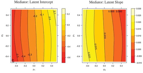
We present two sets of graphs to visually summarize varying degrees of confounding effects on the point and interval estimates for each indirect effect: sensitivity contour plot and sensitivity confidence band plot. The sensitivity contour plots, shown in Figure 5, display the magnitude of the indirect effect as a function of the confounder correlations. For example, panel-a in Figure 5 shows the contour plot for the indirect effect estimate through the mediator latent intercept. The x-axis and y-axis represent the range of values for the confounder correlations between the latent intercept and Y (${\rho }_1$) and latent slope and Y (${\rho }_2$), respectively. Each contour line illustrates all the combinations of the values for the two confounder correlations that result in the same indirect effect estimate. A value for the indirect effect corresponding to each contour line is displayed adjacent to the line. For the indirect effect through the intercept, the estimates range roughly from −0.5 to −0.1 for ρ₁ ≤ .2 and ρ₂ ≤ .5. Given the original estimate for the indirect effect is B (SE) = −0.227 (0.073), 97.5% CI [−0.398, −0.067], the point estimate of the adjusted indirect effect does not appear to change dramatically for the range of confounder correlations. However, as ρ₂ > .2, the sign of the indirect effect estimates changes. For indirect effect estimate through the slope, panel-b in Figure 5 shows that indirect effect estimate roughly ranges from −0.005 to 0.025 for -.5 ≤ ρ₁ and ρ₂ ≤ .5. Given the original estimate of the indirect effect is B (SE) = 0.01 (0.094), 97.5% CI [−0.206, 0.227], the indirect effect estimate did not fall outside of the original CI. In sum, it appears that the values of confounder correlations have considerable impact on the indirect effect through intercept in that sign of the indirect effect changes; on the other hand, the values of confounder correlation appear to have a minimal impact on the indirect effect through slope.

Figure 5 Sensitivity contour plots for the indirect effects. Numbers adjacent to each contour line indicate indirect effect estimates. For the graph on the right, the independent variable, the mediator, and outcome variables are intervention, latent intercept, and heavy drinking as shown in Figure 4. For the graph on the left, the independent variable, the mediator, and outcome variables are intervention, latent slope, and drinking outcome. The confounder parameter ρ₁ is the correlation between the residuals associated with the latent intercept and outcome variable and the confounder parameter ρ₂ is the correlation between the residuals associated with latent slope and the outcome variable.

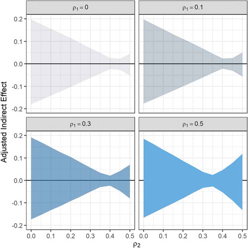
A second way to summarize the effect of omitted confounders is to present sensitivity confidence band plots to examine changes in the CIs. This is advantageous because one can examine the effect of the omitted confounders on the uncertainty about the indirect effects as well as the point estimate. Because there are many combinations of the confounder correlation we use the information from sensitivity contour plots to focus on the range of the confounder correlation values for which the inference about the indirect effect changes. That is, we look at the ranges where the status of a CI containing zero changes to not containing zero and vice versa. Figure 6 shows four panels of 97.5% confidence bands for the indirect effect through intercept; each panel corresponds to a fixed value of ρ₂ where the x-axis shows a more restricted range of values, 0 ≤ ρ₁ ≤ .5, and y-axis shows indirect effect values. We chose positive values for ρ₂ because the results were identical to the corresponding negative values. For example, the confidence band plots were identical for ρ₂ = ± .1. Of course, one may choose different positive or negative values for ρ₂ in a different context. As the value of ρ₂ increases from small (.1) to medium (.3) and then to large (.5), the regions of non-significance corresponding to ρ₁ were roughly (.35, .40), (.30, .42), and (.25, .37), respectively. Below the lower limit of ρ₁ for each non-significance region, the CIs contain negative indirect effect estimates while above the upper limit of ρ₁ for the non-significance region, the CIs contain the positive indirect effect estimates. Figure 7 illustrates the panel plots of confidence bands for the indirect effect estimate through the slope for four values of ρ₁. The x-axis shows the values for ρ₂ between 0 and .5. In each panel, as ρ₂ becomes larger the confidence band becomes narrower and then widens. For all values of ρ₂, however, all the confidence bands contain zero. This shows the inference about the indirect effect through the slope is robust in that the CIs contain zero as the confounder correlation ρ₂ increases from zero to large.

Figure 6 Sensitivity confidence band graphs of 97.5% CIs for indirect effect through the mediator latent intercept. The x-axis on each panel graph shows the confounder parameter ρ₁, which is the correlation between the residuals associated with the latent intercept and outcome variable for the correlated augmented model in Figure 4. The confounder parameter, ρ₂, on top of each panel graph is the correlation between the residuals associated with latent slope and the outcome variable in Figure 4. The y-axis shows indirect effect estimate as a function of the confounder correlation parameters. The ribbon in each graph shows the 97.5% CI bands.

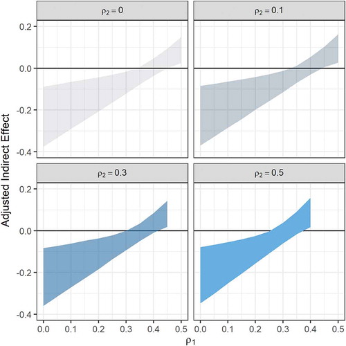
Figure 7 Sensitivity confidence band graphs of 97.5% CIs for the indirect effect through the mediator latent slope. The x-axis on each panel graph shows the confounder parameter ρ₂, which is the correlation between the residuals associated with the latent slope and outcome variable for the correlated augmented model in Figure 4. The confounder parameter, ρ₁, on top of each panel graph is the correlation between the residuals associated with latent intercept and the outcome variable in Figure 4. The y-axis shows indirect effect estimate as a function of the confounder correlation parameters. The ribbon in each graph shows the 97.5% CI bands.

CONCLUSION AND SUMMARY

LGCMMs have become more common in applied contexts to study whether some treatment variable is expected to affect an outcome via changes in some mediating process. Given the growing popularity of this model in the field (see Hallgren et al., 2018), it is critically important to check underlying assumptions to ensure valid results. One of these assumptions is an untestable assumption that there are not omitted confounders from the model. For LGCMM, the no omitted confounder assumption implies that there should be no omitted variable that influences the two mediators as well as the outcome variable. Furthermore, there should be no omitted variable that is influenced by the independent variable X that in turn would influence the mediator and outcome variables.

The current study provides an extension of other recent work (e.g., Bind et al., 2016; Harring et al., 2017; Imai, Keele, & Tingley, 2010; Tofighi & Kelley, 2016), by developing and testing a method for sensitivity analysis in LGCMM. We proposed a technique termed CAMSA for models with two mediators, with an application to LGCMM. CAMSA uses a correlated augmented model to represent cumulative and linear effects of one or more potential confounders. We presented analytic results showing that the confounder covariances between residuals associated with the mediators (latent intercept and slope) and the outcome variable account for confounding effects. We presented formulas to compute the model parameters from the confounder correlations (sensitivity parameters) as the correlation values are more convenient to quantify confounding bias. For multiple combinations of the values for the confounder correlations, CAMSA estimates the correlated augmented model and generates point and interval estimates for the indirect effects, iteratively.

One advantage of the correlated augmented model is using confounder correlations (sensitivity parameters) to quantify confounder bias. Using confounder correlation is more convenient in that one can directly quantify the confounder effects in terms of confounder correlations given analytic formulas. In addition, the correlated augmented model is suitable for mediation models where the endogenous variables are latent. A second advantage of CAMSA is that it can be implemented within the SEM framework and estimated using available software, such as Mplus (L. K. Muthén & Muthén, 2017). We provided an application of CAMSA using an empirical example. An R (R Development Core Team., 2017) script to conduct sensitivity analysis using Mplus along with the instruction on how to use R and Mplus to conduct sensitivity analysis is provided in the Supplemental Materials.

Another noteworthy aspect of conducting sensitivity analysis is the summary and interpretation of point and interval estimates as a function of many combinations of the confounder correlation values. We presented sensitivity contour plots that visually illustrate point estimates of the two indirect effects as a function of confounder correlations, as well as a second visual summary of the results that is the sensitivity confidence band plot. For each indirect effect, the sensitivity confidence band plot illustrates the effect of confounder bias on the confidence intervals of the indirect effect estimates. We recommend researchers try several ranges of the values for both confounder correlations shown on the x-axis and the panel to capture important features of the effects confounding on the interval estimates for an indirect effect.

As mentioned previously, the no-omitted confounder assumption is one of the several specification assumptions underlying a mediation model. Additional assumptions include correct functional form of the relationships between the variables, correct distributional assumptions of the residuals, no outliers, no non-random missing data due to attrition, and no measurement error (Baraldi & Enders, 2010; Fritz, Kenny, & MacKinnon, 2016; Fritz & MacKinnon, 2007; James & Brett, 1984; Judd & Kenny, 1981; MacKinnon, 2008). In addition, within the SEM framework, there are additional statistical distributional assumptions and sample size requirements that need to be satisfied when SEM is used to estimate a mediation model (Hoyle, 2012; Kline, 2016; West, Finch, & Curran, 1995). One must be prudent in examining the combined effect of violation of one or more of these assumptions along with violation of the no omitted confounder assumption. For example, a study showed that combined measurement error and omitted confounder effect can have either a heightened or mitigated combined biasing effect on the indirect effect (Fritz et al., 2016). It is recommended that one would account for the effect of the measurement error by using latent variables.

We also note CAMSA is not suitable for a mediation model with observed endogenous variables because the model would not be identified even though correlations between the residuals are fixed (B. Muthén & Asparouhov, 2015). For such models, we recommend one conduct sensitivity analysis using the latent (phantom variable) augmented model (Harring et al., 2017; Tofighi & Kelley, 2016). It is also possible to extend CAMSA to mediation models with three or more covarying as well as sequential related latent mediators. However, the extension requires additional consideration about confounder correlations and analytic derivation to model confounding effects on all the mediators and outcome variable. The extension remains a topic of future study. Much prior research on sensitivity analysis has focused on the randomized case. With nonrandomized X, there are confounders of the X to M relation. Consequently, equations for calculating sensitivity to confounding would be applied to the X and M relation, and then these equations would need to be developed to include sensitivity to confounding of both the X to M and M to Y relations. The analytical techniques in this paper could be extended to this case and represent a topic for future development. One should be prudent in interpreting the results of the sensitivity analysis. Statistical sensitivity analysis results should be further justified by the researcher as to why the conclusion is consistent with substantive theory and previous research. When the results about the significance of the indirect effects change qualitatively based on values of confounder correlations then a researcher might need to further probe the model and its underlying theory, design of the study, and implementation of the proposed study, as well as check for additional statistical specification assumptions of the mediation model (MacKinnon, 2008; MacKinnon, Fairchild, & Fritz, 2007; MacKinnon & Pirlott, 2015; Preacher, 2015).

Additional information

Funding

This work was supported by NIAAA R01 [grant number AA025539 to Katie Witkiewitz and Davood Tofighi: MPIs] and NIDA [grant number R37DA09757 to (David P. MacKinnon: PI].

Notes

¹ Like latent growth curve model, linear mixed (multilevel) model is used to analyze multilevel data (Raudenbush & Bryk, 2002; Snijders & Bosker, 2011). For similarities and differences between the two techniques, refer to Curran (2003) and Willett and Bub (2005).

² Correlating residuals as a place holder to model an effect has been suggested in SEM literature. For example, Cole, Ciesla, and Steiger (2007) argue for using correlated residuals in a latent variable model to estimate common method (common method variance) effect. We used the same concept to account for the omitted confounder effect in CAMSA except that we fix the confounder covariances between the residuals to specific values.

Appendix

Analytic results for the latent augmented model

In deriving the above expression, we use the following relations.

a) $cov\left(\varpi ,x_i\right)=0$ because $x_i$ is randomized, it neither influences nor is influenced by ϖ. That is, we assume ϖ and $x_i$ to be orthogonal (independent)

b) $cov\left(\varpi ,{\zeta }_{0i}^{\ast }\right)=cov\left(\varpi ,{\zeta }_{1i}^{\ast }\right)=0\mathrm{a}\mathrm{n}\mathrm{d}cov\left(\varpi ,{\zeta }_{0i}^{\ast }|x\right)=cov\left(\varpi ,{\zeta }_{1i}^{\ast }|x\right)=0$ . These expressions hold because we assume that ϖ models all the omitted confounders that influence ${\eta }_0$ and ${\eta }_1$ , and ϖ and $x_i$ are independent.

c) $cov\left(x_i,{\zeta }_{0i}^{\ast }\right)=cov\left(x_i,{\zeta }_{1i}^{\ast }\right)=0$ and $cov\left(x_i,{\zeta }_{0i}^{\ast }|\varpi \right)=cov\left(x_i,{\zeta }_{1i}^{\ast }|\varpi \right)=0$ . These expressions hold because we assume that ϖ models all the omitted confounders that influence ${\eta }_0$ and ${\eta }_1$ , and ϖ and $x_i$ are independent.

d) We also assume constant variance: $var\left({\zeta }_{0i}^{\ast }|x_i,\varpi \right)={\sigma }_{{\zeta }_0{,}^{\ast }}^2$ $var\left({\zeta }_{1i}^{\ast }|x_i,\varpi \right)={\sigma }_{{\zeta }_1^{\ast }}^2$ , and $var\left({\epsilon }_i^{\ast }|x_i,\varpi ,\hspace{0.17em}{\eta }_{i0},{\eta }_{10}\right)={\sigma }_{{\epsilon }^{\ast }}^2$ .

Now, we derive the following expressions. The expression for $\mathrm{c}\mathrm{o}\mathrm{v}\left({\eta }_{i0},{\eta }_{i1}|x\right)$ in Equation (5) is derived as follows:

$\mathrm{c}\mathrm{o}\mathrm{v}\left({\eta }_{i0},{\eta }_{i1}|x\right)=cov({\alpha }_0^{\ast }+{\gamma }_{01}^{\ast }{x}_i+{\gamma }_{02}^{\ast }\varpi +{\zeta }_{0i}^{\ast },{\alpha }_1^{\ast }+{\gamma }_{11}^{\ast }{x}_i+{\gamma }_{12}^{\ast }\varpi +{\zeta }_{1i}^{\ast }|x)=cov({\gamma }_{02}^{\ast }\varpi +{\zeta }_{0i}^{\ast },{\gamma }_{12}^{\ast }\varpi +{\zeta }_{1i}^{\ast }|x)={\sigma }_{\varpi }^2{\gamma }_{02}^{\ast }{\gamma }_{12}^{\ast }+{\sigma }_{{\zeta }_0^{\ast },{\zeta }_1^{\ast }}$

The expressions in and are obtained as follows:

(A1) ${\sigma }_{{\eta }_0,\varpi |x}=\mathrm{c}\mathrm{o}\mathrm{v}({\alpha }_0^{\ast }+{\gamma }_{01}^{\ast }{x}_i+{\gamma }_{02}^{\ast }\varpi +{\zeta }_{0i}^{\ast },\varpi |x)=\mathrm{c}\mathrm{o}\mathrm{v}({\gamma }_{02}^{\ast }\varpi +{\zeta }_{0i}^{\ast },\varpi |x)={\gamma }_{02}^{\ast }{\sigma }_{\varpi }^2$(A1)

(A2) ${\sigma }_{{\eta }_1,\varpi |x}=cov\left({\eta }_1,\varpi |x\right)=\mathrm{c}\mathrm{o}\mathrm{v}({\alpha }_1^{\ast }+{\gamma }_{11}^{\ast }{x}_i+{\gamma }_{12}^{\ast }\varpi +{\zeta }_{1i}^{\ast },\varpi |x)=cov\left({\gamma }_{12}^{\ast }\varpi +{\zeta }_{1i}^{\ast },\varpi |x\right)={\gamma }_{12}^{\ast }{\sigma }_{\varpi }^2$(A2)

To derive the expressions in Equations (9)–(11), we first need to obtain expressions for ${\sigma }_{{\eta }_0,\varpi |x}$ and ${\sigma }_{{\eta }_1,\varpi |x}$, given in Equations (A1) and (A2), ${\sigma }_{{\eta }_0,\varpi }$, ${\sigma }_{{\eta }_1,\varpi }{\sigma }_{{\eta }_0}^2$, ${\sigma }_{{\eta }_0|x}^2$ , ${\sigma }_{{\eta }_1}^2$ , ${\sigma }_{{\eta }_1|x}^2$ , ${\rho }_{{\eta }_0,\varpi }$ , ${\rho }_{{\eta }_0,\varpi |x}$ , ${\rho }_{{\eta }_1,\varpi }$ , ${\rho }_{{\eta }_1,\varpi |x}$ , ${\sigma }_{y,\varpi }$ and ${\rho }_{y,\varpi }$ . We first obtain the conditional and unconditional variance of the growth factors. Given Equation (2), the unconditional variance of the latent intercept is as follows:

(A3) $\begin{array}{rl}& {\sigma }_{{\eta }_0}^2=var\left({\alpha }_0^{\ast }+{\gamma }_{01}^{\ast }{x}_i+{\gamma }_{02}^{\ast }\varpi +{\zeta }_{0i}^{\ast }\right)\\ & ={\left({\gamma }_{01}^{\ast }\right)}^2{\sigma }_x^2+{\left({\gamma }_{02}^{\ast }\right)}^2{\sigma }_{\varpi }^2+{\sigma }_{{\zeta }_0^{\ast }}^2+{\gamma }_{01}^{\ast }{\gamma }_{02}^{\ast }\mathrm{c}\mathrm{o}\mathrm{v}\left(x_i,\varpi \right)\\ & +{\gamma }_{01}^{\ast }cov\left(x_i,{\zeta }_{0i}^{\ast }\right)+{\gamma }_{02}^{\ast }\mathrm{c}\mathrm{o}\mathrm{v}\left(\varpi ,{\zeta }_{0i}^{\ast }\right)\\ & ={\left({\gamma }_{01}^{\ast }\right)}^2{\sigma }_x^2+{\left({\gamma }_{02}^{\ast }\right)}^2{\sigma }_{\varpi }^2+{\sigma }_{{\zeta }_0^{\ast }}^2\end{array}$(A3)

The conditional variance of the latent intercept is as follows:

(A4) ${\sigma }_{{\eta }_0|x}^2=var\left({\alpha }_0^{\ast }+{\gamma }_{01}^{\ast }{x}_i+{\gamma }_{02}^{\ast }\varpi +{\zeta }_{0i}^{\ast }|x\right)=var\left({\gamma }_{02}^{\ast }\varpi +{\zeta }_{0i}^{\ast }|x\right)={\left({\gamma }_{02}^{\ast }\right)}^2{\sigma }_{\varpi }^2+{\sigma }_{{\zeta }_0^{\ast }}^2$(A4)

Given Equation (3), the unconditional variance of the latent slope is as follows:

(A5) $\begin{array}{c}{\sigma }_{{\eta }_1}^2=var\left({\alpha }_1^{\ast }+{\gamma }_{11}^{\ast }{x}_i+{\gamma }_{12}^{\ast }\varpi +{\zeta }_{1i}^{\ast }\right)\\ ={\left({\gamma }_{11}^{\ast }\right)}^2{\sigma }_x^2+{\sigma }_{\varpi }^2{\left({\gamma }_{12}^{\ast }\right)}^2+{\sigma }_{{\zeta }_1^{\ast }}^2+{\gamma }_{11}^{\ast }{\gamma }_{12}^{\ast }cov\left(x_i,\varpi \right)\\ +{\gamma }_{11}^{\ast }cov\left(x_i,{\zeta }_{1i}^{\ast }\right)+{\gamma }_{12}^{\ast }cov\left(\varpi ,{\zeta }_{1i}^{\ast }\right)\\ ={\left({\gamma }_{11}^{\ast }\right)}^2{\sigma }_x^2+{\left({\gamma }_{12}^{\ast }\right)}^2{\sigma }_{\varpi }^2+{\sigma }_{{\zeta }_1^{\ast }}^2\end{array}$(A5)

The conditional variance of latent slope is as follows:

(A6) ${\sigma }_{{\eta }_1|x}^2=var\left({\alpha }_1^{\ast }+{\gamma }_{11}^{\ast }{x}_i+{\gamma }_{12}^{\ast }\varpi +{\zeta }_{1i}^{\ast }|x_i\right)={\left({\gamma }_{12}^{\ast }\right)}^{2}var\left(\varpi |x_i\right)+var\left({\zeta }_{1i}^{\ast }|x_i\right)={\left({\gamma }_{12}^{\ast }\right)}^2{\sigma }_{\varpi }^2+{\sigma }_{{\zeta }_1^{\ast }}^2$(A6)

Next, we compute the unconditional covariance between the latent growth factors and ϖ.

(A7) ${\sigma }_{{\eta }_0,\varpi }=cov\left({\alpha }_0^{\ast }+{\gamma }_{01}^{\ast }{x}_i+{\gamma }_{02}^{\ast }\varpi +{\zeta }_{0i}^{\ast },\varpi \right)={\gamma }_{01}^{\ast }cov\left(x_i,\varpi \right)+{\gamma }_{02}^{\ast }{\sigma }_{\varpi }^2+cov\left({\zeta }_{0i}^{\ast },\varpi \right)={\gamma }_{02}^{\ast }{\sigma }_{\varpi }^2$(A7)

(A8) ${\sigma }_{{\eta }_1,\varpi }=cov\left({\alpha }_1^{\ast }+{\gamma }_{11}^{\ast }{x}_i+{\gamma }_{12}^{\ast }\varpi +{\zeta }_{1i}^{\ast },\varpi \right)={\gamma }_{11}^{\ast }cov\left(x_i,\varpi \right)+{\gamma }_{12}^{\ast }{\sigma }_{\varpi }^2+cov\left({\zeta }_{1i}^{\ast },\varpi \right)={\gamma }_{12}^{\ast }{\sigma }_{\varpi }^2$(A8)

Next, we compute the conditional and unconditional correlation between the latent growth factors and ϖ. Given Equations (A3) and (A7), the unconditional correlation between the latent intercept and ϖ is as follows:

(A9) ${\rho }_{{\eta }_0,\varpi }=\frac{{\sigma }_{{\eta }_0,\varpi }}{{\sigma }_{{\eta }_0}{\sigma }_{\varpi }}=\frac{{\gamma }_{02}^{\ast }{\sigma }_{\varpi }}{\sqrt{{\left({\gamma }_{01}^{\ast }\right)}^2{\sigma }_x^2+{\sigma }_{\varpi }^2{\left({\gamma }_{02}^{\ast }\right)}^2+{\sigma }_{{\zeta }_0^{\ast }}^2}}=\frac{{\gamma }_{02}^{\ast }{\sigma }_{\varpi }}{{\sigma }_{{\eta }_0}}$(A9)

Given Equations (A1) and (A4), the conditional correlation between the latent intercept and ϖ is as follows:

${\rho }_{{\eta }_0,\varpi |x}=\frac{{\sigma }_{{\eta }_0,\varpi |x}}{{\sigma }_{{\eta }_0|x}{\sigma }_{\varpi }}=\frac{{\gamma }_{02}^{\ast }{\sigma }_{\varpi }}{\sqrt{{\sigma }_{\varpi }^2{\left({\gamma }_{02}^{\ast }\right)}^2+{\sigma }_{{\zeta }_0^{\ast }}^2}}=\frac{{\gamma }_{02}^{\ast }{\sigma }_{\varpi }}{{\sigma }_{{\eta }_0|x}}$

Given Equations (A5) and (A8), the unconditional correlation between the latent slope and ϖ is as follows:

(A10) ${\rho }_{{\eta }_1,\varpi }=\frac{{\sigma }_{{\eta }_1,\varpi }}{{\sigma }_{{\eta }_1}{\sigma }_{\varpi }}=\frac{{\gamma }_{12}^{\ast }{\sigma }_{\varpi }}{\sqrt{{\left({\gamma }_{11}^{\ast }\right)}^2{\sigma }_x^2+{\sigma }_{\varpi }^2{\left({\gamma }_{12}^{\ast }\right)}^2+{\sigma }_{{\zeta }_1^{\ast }}^2}}=\frac{{\gamma }_{12}^{\ast }{\sigma }_{\varpi }}{{\sigma }_{{\eta }_1}}$(A10)

Given Equations (A2) and (A6), the conditional correlation between the latent slope and ϖ is as follows:

${\rho }_{{\eta }_1,\varpi |x}=\frac{{\sigma }_{{\eta }_1,\varpi |x}}{{\sigma }_{{\eta }_1|x}{\sigma }_{\varpi }}=\frac{{\gamma }_{12}^{\ast }{\sigma }_{\varpi }}{\sqrt{{\sigma }_{\varpi }^2{\left({\gamma }_{12}^{\ast }\right)}^2+{\sigma }_{{\zeta }_1^{\ast }}^2}}=\frac{{\gamma }_{12}^{\ast }{\sigma }_{\varpi }}{{\sigma }_{{\eta }_1|x}}$

Next, we derive ${\sigma }_{y,\varpi }$ and ${\rho }_{y,\varpi }$ .

${\sigma }_{y,\varpi }=cov\left({\nu }^{\ast }+{\kappa }^{\ast }{x}_i+{\lambda }_1^{\ast }{\eta }_{i0}+{\lambda }_2^{\ast }{\eta }_{i1}+{\lambda }_3^{\ast }\varpi +{\epsilon }_i^{\ast },\varpi \right)={\lambda }_1^{\ast }cov\left({\eta }_{i0},\varpi \right)+{\lambda }_2^{\ast }cov\left({\eta }_{i1},\varpi \right)+{\lambda }_3^{\ast }{\sigma }_{\varpi }^2=\left({\lambda }_1^{\ast }{\gamma }_{02}^{\ast }+{\lambda }_2^{\ast }{\gamma }_{12}^{\ast }+{\lambda }_3^{\ast }\right){\sigma }_{\varpi }^2$

(A11) ${\rho }_{y,\varpi }=\frac{{\sigma }_{y_i,\varpi }}{{\sigma }_y{\sigma }_{\varpi }}=\frac{{\sigma }_{\varpi }}{{\sigma }_y}\left({\lambda }_1^{\ast }{\gamma }_{02}^{\ast }+{\lambda }_2^{\ast }{\gamma }_{12}^{\ast }+{\lambda }_3^{\ast }\right)$(A11)

Finally, isolating ${\gamma }_{02}^{\ast }$ in Equation (A9), we arrive at the expression in Equation (9). Isolating ${\gamma }_{12}^{\ast }$ in Equation (A10), we arrive at the expression in Equation (10). Isolating ${\lambda }_3^{\ast }$ in Equation (A11) would result in Equation (11).

In addition, we compute the expected valued for the latent growth factors and $y_i$ . We use the expected values to compare the respective residuals with the ones from the correlated augmented model in the next section:

(A12) $\mathrm{E}\left({\eta }_{0i}|x_i\right)=\mathrm{E}\left[\mathrm{E}\left({\eta }_{0i}|x_i,\varpi \right)\right]=\mathrm{E}\left[\mathrm{E}\left({\alpha }_0^{\ast }+{\gamma }_{01}^{\ast }{x}_i+{\gamma }_{02}^{\ast }\varpi +{\zeta }_{0i}^{\ast }|x_i,\varpi \right)\right]={\alpha }_0^{\ast }+{\gamma }_{01}^{\ast }{x}_i+\mathrm{E}\left[{\gamma }_{02}^{\ast }\varpi +\mathrm{E}\left({\zeta }_{0i}^{\ast }|x_i,\varpi \right)\right]={\alpha }_0^{\ast }+{\gamma }_{01}^{\ast }{x}_i$(A12)

(A13) $\mathrm{E}\left({\eta }_{1i}|x_i\right)=\mathrm{E}\left[\mathrm{E}\left({\eta }_{1i}|x_i,\varpi \right)\right]=\mathrm{E}\left[\mathrm{E}\left({\alpha }_1^{\ast }+{\gamma }_{11}^{\ast }{x}_i+{\gamma }_{12}^{\ast }\varpi +{\zeta }_{1i}^{\ast }|x_i,\varpi \right)\right]={\alpha }_1^{\ast }+{\gamma }_{11}^{\ast }{x}_i+\mathrm{E}\left[{\gamma }_{12}^{\ast }\varpi +\mathrm{E}\left({\zeta }_{1i}^{\ast }|x_i,\varpi \right)\right]={\alpha }_1^{\ast }+{\gamma }_{11}^{\ast }{x}_i$(A13)

(A14) $\mathrm{E}\left(y_i|x_i\right)=\mathrm{E}\left({\nu }^{\ast }+{\kappa }^{\ast }{x}_i+{\lambda }_1^{\ast }{\eta }_{i0}+{\lambda }_2^{\ast }{\eta }_{i1}+{\lambda }_3^{\ast }\varpi +{\epsilon }_i^{\ast }|x_i,{\eta }_{0i},{\eta }_{1i}\right)={\nu }^{\ast }+{\kappa }^{\ast }{x}_i+{\lambda }_1^{\ast }{\eta }_{i0}+{\lambda }_2^{\ast }{\eta }_{i1}$(A14)

Correlated augmented model

First, we derive the mean and variance of the mediators (growth factors) for the correlated augmented model and then compare them with the corresponding expected values from the latent augmented model. To show equivalency, the parameters from the correlated augmented model must be a function of the corresponding parameters from the latent augmented model:

(A15) $\begin{array}{c}\mathrm{E}\left({\eta }_{0i}|x_i\right)=\mathrm{E}\left[\mathrm{E}\left({\eta }_{0i}|x_i,\varpi \right)\right]=\mathrm{E}\left[\mathrm{E}\left({\alpha }_0^{\ast \ast }+{\gamma }_{01}^{\ast \ast }{x}_i+{\zeta }_{0i}^{\ast \ast }|x_i,\varpi \right)\right]={\alpha }_0^{\ast \ast }\\ +{\gamma }_{01}^{\ast \ast }{x}_i+\mathrm{E}\left[\mathrm{E}\left({\zeta }_{0i}^{\ast \ast }|x_i,\varpi \right)\right]={\alpha }_0^{\ast \ast }+{\gamma }_{01}^{\ast \ast }{x}_i+\mathrm{E}({\zeta }_{0i}^{\ast \ast }|\varpi )\\ ={\alpha }_0^{\ast \ast }+{\gamma }_{01}^{\ast \ast }{x}_i\end{array}$(A15)

(A16) $\mathrm{E}\left({\eta }_{1i}|x_i\right)=\mathrm{E}\left[\mathrm{E}\left({\eta }_{1i}|x_i,\varpi \right)\right]=\mathrm{E}\left[\mathrm{E}\left({\alpha }_1^{\ast \ast }+{\gamma }_{11}^{\ast \ast }{x}_i+{\zeta }_{1i}^{\ast \ast }|x_i,\varpi \right)\right]={\alpha }_1^{\ast \ast }+{\gamma }_{11}^{\ast \ast }{x}_i+\mathrm{E}\left[\mathrm{E}\left({\zeta }_{1i}^{\ast \ast }|x_i,\varpi \right)\right]={\alpha }_1^{\ast \ast }+{\gamma }_{11}^{\ast \ast }{x}_i$(A16)

(A17) $\mathrm{E}\left(y_i|x_i\right)=\mathrm{E}\left({\nu }^{\ast \ast }+{\kappa }^{\ast \ast }{x}_i+{\lambda }_1^{\ast \ast }{\eta }_{0i}+{\lambda }_2^{\ast \ast }{\eta }_{1i}+{\epsilon }_y^{\ast \ast }|x_i,{\eta }_{0i},{\eta }_{1i}\right)={\nu }^{\ast \ast }+{\kappa }^{\ast \ast }{x}_i+{\lambda }_1^{\ast \ast }{\eta }_{0i}+{\lambda }_2^{\ast \ast }{\eta }_{1i}$(A17)

Comparing the expected values of the correlated augmented model with the corresponding expected values from the latent augmented model, one can see that there is a one-to-one relationship between the two model parameters. Furthermore, we can use the expected values to isolate the residuals for latent growth factors and $y_i$ in each model. Then, comparing the corresponding residuals from the two models, the following holds:

${\zeta }_{0i}^{\ast \ast }={\gamma }_{02}^{\ast }\varpi +{\zeta }_{0i}^{\ast }$

${\zeta }_{1i}^{\ast \ast }={\gamma }_{12}^{\ast }\varpi +{\zeta }_{1i}^{\ast }$

${\epsilon }_i^{\ast \ast }={\lambda }_3^{\ast }\varpi +{\epsilon }_i^{\ast }$

We use the relationships between the residuals to compute the covariance and ultimately correlation between residuals in the correlated augmented model shown in Equations (16)–(19) in terms of the parameters from the latent augmented model:

${\sigma }_{{\epsilon }_y^{\ast \ast },{\zeta }_0^{\ast \ast }}=\mathrm{c}\mathrm{o}\mathrm{v}\left({\epsilon }_i^{\ast \ast },{\zeta }_0^{\ast \ast }\right)=cov({\epsilon }_i^{\ast \ast },{\zeta }_0^{\ast \ast }|{\eta }_{i0},{\eta }_{10},x)=cov\left({\lambda }_3^{\ast }\varpi +{\epsilon }_i^{\ast },{\gamma }_{02}^{\ast }\varpi +{\zeta }_{0i}^{\ast }\right)={\gamma }_{02}^{\ast }{\lambda }_3^{\ast }{\sigma }_{\varpi }^2$

${\sigma }_{{\epsilon }_y^{\ast \ast },{\zeta }_1^{\ast \ast }}=cov\left({\epsilon }_i^{\ast \ast },{\zeta }_1^{\ast \ast }\right)=cov({\epsilon }_i^{\ast \ast },{\zeta }_1^{\ast \ast }|{\eta }_{i0},{\eta }_{10},x)=cov\left({\lambda }_3^{\ast }\varpi +{\epsilon }_i^{\ast },{\gamma }_{12}^{\ast }\varpi +{\zeta }_{1i}^{\ast }\right)={\gamma }_{12}^{\ast }{\lambda }_3^{\ast }{\sigma }_{\varpi }^2$

Next, we derive the following variances:

${\sigma }_{{\epsilon }_y^{\ast \ast }}^2={\left({\lambda }_3^{\ast }\right)}^2{\sigma }_{\varpi }^2+{\sigma }_{{\epsilon }_y^{\ast }}^2$

${\sigma }_{{\zeta }_0^{\ast \ast }}^2={\left({\gamma }_{02}^{\ast }\right)}^2{\sigma }_{\varpi }^2+{\sigma }_{{\zeta }_0^{\ast }}^2$

${\sigma }_{{\zeta }_1^{\ast \ast }}^2={\left({\gamma }_{12}^{\ast }\right)}^2{\sigma }_{\varpi }^2+{\sigma }_{{\zeta }_1^{\ast }}^2$

Finally, the derive the following correlations shown in Equations (18) and (19):

${\rho }_{{\epsilon }_y^{\ast \ast },{\zeta }_0^{\ast \ast }}=\frac{{\sigma }_{{\epsilon }_y^{\ast \ast },{\zeta }_0^{\ast \ast }}}{{\sigma }_{{\epsilon }_y^{\ast \ast }}{\sigma }_{{\zeta }_0^{\ast \ast }}}=\frac{{\gamma }_{02}^{\ast }{\lambda }_3^{\ast }\hspace{0.17em}{\sigma }_{\varpi }^2}{\sqrt{{\left({\lambda }_3^{\ast }\right)}^2{\sigma }_{\varpi }^2+{\sigma }_{{\epsilon }_y^{\ast }}^2}\sqrt{{\left({\gamma }_{02}^{\ast }\right)}^2{\sigma }_{\varpi }^2+{\sigma }_{{\zeta }_0^{\ast }}^2}}$

${\rho }_{{\epsilon }_y^{\ast \ast },{\zeta }_1^{\ast \ast }}=\frac{{\sigma }_{{\epsilon }_y^{\ast \ast },{\zeta }_1^{\ast \ast }}}{{\sigma }_{{\epsilon }_y^{\ast \ast }}{\sigma }_{{\zeta }_1^{\ast \ast }}}=\frac{{\gamma }_{12}^{\ast }{\lambda }_3^{\ast }{\sigma }_{\varpi }^2}{\sqrt{{\left({\lambda }_3^{\ast }\right)}^2{\sigma }_{\varpi }^2+{\sigma }_{{\epsilon }_y^{\ast }}^2}\sqrt{{\left({\gamma }_{12}^{\ast }\right)}^2{\sigma }_{\varpi }^2+{\sigma }_{{\zeta }_1^{\ast }}^2}}$

Below we derive the relationships between the covariance between residuals of the growth factors in the correlated augmented model and the corresponding covariance in the latent augmented model.

${\sigma }_{{\zeta }_1^{\ast \ast },{\zeta }_0^{\ast \ast }}=cov({\zeta }_1^{\ast \ast },{\zeta }_0^{\ast \ast }|{\eta }_{i0},{\eta }_{10},x)=cov\left({\gamma }_{12}^{\ast }\varpi +{\zeta }_{1i}^{\ast },{\gamma }_{02}^{\ast }\varpi +{\zeta }_{0i}^{\ast }\right)={\gamma }_{02}^{\ast }{\gamma }_{12}^{\ast }{\sigma }_{\varpi }^2+{\sigma }_{{\zeta }_0^{\ast },{\zeta }_1^{\ast }}$

This is the expression is shown in Equation (5).

References

- Allison, P. D. (2005). Fixed effects regression methods for longitudinal data using SAS (1st ed.). Cary, NC: SAS Publishing.
- Alvarez, A. N., & Juang, L. P. (2010). Filipino Americans and racism: A multiple mediation model of coping. Journal of Counseling Psychology, 57, 167–178. doi:10.1037/a0019091
- Baraldi, A. N., & Enders, C. K. (2010). An introduction to modern missing data analyses. Journal of School Psychology, 48, 5–37. doi:10.1016/j.jsp.2009.10.001
- Bartholomew, D. J., Knott, M., & Moustaki, I. (2011). Latent variable models and factor analysis: A unified approach (3rd ed.). Chichester, UK: Wiley.
- Bind, M.-A. C., VanderWeele, T. J., Coull, B. A., & Schwartz, J. D. (2016). Causal mediation analysis for longitudinal data with exogenous exposure. Biostatistics, 17, 122–134. doi:10.1093/biostatistics/kxv029
- Chen, F., Bollen, K. A., Paxton, P., Curran, P. J., & Kirby, J. B. (2001). Improper solutions in structural equation models: Causes, consequences, and strategies. Sociological Methods & Research, 29(4), 468-508. doi:10.1177/0049124101029004003
- Chen, Z., & Wang, H. (2017). Abusive supervision and employees’ job performance: A multiple mediation model. Social Behavior and Personality, 45(5), 845–858. doi:10.2224/sbp.5657
- Cohen, J. (1988). Statistical power analysis for the behavioral sciences (2nd ed.). Hillsdale, NJ: Erlbaum.
- Cole, D. A., Ciesla, J. A., & Steiger, J. H. (2007). The insidious effects of failing to include design-driven correlated residuals in latent-variable covariance structure analysis. Psychological Methods, 12, 381–398. doi:10.1037/1082-989X.12.4.381
- Cox, M. G., Kisbu-Sakarya, Y., Miočević, M., & MacKinnon, D. P. (2013). Sensitivity plots for confounder bias in the single mediator model. Evaluation Review, 37, 405–431. doi:10.1177/0193841X14524576
- Curran, P. J. (2003). Have multilevel models been structural equation models all along? Multivariate Behavioral Research, 38, 529–569. doi:10.1207/s15327906mbr3804_5
- Daniel, R. M., De Stavola, B. L., Cousens, S. N., & Vansteelandt, S. (2015). Causal mediation analysis with multiple mediators. Biometrics, 71(1), 1–14. doi:10.1111/biom.12248
- Demiray, B., & Janssen, S. M. J. (2015). The self‐enhancement function of autobiographical memory. Applied Cognitive Psychology, 29, 49–60. doi:10.1002/acp.3074
- Dillon, W. R., Kumar, A., & Mulani, N. (1987). Offending estimates in covariance structure analysis: Comments on the causes of and solutions to Heywood cases. Psychological Bulletin, 101, 126–135. doi:10.1037/0033–2909.101.1.126
- Flannery, B. A., Volpicelli, J. R., & Pettinati, H. M. (1999). Psychometric properties of the Penn Alcohol Craving Scale. Alcoholism: Clinical and Experimental Research, 23(8), 1289–1295. doi:10.1111/acer.1999.23.issue-8
- Fritz, M. S., Kenny, D. A., & MacKinnon, D. P. (2016). The combined effects of measurement error and omitting confounders in the single-mediator model. Multivariate Behavioral Research, 51(5), 681–697. doi:10.1080/00273171.1224154.2016
- Fritz, M. S., & MacKinnon, D. P. (2007). Required sample size to detect the mediated effect. Psychological Science, 18, 233–239. doi:10.1111/j.1467-9280.01882.x.2007
- Grimm, K. J., Ram, N., & Estabrook, R. (2017). Growth modeling: Structural equation and multilevel modeling approaches. New York, NY: Guilford Press.
- Hallgren, K. A., Wilson, A. D., & Witkiewitz, K. (2018). Advancing analytic approaches to address key questions in mechanisms of behavior change research. Journal of Studies on Alcohol and Drugs, 79, 182–189. doi:10.15288/jsad.79.1822018.
- Harring, J. R., McNeish, D. M., & Hancock, G. R. (2017). Using phantom variables in structural equation modeling to assess model sensitivity to external misspecification. Psychological Methods, 22, 616–631. doi:10.1037/met0000103
- Holland, P. W. (1988). Causal Inference, path analysis, and recursive structural equations models. Sociological Methodology, 18, 449–484. doi:10.2307/271055
- Hoyle, R. H. (Ed). (2012). Handbook of structural equation modeling. New York, NY: Guilford Press.
- Imai, K., Keele, L., & Tingley, D. (2010). A general approach to causal mediation analysis. Psychological Methods, 15, 309–334. doi:10.1037/a0020761
- Imai, K., Keele, L., & Yamamoto, T. (2010). Identification, inference and sensitivity analysis for causal mediation effects. Statistical Science, 25, 51–71. doi:10.1214/10-STS321
- Imai, K., & Yamamoto, T. (2013). Identification and sensitivity analysis for multiple causal mechanisms: Revisiting evidence from framing experiments. Political Analysis, 21, 141–171. doi:10.1093/pan/mps040
- James, L. R., & Brett, J. M. (1984). Mediators, moderators, and tests for mediation. Journal of Applied Psychology, 69, 307–321. doi:10.1037/0021–9010.69.2.307
- Judd, C. M., & Kenny, D. A. (1981). Process analysis. Evaluation Review, 5, 602–619. doi:10.1177/0193841X8100500502
- Kenny, D. A. (2004). Correlation and causality. New York, NY: Wiley. Retrieved from http://davidakenny.net/doc/cc_v1.pdf.
- Kenny, D. A., & Milan, S. (2012). Identification: A non-technical discussion of a technical issue. In R. H. Hoyle (Ed.), Handbook of structural equation modeling (pp. 145–163). New York, NY: Guilford Press.
- Kershaw, K. N., Mezuk, B., Abdou, C. M., Rafferty, J. A., & Jackson, J. S. (2010). Socioeconomic position, health behaviors, and C-reactive protein: A moderated-mediation analysis. Health Psychology, 29, 307–316. doi:10.1037/a0019286
- Kline, R. B. (2016). Principles and practice of structural equation modeling (4th ed.). New York, NY: Guilford.
- Kolenikov, S., & Bollen, K. A. (2012). Testing negative error variances: Is a Heywood case a symptom of misspecification?Sociological Methods & Research, 41(1), 124–167. doi:10.1177/0049124112442138
- Kranzler, H. R., Armeli, S., Covault, J., & Tennen, H. (2013). Variation in OPRM1 moderates the effect of desire to drink on subsequent drinking and its attenuation by naltrexone treatment: Naltrexone pharmacogenetics. Addiction Biology, 18, 193–201. doi:10.1111/j.1369-1600.00471.x2012.
- Kreft, I. G. G., De Leeuw, J., & Aiken, L. S. (1995). The effect of different forms of centering in hierarchical linear models. Multivariate Behavioral Research, 30, 1–21. doi:10.1207/s15327906mbr3001_1
- Leung, C.-K., & Lam, K. (1975). A note on the geometric representation of the correlation coefficients. The American Statistician, 29, 128–130. doi:10.2307/2683440
- Ma, Y., Cheng, W., Ribbens, B. A., & Zhou, J. (2013). Linking ethical leadership to employee creativity: Knowledge sharing and self efficacy as mediators. Social Behavior and Personality, 41, 1409–1419. doi:10.2224/sbp.41.9.14092013.
- MacKinnon, D. P. (2008). Introduction to statistical mediation analysis. New York, NY: Erlbaum.
- MacKinnon, D. P., Fairchild, A. J., & Fritz, M. S. (2007). Mediation analysis. Annual Review of Psychology, 58, 593–614. doi:10.1146/annurev085542.psych.58.110405.
- MacKinnon, D. P., & Pirlott, A. G. (2015). Statistical approaches for enhancing causal interpretation of the M to Y relation in mediation analysis. Personality and Social Psychology Review, 19, 30–43. doi:10.1177/1088868314542878
- Mann, K., Roos, C. R., Hoffmann, S., Nakovics, H., Leménager, T., Heinz, A., & Witkiewitz, K. (2018). Precision medicine in alcohol dependence: A controlled trial testing pharmacotherapy response among reward and relief drinking phenotypes. Neuropsychopharmacology, 43, 891–899. doi:10.1038/npp.2822017
- McNeish, D., & Kelley, K. (2018). Fixed effects models versus mixed effects models for clustered data: Reviewing the approaches, disentangling the differences, and making recommendations. Psychological Methods. doi:10.1037/met0000182
- Miller, W. R. (1996). Form 90: A structured assessment interview for drinking and related behaviors. In M. E. Mattson (Ed.), NIAAA Project MATCH Monograph Series (Vol. 5). Bethesda, MD: U.S. Department of Health and Human Services.
- Muthén, B., & Asparouhov, T. (2015). Causal effects in mediation modeling: An introduction with applications to latent variables. Structural Equation Modeling, 22, 12–23. doi:10.1080/10705511.9358432014
- Muthén, L. K., & Muthén, B. O. (2017). Mplus User’s Guide (Version 8). Los Angeles, CA: Muthén & Muthén.
- Pearl, J. (2011). The mediation formula: A guide to the assessment of causal pathways in nonlinear models. In C. Berzuini, P. Dawid, & L. Bernardinell (Eds.), Causality: Statistical Perspectives and Applications (pp. 151–179). Hoboken, NJ: Wiley.
- Pearl, J. (2014). Interpretation and identification of causal mediation. Psychological Methods, 19, 459–481. doi:10.1037/a0036434
- Preacher, K. J. (2015). Advances in mediation analysis: A survey and synthesis of new developments. Annual Review of Psychology, 66, 825–852. doi:10.1146/annurev-psych–010814–015258
- Priesemuth, M., Schminke, M., Ambrose, M. L., & Folger, R. (2014). Abusive supervision climate: A multiple-mediation model of its impact on group outcomes. Academy of Management Journal, 57, 1513–1534. doi:10.5465/amj.2011.0237
- R Development Core Team. (2017). R: A Language and Environment for Statistical Computing (Version 3.4.3). Vienna, Austria: R Foundation for Statistical Computing. Retrieved from http://www.R-project.org/
- Raudenbush, S. W., & Bryk, A. S. (2002). Hierarchical linear models: Applications and data analysis methods (2nd ed.). Thousand Oaks, CA: Sage.
- Rindskopf, D. (1983). Parameterizing inequality constraints on unique variances in linear structural models. Psychometrika, 48(1), 73–83. doi:10.1007/BF02314677
- Rindskopf, D. (1984). Structural equation models: Empirical identification, Heywood cases, and related problems. Sociological Methods & Research, 13, 109–119. doi:10.1177/0049124184013001004.
- Robins, J. M., & Greenland, S. (1992). Identifiability and exchangeability for direct and indirect effects. Epidemiology, 3(2), 143–155. doi:10.1097/00001648-199203000-00013
- Rousseeuw, P. J., & Molenberghs, G. (1994). The shape of correlation matrices. The American Statistician, 48, 276–279. doi:10.2307/2684832.
- Rubin, D. B. (1974). Estimating causal effects of treatments in randomized and nonrandomized studies. Journal of Educational Psychology, 66(5), 688–701. doi:10.1037/h0037350.
- Rubin, D. B. (1978). Bayesian inference for causal effects: The role of randomization. The Annals of Statistics, 6, 34–58. doi:10.1214/aos/1176344064
- Schacht, J. P., Randall, P. K., Latham, P. K., Voronin, K. E., Book, S. W., Myrick, H., & Anton, R. F. (2017). Predictors of naltrexone response in a randomized trial: Reward-related rrain activation, OPRM1 genotype, and smoking status. Neuropsychopharmacology, 42(13), 2640–2653. doi:10.1038/npp74.2017.
- Selig, J. P., & Preacher, K. J. (2009). Mediation models for longitudinal data in developmental research. Research in Human Development, 6, 144–164. doi:10.1080/15427600902911247.
- Singer, J. D., & Willett, J. B. (2003). Applied longitudinal data analysis modeling change and event occurrence. Oxford, MA: Oxford University Press.
- Snijders, T. A. B., & Bosker, R. J. (2011). Multilevel analysis: An introduction to basic and advanced multilevel modeling (2nd ed.). Thousand Oaks, CA: SAGE.
- Strelan, P., Karremans, J. C., & Krieg, J. (2017). What determines forgiveness in close relationships? The role of post‐transgression trust. British Journal of Social Psychology, 56, 161–180. doi:10.1111/bjso.12173
- Talloen, W., Moerkerke, B., Loeys, T., De Naeghel, J., Van Keer, H., & Vansteelandt, S. (2016). Estimation of indirect effects in the presence of unmeasured confounding for the mediator–Outcome relationship in a multilevel 2-1-1 mediation model. Journal of Educational and Behavioral Statistics, 41, 359–391. doi:10.3102/1076998616636855.
- Tofighi, D., & Kelley, K. (2016). Assessing omitted confounder bias in multilevel mediation models. Multivariate Behavioral Research, 51, 86–105. doi:10.1080/00273171.11057362015
- Tofighi, D., & MacKinnon, D. P. (2011). RMediation: An R package for mediation analysis confidence intervals. Behavior Research Methods, 43, 692–700. doi:10.3758/s13428-011-0076–x
- Tofighi, D., West, S. G., & MacKinnon, D. P. (2013). Multilevel mediation analysis: The effects of omitted variables in the 1-1-1 model. British Journal of Mathematical and Statistical Psychology, 66, 290–307. doi:10.1111/j.2044-8317.2012.02051.x
- Valente, M. J., Pelham, W. E. I., Smyth, H., & MacKinnon, D. P. (2017). Confounding in statistical mediation analysis: What it is and how to address it. Journal of Counseling Psychology, 64(6), 659–671. doi:10.1037/cou0000242
- VanderWeele, T. J. (2010). Bias formulas for sensitivity analysis for direct and indirect effects. Epidemiology, 21, 540–551. doi:10.1097/EDE.0b013e3181df191c
- VanderWeele, T. J. (2015). Explanation in causal inference: Methods for mediation and interaction. New York, NY: Oxford University Press.
- Villegas-Gold, R., & Yoo, H. C. (2014). Coping with discrimination among Mexican American college students. Journal of Counseling Psychology, 61(3), 404–413. doi:10.1037/a0036591.
- Von Soest, T., & Hagtvet, K. A. (2011). Mediation analysis in a latent growth curve modeling framework. Structural Equation Modeling: A Multidisciplinary Journal, 18, 289–314. doi:10.1080/10705511.5573442011
- West, S. G., Finch, J. F., & Curran, P. J. (1995). Structural equation models with nonnormal variables: Problems and remedies. In R. H. Hoyle (Ed.), Structural equation modeling: Concepts, issues, and applications (pp. 56–75). Thousand Oaks, CA, US: Sage.
- Willett, J. B., & Bub, K. L. (2005). Structural equation modeling: Latent growth curve analysis. In B. S. Everitt & D. C. Howell (Eds.), Encyclopedia of Statistics in Behavioral Science. Hoboken, NJ: John Wiley & Sons. doi:10.1002/0470013192.bsa599