Latent Class Trees with the Three-Step Approach

Abstract

Latent class (LC) analysis is widely used in the social and behavioral sciences to find meaningful clusters based on a set of categorical variables. To deal with the common problem that a standard LC analysis may yield a large number classes and thus a solution that is difficult to interpret, recently an alternative approach has been proposed, called Latent Class Tree (LCT) analysis. It involves starting with a solution with a small number of “basic” classes, which may subsequently be split into subclasses at the next stages of an analysis. However, in most LC analysis applications, we not only wish to identify the relevant classes, but also want to see how they relate to external variables (covariates or distal outcomes). For this purpose, researchers nowadays prefer using the bias-adjusted three-step method. Here, we show how this bias-adjusted three-step procedure can be applied in the context of LCT modeling. More specifically, an R-package is presented that performs a three-step LCT analysis: it builds a LCT and allows checking how splits are related to the relevant external variables. The new tool is illustrated using a cross-sectional application with multiple indicators on social capital and demographics as external variables and with a longitudinal application with a mood variable measured multiple times during the day and personality traits as external variables.

Keywords:

• Latent classes
• three-step approach
• latent class trees
• mixture models

The goal of any sort of cluster analysis is to determine the number of meaningful subgroups simultaneously with their characteristics. This also applies to Latent Class (LC) modeling, which is a probabilistic clustering tool for categorical variables (Clogg, 1995; Goodman, 1974; Hagenaars, 1990; Lazarsfeld & Henry, 1968; McCutcheon, 1987) in which the classes are interpreted based on their conditional response probabilities (Muthén, 2004).

Typically, researchers estimate LC models with different numbers of classes and select the best model using the likelihood-based statistics, which weigh model fit and complexity (e.g., Akaike information criterion [AIC] or Bayesian information criterion [BIC]). Although, in theory, there is nothing wrong with such a procedure, in practice it is often perceived as being problematic, especially when dealing with large data sets; that is, when the number of variables and/or the number of subjects is large. One problem that occurs in such situations is that the selected number of classes may be rather large. This causes the classes to pick up very specific aspects of the data, which might not be interesting for the research question at hand. Moreover, these specific classes are hard to interpret substantively and compare to each other. A second problem results from the fact that usually one would select a different number of classes depending on the model-selection criterion used. Owing of this, one may wish to inspect multiple solutions, as each of them may reveal specific relevant features in the data. However, it is fully unclear how solutions with different numbers of classes are related, making it very hard to see what a model with $K+1$ classes adds to a model with $K$ classes.

To circumvent the aforementioned issues, van Den Bergh, Schmittmann, and Vermunt (2017) proposed the Latent Class Tree (LCT) modeling approach, which is based on an algorithm for latent-class based density estimation by Van der Palm, van der Ark, and Vermunt (2015). LCT modeling involves imposing a hierarchical tree structure on the latent classes. After deciding on the initial number of “basic” latent classes, the initial classes are treated as parent nodes for which we estimate 1- and 2-class models. If the 2-class model is preferred according to say the BIC, the sample at the parent node is split into “child” nodes and separate data sets are constructed for each of the child nodes with the class membership probabilities serving as weights.¹ Subsequently, each new child node is treated as a parent and it is checked again whether a 2-class model provides a better fit than a 1-class model on the corresponding weighted data set. This procedure continues until no node is split up anymore. This sequential splitting algorithm yields a set of hierarchically connected clusters. The higher-level clusters will typically be the most interesting ones, since these capture the most dominant differences between the individuals in the sample. Lower-level clusters are special cases of higher-level clusters showing certain more specific differences between respondents belonging to the same higher-level cluster. Whether such more specific differences are relevant or not depends on the purpose of the LCT analysis. If this is not the case, one may consider ignoring the lower-level splits concerned.

In most LC analysis applications, the identification of classes is only the first step in an analysis, as researchers are often also interested in how the classes are related to external variables. Two possible approaches for dealing with external variables are the one-step procedure in which these external variables are included in the estimated LC model (Dayton & Macready, 1988; Hagenaars, 1990; Van der HeiHeijden, Dessens, & Bockenholt, 1996; Yamaguchi, 2000) and the three-step procedure in which one makes use of class assignments (Bakk, Oberski, & Vermunt, 2016; Bakk & Vermunt, 2016; Bolck, Croon, & Hagenaars, 2004; Vermunt, 2010). The three-step approach is the more popular one, mainly because researchers find it more practical to separate the construction of the measurement part (in which the number of classes and their relation with the indicator variables are determined) and the development of a structural part (in which the LCs are related to the external variables of interest). The state-of-art three-step procedure accounts for classification errors to prevent underestimation of the association between external variables and class membership (Bakk, Tekle, & Vermunt, 2013; Bolck et al., 2004; Vermunt, 2010).

Also, in the context of LCT modeling, the three-step approach seems the most natural way to proceed when investigating the association between the latent classes formed at the various splits and the external variables at hand. The aim of this paper is threefold. First, we show how the bias-adjusted three-step LC analysis approach can be adapted to be applicable in LCT models. This three-step LCT method is discussed in the next section. Second, we present an R package called LCTree, which allows building LCTs and performing the subsequent three-step analyses with external variables. This package, which runs the Latent GOLD program (Vermunt & Magidson, 2016) on the background to perform the actual estimation steps, deals with the rather complicated logistics involved when using LCT models. Third, we provide two step-by-step illustrative examples on how to use the LCTree package. The first example concerns a standard cross-sectional application with multiple (18) categorical indicators and the second is longitudinal application in which we use a Latent Class Growth Tree (LCGT).

Method

Bias-adjusted three-step LC modeling has been described among others by Vermunt (2010) and Bakk and Vermunt (2016). What we will do here is show how the three steps – 1) building a LC model, 2) classification and quantifying the classification errors, and 3) bias-adjusted three-step analysis with external variables – look like in the case of a LCT model. As is shown below in more detail, the key modification compared to a standard three-step LC analysis is that these three steps are now performed conditional on the parent class. In fact, a separate three-step analysis is performed at each node of the LCT where a split occurs.

Step 1: building a LCT

The first step of bias-adjusted three-step LCT modeling involves building a LCT without inclusion of the external variables. Let ${\mathbf{y}}_i$ denote the response of individual $i$ on all $J$ variables, $X$ the discrete latent class variable, and $k$ a particular latent class. Moreover, subscripts $p$ and $c$ are used to refer to quantities of parent and child nodes, respectively. Then, the 2-class LC model defined at a particular parent node can be formulated as follows:

(1) $P({\mathbf{y}}_i|X_p)=\sum _{k=1}^{2}P(X_c=k|X_p)\prod _{j=1}^{J}P(y_{ij}|X_c=k,X_p),$(1)

where $X_p$ represents the parent class at level $t$ of the tree and $X_c$ one of the two possible newly formed child classes at level $t+1$. In other words, as in a standard LC model, we define a model for ${\mathbf{y}}_i$, but now conditioning on belonging to the parent class concerned. If the 2-class model is preferred according to a certain information criterion, the data are split into “child” nodes. This split is based on the posterior membership probabilities, which can be assessed by applying the Bayes theorem to the estimates obtained from Equation (1):

(2) $\begin{array}{rl}& P(X_c=k|{\mathbf{y}}_i;X_p)=\\ & \frac{P(X_c=k|X_p)\prod _{j=1}^{J}P(y_{ij}|X_c=k,X_p)}{P({\mathbf{y}}_i|X_p)}.\end{array}$(2)

For each child class, a separate data set is constructed, which not only contains the same observations as the original data set, but also the cumulative posterior membership probabilities as weights. Hereafter, each of these data sets becomes parent class itself, and the 1-class model and the 2-class model defined in Equation (1) are estimated again for each newly created data set with the corresponding weights for each of the parent classes ($w_p$). The splitting procedure is repeated until no 2-class models are preferred anymore over 1-class models. This results in a hierarchical tree structure of classes. Within a LCT, the name of a child class equals the name of the parent class plus an additional digit, a 1 or a 2. For convenience, the child classes are sorted by size, with the first one being the largest class. For a more detailed description on how to build a LCT, see van Den Bergh et al. (2017).

Special attention needs to be dedicated to the first split at the root node of a LCT (or LCGT), in which one picks up the most dominant features in the data (van Den Bergh, van Kollenburg, & Vermunt, 2018). In many situations, a binary split at the root may be too much of a simplification, and one would prefer allowing for more than two classes in the first split. For this purpose, we cannot use the usual criteria such as AIC or BIC, as this would boil down to using a standard LC model. Instead, for the decision to use more than two classes at the root node, van Den Bergh et al. (2018) proposed looking at the relative improvement in fit compared to the improvement between the 1- and 2-class models. When using the log-likelihood value as the fit measure, this implies assessing the increase in log-likelihood between, say, the 2- and 3-class models and compare it to the increase between the 1- and 2-class models. More explicitly, the relative improvement between models with $K$ and $K+1$ classes ($R{I}_{K,K+1}$) can be computed as:

(3) $R{I}_{K,K+1}=\frac{log{L}_{K+1}-log{L}_K}{log{L}_2-log{L}_1},$(3)

which yields a number between 0 and 1, where a small value indicates that the $K$-class model can be used as the first split, while a larger value indicates that the tree might improve with an additional class at the root of the tree. Note that instead of an increase in log-likelihood, in Equation 3 one may use other measures of improvement in fit, such as the decrease of the BIC or the AIC.

The procedure described above concerns LC analysis with cross-sectional data. However, if the recorded responses are repeated/longitudinal measurements of the same variable, the procedure can also be carried out with a Latent Class Growth (LCG) model. Such a model is very similar to a standard LC model, except that the class-specific conditional response probabilities are now restricted using a regression model containing time variables as predictors (typically, a polynomial). By using a similar stepwise estimation algorithm as already described, one can also construct a tree version of a LCG model, which we called a LCGT. This was described in more detail in van Den Bergh and Vermunt (2017).

Step 2: classification and quantification of the classification errors at every split of the LCT

The second step of a three-step LC analysis involves assigning respondents to classes using their, posterior membership probabilities. The two most popular assignment methods are modal and proportional assignments. Modal assignment consists of assigning a respondent to the class with the largest estimated posterior membership probability. This is also known as hard partitioning and can be conceptualized as a respondent having a weight of one for the class with the largest posterior membership probability and zero for the other classes. Proportional assignment, also known as soft partitioning, implies that the class membership weights are set equal to the posterior membership probabilities.

Irrespective of the assignment method used, the true ($X$) and assigned ($W$) class membership scores will differ. That is, classification errors are inevitable. As proportional assignment is what is used to build a LCT, this is also the method we will use for the classification itself and the determination of the classification errors at each split.

After obtaining the class assignments, which we refer to by $W$, we can compute the correction for classification errors needed in the third step (Bolck et al., 2004). The amount of classification errors can be expressed as the probability of an assigned class membership $W=s$ conditional on the true class membership $X=k$ (Vermunt, 2010). For every split of the LCT, this can be assessed as follows:

(4) $\begin{array}{rl}& P(W=s|X_c=k,X_p)=\\ & \frac{\frac{1}{N_p}{\sum }_{i=1}^N{w}_{p,i}P(X_c=k\left|{\mathbf{y}}_i,X_p)P(W=s\right|{\mathbf{y}}_i,X_p)}{P(X_c=k|X_p)}.\end{array}$(4)

The main modification compared to the equation in the case of a standard LC model is that we have to account for the contribution of every individual at the parent node concerned, which is achieved with the weight $w_{p,i}$ indicating the person $i$’s prevalence in the node concerned. The total “sample” size, which is denoted as ($N_p$), is obtained as the sum of the $w_{p,i}$. Note that most of the terms are conditional on the parent node concerned.

Step 3: relating class membership with external variables

After the tree has been built in the first step and the classification and their errors have been assessed in the second step, the third and final step consists of relating the class memberships and some external variables while correcting for the classification errors. The goal can either be to investigate how the mean or the distribution of a certain variable differs across classes (e.g., is there a difference in age between the classes) or to investigate to what extent a variable predicts class membership (e.g., does age influence the probability of belonging to a certain class). The first variant, in which one compares the distribution on an external variable $Z_i$ across latent classes, is defined as follows:

(5) $\begin{array}{rl}& P(W=s,Z_i|X_p)=\sum _{k=1}^{K}P(X_c=k|X_p)\\ & f(Z_i|X_c=k,X_p)P(W=s|X_c=k,X_p),\end{array}$(5)

while the second option, in which the external variables are covariates predicting class membership, is defined as follows:

(6) $\begin{array}{rl}& P(W=s|Z_i,X_p)=\sum _{k=1}^{K}P(X_c=k|Z_i,X_p)\\ & P(W=s|X_c=k,X_p).\end{array}$(6)

As pointed out by Vermunt (2010) and Bakk et al. (2013), both Equations (5) and (6) are basically LC models, in which the classification errors $P(W=s|X_c=k,X_p)$ can be fixed to their values obtained from the second step. These models can be estimated either by maximum likelihood (ML) (Vermunt, 2010) or a specific type of weighted analysis, also referred to as the BCH-approach (Bolck et al., 2004). The ML option is the best option when the external variables serve as covariates of class membership, while the BCH approach is the more robust option when the external variables are distal outcomes (Bakk & Vermunt, 2016).

To build a LCT and apply the three-step method, we developed an R-package (R Core Team, 2016), called LCTpackage, which uses the Latent GOLD 5.1 program (Vermunt & Magidson, 2016) for the actual parameter estimation at step one and step three. Apart from dealing with the logistics of performing the many separate steps required to build a tree and perform the subsequent three-step analyses, the LCTpackage provides various visual representations of the constructed tree, including one showing the three-step information about the external variables at each of the nodes. For both empirical examples, the R-code is provided to run the analysis in question. To install the package, the code presented below should be used (as it is not yet available CRAN) and it must also be indicated where the executable of Latent GOLD is located.

library(devtools)

install_github(“MattisvdBergh/LCT”)

library(LCTpackage)

# Filepath of the Latent GOLD 5.1 executable, e.g.:

LG = “C:/LatentGOLD5.1/lg51.exe”

Empirical examples

Example 1: Social Capital

The data set in this first example comes from a study by Owen and Videras (2009) and contains a large number of respondents and indicators, corresponding to applications for which LCTs are most suited. Owen and Videras (2009) used the information from 14.527 respondents of several samples of the General Social Survey to construct “a typology of social capital that accounts for the different incentives that networks provide.” The data set contains 16 dichotomous variables indicating whether respondents participate in specific types of voluntary organizations (the organizations are listed in the legend of Figure 2) and two variables indicating whether respondents agree with the statements “other people are fair” and “other people can be trusted”. In this example, these variables are used to build a LCT for this data set and the three-step procedure for LCTs is used to assess class differences in several demographic variables, to which age and gender. For this example, we estimate the three-step model at the splits with the BCH-approach (Vermunt, 2010), as this is the preferred option for continuous distal outcomes (Bakk & Vermunt, 2016).

To decide on the number of classes at the root of the tree, standard LC models with increasing number of classes were estimated. The fit statistics and the relative improvement of the fit statistics are shown in Table 1. The relative fit improvement is about 20% when expanding a model from class 2 to class 3, compared to the improvement in fit when expanding from class 1 to class 2. Adding more classes improves the fit only marginally and thus a root size of three classes is used.

Table 1 Log-Likelihood, Number of Parameters, BIC, AIC, and Relative Improvement of the Log-Likelihood, BIC, and AIC of a Traditional LC Model with 1 to 9 Classes

	$logL$	$P$	$BIC$	$AIC$	$R{I}_{logL}$	$R{I}_{BIC}$	$R{I}_{AIC}$
1	−94204	3	188581	188444
2	−89510	7	179376	179095
3	−88501	11	177539	177115	0.215	0.199	0.212
4	−88117	15	176952	176383	0.082	0.064	0.078
5	−87826	19	176553	175840	0.062	0.043	0.058
6	−87619	23	176321	175464	0.044	0.025	0.040
7	−87425	27	176114	175113	0.041	0.022	0.038
8	−87322	31	176090	174945	0.022	0.003	0.018
9	−87234	35	176098	174808	0.019	−0.001	0.015

To estimate a LCT for this data set in R, the data can be loaded once the LCTpackage is loaded in the R-environment. Subsequently, the names of the items need to be provided and all items have to be classified as factors to treat them as ordinal variables in the LCT. Subsequently, the tree can be constructed with the LCT function as shown in the syntax below. All results are written to a folder called Results_Social_Capital in the working directory, while the variables age and sex are retained for the three-step analysis.

data(“SocialCapital”)

itemNames = c(“fair”, “memchurh”, “trust”, “memfrat”,

“memserv”, “memvet”, “mempolit”, “memunion”,

“memsport”, “memyouth”, “memschl”,

“memhobby”, “memgreek”, “memnat”,

“memfarm”, “memlit”, “memprof”, “memother”)

• # Make the items factors, to be ordinal in the model

• SocialCapital[itemNames] = sapply(SocialCapital[,itemNames],

function(x){as.factor(x)})

Results.SC3 = LCT(Dataset = SocialCapital,

LG = LG,

maxClassSplit1 = 3,

resultsName = “_Social_Capital”,

itemNames = itemNames,

nKeepVariables = 2,

namesKeepVariables = c (“age”, “sex”))

The layout of the LCT is shown in Figure 1, with the class sizes displayed for every node of the tree. For every final node, it holds that, according to the BIC, a 1-class model is preferred to a 2-class model.

Figure 1 Layout of a LCT with a root of three classes on social capital.

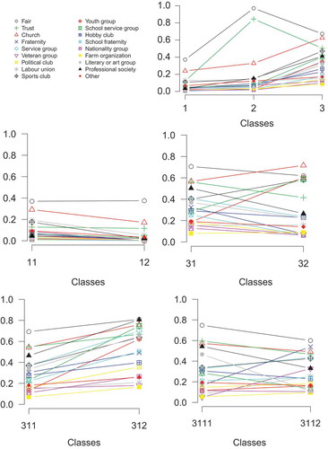
To interpret the tree, the profile plots of every split, as shown in Figure 2, can be investigated. The first split shows three classes, of which the first has a low probability on all variables, the second displays a low probability on participation in all voluntary organizations and very high probabilities on the variables fair and trust, while the class 3 displays relative high probabilities on participation in the voluntary organizations and rather high probabilities for fair and trust. Subsequently, the first and class 3 are split further, while the second is not. The class 1 is split into classes with low and with very low probabilities on all variables, while the class 3 is split into two classes with preferences for different voluntary organizations (e.g., a high probability for being part of a professional organization in class 31 versus a high probability for being part of a youth group in class 32). Subsequently, class 31 is split further, in classes 311 and 312, which seem to differ mainly in participation in all voluntary organizations. The final split in classes 3111 and 3112 results in classes which differ again in preferences for different voluntary organizations (e.g., a high probability for being part of a literary or art group in class 3111 versus a high probability for being part of a fraternity in class 3112).

Figure 2 Profile plots of a LCT with a root of three classes on social capital.

After building the tree, the three-step procedure is used to investigate the class differences in terms of the continuous variable age and the dichotomous variable gender. That is, we compare the mean age and the gender distribution between the newly formed classes at each split.

Within R, this is done with the exploreTree function. The argument resTree refers to the R-object containing the results of the LCT analysis, the argument dirTreeResults indicates the directory with the results of the LCT analysis, and ResultsFolder specifies where the results of the three-step analysis should be written (here the exploreTree_Social_Capital folder). The analysis argument indicates whether the external variables are “dependent” on the class membership (as is the case in this example) or “covariates” predicting the class membership (as will be shown in the next example). The names, number of response options, and scale types of the external variables age and sex are indicated by the remaining arguments. Note that setting the number of response options equal to one implies that the variable is treated as continuous. The final argument called method determines the correction method and indicates whether the ML or BCH method should be used.

explTree.SC3 = exploreTree (resTree = Results.SC3,

dirTreeResults =

paste0(getwd (), “/Results_Social_Capital”),

ResultsFolder = “exploreTree_Social_Capital”,

analysis = “dependent”,

Covariates = c(“sex”, “age”),

sizeMlevels = c(2, 1),

mLevels = c(“ordinal”, “continuous”),

method = “bch”)

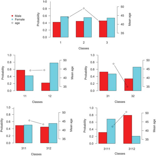
The results of the three-step method are visually displayed in Figure 3. From this figure, we can conclude that after the first split the age is highest in class 2 and lowest in class 3, while the percentage of (wo)men is about the same in every class, though still significantly different according to a Wald test (W(2)$=$11.690, p$<$0.05). After the split of class 1, there is no noticeable difference in age between classes 11 and 12, as can be seen in Figure 3 and this is also confirmed by a Wald test (W(1)$=$0.040, p$=$0.84). There is a significant difference in the percentage of (wo)men between classes 11 and 12 (W(1)$=$192.656, p$<$0.05). It seems that class 12, with very low probabilities on all variables, mainly consists of women, while class 11, with low probabilities on all variables, consists of more men. The split of class 3 results in two classes which differ both on average age (W(1)$=$258.988, p$<$0.05) and percentage of (wo)men (W(1)$=$46.090, p$<$0.05). The difference in age between these classes (and the direction of the difference) could be explained by the fact that class 31 contains more respondents that are part of a professional organization, while class 32 contains more respondents that are part of a youth group and the latter are a lot younger than the former. The difference in the proportion of men and women is not that large in class 31 (53% men and 47% women), while this difference is quite profound in class 32 (34% men and 66% women). The next split in classes 311 and 312 does not result in any significant differences on age (W(1)$=$2.090, p$=$0.15) and percentage of (wo)men (W(1)$=$0.746, p$<$0.39), while the final split in classes 3111 and 3112 results in differences in both age (W(1)$=$116.411, p$<$0.05) and percentage of (wo)men (W(1)$=$42.934, p$<$0.05).

Example 2: Mood Regulation

The second data set stems from a momentary assessment study by Crayen, Eid, Lischetzke, Courvoisier, and Vermunt (2012). It contains eight mood assessments per day during a period of 1 week among 164 respondents (88 women and 76 men, with a mean age of 23.7, SD = 3.31). Respondents answered a small number of questions on a handheld device at pseudo-random signals during their waking hours. The delay between adjacent signals could vary between 60 and 180 min (M [SD] = 100.24[20.36] min, min = 62 min, max = 173 min). Responses had to be made within a 30-min time window after the signal, and were otherwise counted as missing. On average, the 164 participants responded to 51 (of 56) signals (M [SD] = 51.07 [6.05] signals, min = 19 signals, max = 56 signals). In total, there were 8374 non-missing measurements.

Figure 3 Results of the three-step procedure for gender and age on the LCT on social capital.

At each measurement occasion, participants rated their momentary mood on an adapted short version of the Multidimensional Mood Questionnaire (MMQ). Instead of the original monopolar mood items, a shorter bipolar version was used to fit the need for brief scales. Four items assessed pleasant-unpleasant mood (happy-unhappy, content-discontent, good-bad, and well-unwell). Participants rated how they momentarily felt on a 4-point bipolar intensity scales (e.g., very unwell, rather unwell, rather well, very well). For the current analysis, we focus on the item well-unwell. Preliminary analysis of the response-category frequencies showed that the lowest category (i.e., very unwell) was only chosen in approximately 1% of all occasions. Therefore, the two lower categories were collapsed together into one unwell category. The following LCGT model is based on the recoded item with three categories (conform Crayen et al. (2012)). For the subsequent bias-adjusted three-step tree procedure, three personality traits (neuroticism, extraversion, and conscientiousness) are used to predict latent class membership. These traits were assessed with the German NEO-FFI (Borkenau & Ostendorf, 2008) before the momentary assessment study started. The score of each trait is a mean of 12 items per dimension, ranging from 0 to 4. For this example, we estimate the three-step model of every split with the ML method (Vermunt, 2010), as this is the preferred option when the external variables as used as covariates predicting class membership (Bakk & Vermunt, 2016).

Also, this data set is part of the LCTpackage and can be loaded in the R-environment as shown below. The dependent variable called “well” needs to be recoded as a factor to be modeled as an ordinal variable. Note furthermore that this data set is organized in long format and thus contains multiple rows (one for each time point) per respondent.

• data(“MoodRegulation”)

  # Make the items factors, to be ordinal in the model

• MoodRegulation[,“well”] = as.factor (MoodRegulation[, “well”])

For the analysis, we used a LCG model based on an ordinal logit model. The time variable was the time during the day, meaning that we model the mood change during the day. There was a substantial difference between a tree based on a second- or a third-degree polynomial, which indicates that developments are better described by cubic growth curves than quadratic growth curves (see also the trajectory plots in Figure 5). Because there was no substantial difference between a tree based on a third- or a fourth-degree polynomial, a third-degree polynomial was used. Based on the relative improvement of the log-likelihood, BIC, and AIC (Table 2), it seems sensible to start with three classes at the root of the tree to three. This model can be estimated in R with the LCGT function presented below. The argument dependent should be provided with the name of the dependent variable (in this case well) and the argument independent should be provided with the names of the time variables that are part of the polynomial (in this case, a third-order polynomial). The LCGT function also requires the argument caseid specifying the identifier linking the multiple records of the same respondent. Furthermore, the argument levelsDependent needs to be provided with the number of response options of the dependent variable, while the results are written to the newly created folder Results_MoodRegulation_3 within the current working directory. The last argument is used again to retain the variables for the three-step analysis.

Table 2 Log-Likelihood, Number of Parameters, BIC, AIC, and Relative Improvement of the Log-Likelihood, BIC, and AIC of a Traditional LC Growth Model with 1 to 9 Classes

	$logL$	$P$	$BIC$	$AIC$	$R{I}_{logL}$	$R{I}_{BIC}$	$R{I}_{AIC}$
1	−7199	4	14424	14408
2	−6741	9	13538	13504
3	−6578	14	13244	13191	0.355	0.333	0.347
4	−6516	19	13149	13077	0.137	0.107	0.126
5	−6471	24	13091	13001	0.097	0.065	0.085
6	−6443	29	13064	12956	0.062	0.030	0.050
7	−6424	34	13058	12931	0.040	0.007	0.028
8	−6415	39	13069	12923	0.021	−0.013	0.008
9	−6404	44	13078	12914	0.024	−0.010	0.011

Results.MR3 = LCGT(Dataset = MoodRegulation,

LG = G,

maxClassSplit1 = 3,

dependent = “well”,

independent = c(“time_cont”,

“time_cont2”,

“time_cont3”),

caseid = “UserID”,

levelsDependent = 3,

resultsName = “_MoodRegulation_3”,

nKeepVariables = 3,

namesKeepVariables = c(“Neuroticism”,

“Extraversion”,

“Conscientiousness”))

The layout and size of the LCGT with three root classes is presented in Figure 4 and its growth curve plots in Figure 5. The growth plots show that at the root of the tree, the three different classes all improve their mood during the day. They differ in their overall mood level, with class 3 having the lowest and class 2 having the highest overall score. Moreover, class 1 seems to be more consistently increasing than the other two classes. These three classes can be split further. Class 1 splits into two classes with both an average score around one, class 11 just above and class 12 just below. Moreover, the increase in class 11 is larger than in class 12. The split of class 2 results in class 21 consisting of respondents with a very good mood in the morning, a rapid decrease until mid-day, and a subsequent increase. In general, the mean score of class 21 is high relative to the other classes. Class 22 starts with an average mean score and subsequently only increases. The splitting of class 3 results in two classes with a below average mood. Both classes increase, class 31 mainly in the beginning and class 32 mainly at the end of the day.

Figure 4 Layout of a LCT with a root of three classes on mood regulation.

Figure 5 Profile plots of a LCGT on mood regulation with a root of three classes.

After building the tree, the three-step procedure is used to investigate the relation of the three personality traits (neuroticism, extraversion, and conscientiousness) with latent class membership. It is investigated to what extent each of the personality traits can predict latent class membership, while controlling for the other traits. The R-code below shows how the exploreTree function (the same as used in the social capital example) can be used for the three-step analysis. The arguments are basically the same as in the previous example, as resTree refers to the R-object containing the results of the LCGT function, dirTreeResults indicates to the directory with the results of the LCGT analysis, and the results of the three-step analysis will be written to the folder exploreTree_MoodRegulation in the current working directory. The analysis argument indicates with the term “covariates” that the external variable should be used as predictors of class membership. The method argument indicates which estimation method to use. By default, this is the BCH method, as was used in the previous example, while in the current example the ML method is used. The last three arguments provide again information on the names, response options, and measurement levels of the covariates at hand.

explTree.MR3 = exploreTree (resTree = Results.MR3,

LG = LG,

dirTreeResults =

paste0(getwd(), “/Results_MoodRegulation_3”),

ResultsFolder = “exploreTree_MoodRegulation”,

analysis = “covariates”,

method = “ml”,

sizeMlevels = rep(1, 3),

Covariates = c(“Neuroticism”,

“Extraversion”,

“Conscientiousness”),

mLevels = rep (“continuous”,))

The results of this three-step LCGT procedure are depicted in two separate figures, as the root of the tree splits into three classes and is more complex than the subsequent splits of the tree. In Figure 6, the results of the tree-step procedure on the first split are displayed for every variable separately. Each line indicates the probability of belonging to a certain class given the score of one of the personality traits. Note that the probability of belonging to a certain class depends on the combined score of the personality traits. Therefore, the displayed probability for each trait is conditional on the average of the other two traits.

Figure 6 Results of the three-step procedure for the three personality traits on the root of the LCGT on mood regulation.

The first graph of Figure 6 shows that a person with a low score on neuroticism has a relatively high probability of belonging to class 1. However, this probability decreases when neuroticism increases and when a person has a score on neuroticism above three this person is most likely to belong to class 3. Hence, a very neurotic person is likely to display a low overall mood level, while less neurotic persons are most likely to display a mood level that is neither very high nor very low. The second graph of Figure 6 shows that a person with a low score on extraversion has a high probability of belonging to class 1, but when extraversion decreases, so does the probability of belonging to class 1. Respondents with a score of 3.7 or higher on extraversion most likely belong to class 2. Hence, a very extravert person likely has a high overall positive mood level, while less extravert persons are most likely to display a positive mood level that is neither very high nor very low. The last graph of Figure 6 shows that a person with a low score on conscientiousness is most likely to belong to class 3. When a person’s score on conscientiousness is above 1.6, this person is more likely to belong to class 1. This indicates that persons with a low conscientiousness are most likely to display a non-positive overall mood level, while persons with a high conscientiousness are most likely to display an average mood level.

Figure 7 shows the results of the tree-step analysis for each of the three splits at the second level of the LCGT on mood regulation. Each graph shows the results for one split and every line indicates the probability of belonging to the first and largest class of the split corresponding to the personality trait in question (again conditional on an average score of the other two personality traits). The probability of belonging to the class 2 is not displayed, but when there are only two classes, this is by definition the complement of the probability of belonging to the class 1. Note that these results are conditional on being in class 1, 2, or 3.

Figure 7 Results of the three-step procedure for the three personality traits on the second level of the LCGT on mood regulation.

The first graph of Figure 7 shows that the probability of belonging to class 11 increases mainly with a low score on conscientiousness and/or a high score on extraversion. The effect of neuroticism is less strong, but a higher score does indicate a higher probability of belonging to class 11. Hence, low conscientiousness, high extraversion, or high neuroticism indicate a higher probability that respondents’ mood is in general slightly more positive. The second graph of Figure 7 shows that class membership is not really influenced by different scores of the personality traits, but only when extraversion is very high. Hence, the three personality trait are not good predictors for whether a respondent of class 2 has a somewhat continuously rising mood, or a higher, but more fluctuating mood. The third graph of Figure 7 shows that a person with a low neuroticism, low conscientiousness, and/or high extraversion is most likely to be a member of class 31, while a person with a high neuroticism, high conscientiousness, or low extraversion is most likely to be a member of class 32. Hence, a person with a high score on neuroticism or conscientiousness or a low score on extraversion is more likely to have a more negative overall mood than a person with a low score on neuroticism or conscientiousness or a high score on extraversion.

Discussion

LC and LCG models are used by researchers to identify (unobserved) subpopulations within their data. Because the number of latent classes retrieved is often large, the interpretation of the classes can become difficult. That is, it may become difficult to distinguish meaningful and less meaningful subgroupings found in the data set at hand. LCT modeling and LCGT modeling have been developed to deal with this problem. However, assessing and interpreting the classes in LC and LCG models is usually just the first part of an analysis. Typically, researchers are also interested in how class membership is associated with other, external variables. This is commonly done by performing a second step in which respondents are assigned to the estimated classes and a third step in which the relationships of interest are studied using the assigned classes, where in the latter step one may also take the classification errors into account to prevent possible bias in the estimates. In this paper, we have shown how to adapttransform the bias-adjusted three-step LC procedure to be applicable also in the context of LCT modeling and moreover introduced the LCTpackage.

The bias-adjusted three-step approach for LCT modeling has been illustrated with two empirical examples, one in which external variables are treated as distal outcomes of class membership and one in which external variables are used as predictors of class membership. The three-step approach, as presented in this paper, yields results per split of the LCT. An alternative could be to decide on the final classes of the LCT, and subsequently apply the three-step procedure to these end node classes simultaneously. This comes down to applying the original three-step approach, but neglecting that a LCT is built with sequential splits. Since these sequential splits are one of the main benefits of LCTs that facilitate the interpretation of the classes, the approach chosen here makes full use of the structure of a LCT. Another alteration could be to use modal assignment in step two instead of proportional assignment, which implies that one will have less classification errors. However, we do not expect this will matter very much since in the third step one takes into account the classification errors introduced by the classification method used (Bakk, Oberski, & Vermunt, 2014).

The bias-adjusted three-step method has become quite popular among applied researchers, but the basis of this method, the LC and LCG models, are not easy at all for applied researchers (Van De Schoot, Sijbrandij, Winter, Depaoli,& Vermunt, 2016). The tree approach facilitates the use of these models, which can lead to more interpretable and more meaningful classes. With the addition of the bias-adjusted three-step method for LCTs and LCGTs, these classes can now also be related to external variables.

Additional information

Funding

This work was supported by the Nederlandse Organisatie voor Wetenschappelijk Onderzoek [453-10-002].

Notes

¹ This is comparable with how some distance based clustering approaches work (e.g., divisive hierarchical clustering). However, these yield a hard-partitioning at each split meaning that uncertainty about cluster memberships is not taken into account. LCT models do so, as will be shown in the method section.

References

- Bakk, Z., Oberski, D. L., & Vermunt, J. K. (2014). Relating latent class assignments to external variables: Standard errors for correct inference. Political Analysis 22(4): 520–540. mpu003. doi:10.1093/pan/mpu003.
- Bakk, Z., Oberski, D. L., & Vermunt, J. K. (2016). Relating latent class membership to continuous distal outcomes: Improving the ltb approach and a modified three-step implementation. Structural Equation Modeling: A Multidisciplinary Journal, 23(2), 278–289. doi:10.1080/10705511.2015.1049698
- Bakk, Z., Tekle, F. B., & Vermunt, J. K. (2013). Estimating the association be- tween latent class membership and external variables using bias-adjusted three-step approaches. Sociological Methodology, 43(1), 272–311. doi:10.1177/0081175012470644
- Bakk, Z., & Vermunt, J. K. (2016). Robustness of stepwise latent class modeling with continuous distal outcomes. Structural Equation Modeling: A Multidisciplinary Journal, 23(1), 20–31. doi:10.1080/10705511.2014.955104
- Bolck, A., Croon, M., & Hagenaars, J. (2004). Estimating latent structure models with categorical variables: One-step versus three-step estimators. Political Analysis, 12(1), 3–27.
- Borkenau, P., & Ostendorf, F. (2008). NEO-FFI: NEO-Fünf-Faktoren-inventar nach costa und mccrae, manual. Göttingen, Germany: Hogrefe.
- Clogg, C. C. (1995). Latent class models. In Handbook of statistical modeling for the social and behavioral sciences (pp. 311–359). New York, NY: Plenum Press.
- Crayen, C., Eid, M., Lischetzke, T., Courvoisier, D. S., & Vermunt, J. K. (2012). Exploring dynamics in mood regulation—Mixture latent markov modeling of ambulatory assessment data. Psychosomatic Medicine, 74(4), 366–376. doi:10.1097/PSY.0b013e31825474cb
- Dayton, C. M., & Macready, G. B. (1988). Concomitant-variable latent-class models. Journal of the American Statistical Association, 83(401), 173–178. doi:10.1080/01621459.1988.10478584
- Goodman, L. A. (1974). Exploratory latent structure analysis using both identifiable and unidentifiable models. Biometrika, 61(2), 215–231. doi:10.1093/biomet/61.2.215
- Hagenaars, J. A. (1990). Categorical longitudinal data: Log-linear panel, trend, and cohort analysis. Califorina: Sage Newbury Park.
- Lazarsfeld, P. F., & Henry, N. W. (1968). Latent structure analysis. Boston, MA: Houghton Mifflin.
- McCutcheon, A. L. (1987). Latent class analysis (No. 64). Sage.
- Muthén, B. (2004). Latent variable analysis. In D. Kaplan (Ed.), The Sage handbook of quantitative methodology for the social sciences (pp. 345–368). Thousand Oaks, CA: Sage Publications.
- Owen, A. L., & Videras, J. (2009). Reconsidering social capital: A latent class approach. Empirical Economics, 37(3), 555–582. doi:10.1007/s00181-008-0246-6
- R Core Team. (2016). R: A language and environment for statistical com- puting [Computer software manual]. Vienna, Austria. Retrieved from https://www.R-project.org/
- Van De Schoot, R., Sijbrandij, M., Winter, S. D., Depaoli, S., & Vermunt, J. K. (2016). The grolts-checklist: Guidelines for reporting on latent trajectory studies. Structural Equation Modeling: A Multidisciplinary Journal, 24(3), 451–467.
- van Den Bergh, M., Schmittmann, V. D., & Vermunt, J. K. (2017). Building latent class trees, with an application to a study of so- cial capital. Methodology, 13(Supplement 1), 13–22. Retrieved from. doi:10.1027/1614-2241/a000128
- van Den Bergh, M., van Kollenburg, G. H., & Vermunt, J. K. (2018). Deciding on the starting number of classes of a la- tent class tree. Sociological Methodology, 48(1), 303–336. Retrieved from. doi:10.1177/0081175018780170
- van Den Bergh, M., & Vermunt, J. K. (2017). Building latent class growth trees. Structural Equation Modeling: A Multidisciplinary Journal, 1–12. Retrieved from. doi:10.1080/10705511.2017.1389610
- Van der Heijden, P. G., Dessens, J., & Bockenholt, U. (1996). Estimating the concomitant-variable latent-class model with the em algorithm. Journal of Educational and Behavioral Statistics, 21(3), 215–229. doi:10.3102/10769986021003215
- Van der Palm, D. W., van der Ark, L. A., & Vermunt, J. K. (2015). Divisive latent class modeling as a density estimation method for categorical data. Journal of Classification, 33(1), 52–72.
- Vermunt, J. K. (2010). Latent class modeling with covariates: Two improved three-step approaches. Political analysis, 18(4), 450–469.
- Vermunt, J. K., & Magidson, J. (2016). Technical guide for latent gold 5.0: Basic, advanced, and syntax.
- Yamaguchi, K. (2000). Multinomial logit latent-class regression models: An analysis of the predictors of gender-role attitudes among japanese women. American Journal of Sociology, 105(6), 1702–1740. doi:10.1086/210470