Robustness of Individual Score Methods against Model Misspecification in Autoregressive Panel Models

Abstract

Different methods to obtain individual scores from multiple item latent variable models exist, but their performance under realistic conditions is currently underresearched. We investigate the performance of the regression method, the Bartlett method, the Kalman filter, and the mean score under misspecification in autoregressive panel models. Results from three simulations show different patterns of findings for the mean absolute error, for the correlations between individual scores and the true scores (correlation criterion), and for the coverage in our settings: a) all individual score methods are generally quite robust against the chosen misspecification in the loadings, b) all methods are similarly sensitive to positively skewed as well as leptokurtic response distributions with regard to the correlation criterion, c) only the mean score is not robust against an integrated trend component, and d) coverage for the mean score is consistently below the nominal value.

Keywords:

• Individual score/factor score methods
• Kalman filter
• longitudinal autoregressive models
• model misspecification

In psychological research, we often aim at understanding individual development with regard to some latent variable such as depression, competencies, or emotional quantities. The question of how we can obtain scores for latent variables that reliably and validly represent the construct we want to measure guides efforts in latent variable modeling. Most of the popular longitudinal models (e. g., multilevel models or autoregressive (AR) models) yield model parameters such as averages, coefficients of variation or regression coefficients, but they do not directly provide information on individual trajectories. Individual score estimates, sometimes also referred to as predictions, allow us to locate persons on an underlying latent variable (often a normally distributed random latent variable), and, thus, to track them for reasons of monitoring, diagnosis, or prognosis. However, as opposed to parameters of longitudinal models themselves, methods to obtain individual scores are comparatively underresearched, especially in regard to model misspecification.

Research on individual score methods and their performance has a long history, beginning in the last century. Most of the research on individual score methods conducted before the turn of the millennium deals with the performance of individual score methods in the context of exploratory factor analysis (e. g., Horn, 1965), where one of the leading questions was centered around the indeterminacy of individual scores. For a summary of the history of individual score methods and the problem of factor indeterminacy, see for instance Steiger (1979), Acito and Anderson (1986), and Steiger (1996).

Due to the development and spreading of latent variable modeling during the past decades, the focus of recent research on individual score methods has shifted away from their primary use in exploratory factor analyses towards their use in full latent variable models. In one strand of research, individual score methods are investigated with respect to their performance in multistep procedures (e. g., Croon, 2002; Devlieger, Mayer, & Rosseel, 2016; Devlieger & Rosseel, 2017; Hoshino & Bentler, 2013; Skrondal & Laake, 2001). Those approaches have in common that individual scores are first obtained based on a measurement model before they are used to study structural relationships between latent variables. A related strand of research focuses on the role of covariates in individual score modeling (Curran, Cole, Bauer, Hussong, & Gottfredson, 2016; Curran, Cole, Bauer, Rothenberg, & Hussong, 2018). Other applications of individual scores in quantitative psychology include propensity score analysis (Raykov, 2012; for problems of this approach see Lockwood & McCaffrey, 2016), latent interaction modeling (Schumacker, 2002), residual analysis (e. g., Bollen & Arminger, 1991; Coffman & Millsap, 2006), and integrative data analysis, where individual scores are used for secondary analyses of multiple pooled raw datasets (e. g., Curran & Hussong, 2009).

Most of the previous research on individual score method performance is either not tailored to focus on the individuals themselves (e. g., when individual scores are used to study structural relationships between latent variables) or their performance is studied under ideal conditions, that is, when all of the model assumptions are perfectly met. However, in practice, such ideal situations hardly ever exist and findings require further supportive or contradictory evidence (Wackwitz & Horn, 1971, p. 406). When analyzing real data, our models are usually somewhat misspecified, that is, the model that is used for data analysis differs from the model that generated the data. To account for this fact, the goal of our article is to investigate the robustness of different individual score methods against model misspecification in a series of simulation studies. We connect to previous research by choosing similar design factors and features. We extend previous studies by focusing on individuals (rather than on average model parameters) and by taking a longitudinal perspective. To account for the longitudinal structure, we use an autoregressive panel model, where one latent variable measured by multiple indicators predicts the value of the same variable at the next time point. Panel models are often characterized by having rather small numbers of measurement occasions but many individuals and are used, for instance, in clinical (e. g., Luoma et al., 2001; Nolen-Hoeksema, Girgus, & Seligman, 1992) or educational (e. g., Compton, Fuchs, Fuchs, Elleman, & Gilbert, 2008; Lowe, Anderson, Williams, & Currie, 1987; Osborne & Suddick, 1972) contexts.

Our paper is structured as follows. First, we present four common individual score methods: the individual mean score, the regression method, the Bartlett method, and the Kalman filter. As we will show in more detail later on, the individual mean score is usually directly computed by the researchers themselves, whereas the other methods require some latent variable model¹ and are part of most standard software packages for latent variable modeling. The mean score is the most restrictive method as it does not incorporate any estimated model parameters but implicitly assumes an equal weighting of perfectly measured responses. If these assumptions are met, for instance, because the measurement with the corresponding instrument has been shown to be psychometrically sound, reliable, and valid, it is perfectly fine to use the sum or mean score. If, however, good psychometric properties have not been shown, the implicit assumptions may be violated. The Bartlett method does not incorporate structural model parameters (except for mean structures) but only considers loadings and error variances from the measurement model. The regression method as well as the Kalman filter incorporate structural model parameters in addition to measurement model parameters, but they slightly differ in the extent to which that information is used: the Kalman filter only incorporates information up to the current time point, not from future time points as the regression method, which exploits all available information to estimate the individual scores. Next, we investigate the robustness of the selected methods against model misspecification in three simulation studies. The models are misspecified with regard to the loadings (Study 1), the distributional assumptions of the responses (Study 2), and the structural model (Study 3). In Study 3, we use an autoregressive model with an integrated trend to generate the data but estimate the model based on an autoregressive model without a trend as in Studies 1 and 2. To investigate the performance of different individual score methods under model misspecification in AR panel models, we rely on parameters similar to those by Muthén and Muthén (2002) or we use misspecifications as used in recent studies. We thus connect our research to the most current research of individual score methods, rather than pursuing a “testing the limits”, fully-blown simulation study that focuses on one selected type of misspecification.

We expect that the mean score and the Bartlett method should be more sensitive to misspecifications as specified in Studies 1 and 2. These studies will show whether the incorporation of longitudinal information as done by the regression method and the Kalman filter can compensate for misspecification in the measurement model. The regression method and the Kalman filter might be prone to an omitted linear trend as specified in Study 3. Also the mean score may show worse performance in Study 3 as it does not account for any structural information (i. e., a trend).

By examining the robustness of different, easily accessible individual score methods against common types of model misspecification, we make a step towards determining the appropriateness of individual score methods in a wide range of empirical situations. We investigate what we gain or lose in terms of performance when we apply one or the other method in controlled but realistic scenarios.

Individual scores

For the purpose of the present paper and in line with Hardt, Hecht, Oud, and Voelkle (2019), we consider an individual score as a realization of a normally distributed random latent variable that conceptually represents a psychological construct. Let any construct (e. g., intelligence, depression, positive/negative affect, etc.) be measured by $i=1,\dots ,I$ multiple indicators (synonym: items), for which we can observe a response $y_i$. Further, let $c=1,\dots ,C$ be the running index of the latent variables representing the constructs of interest with $C$ being the total number of constructs. Let ${\mathbf{f}}_j$ be the vector of the $C$ latent variable values for $j=1,\dots ,J$ individuals. The common factor model establishes the following linear relationship between the responses and the latent variables:

(1) $\underset{I\times 1}{y_j}=\underset{I\times 1}{v}+\underset{I\times C}{\Lambda }\cdot \underset{C\times 1}{f_j}+\underset{I\times 1}{{{\rm E}}_j},$(1)

where ${\mathbf{y}}_j$ is a vector of the manifest responses across items for person $j$, $\mathit{v}$ is a vector of item intercepts, $\mathbf{\Lambda }$ is the loading matrix connecting manifest and latent variables, and ${\text{Epsilon}}_j$ is the vector of error terms in the measurement model, with ${\text{Epsilon}}_j\sim \mathcal{N}(\mathbf{0},\mathbf{\Theta })$, where $\mathbf{\Theta }$ is the variance-covariance matrix of ${\text{Epsilon}}_j$. If, in addition, relations among the latent variables are postulated, those can be expressed by

(2) $\underset{C\times 1}{f_j}=\underset{C\times 1}{\alpha }+\underset{C\times C}{B}\cdot \underset{C\times 1}{f_j}+\underset{C\times 1}{\zeta {}_j},$(2)

where $\alpha$ contains the intercepts of $\mathbf{f}$, $\mathbf{B}$ contains all directed effects among the $C$ latent variables and $\zeta {}_j$ are the structural disturbances for subject $j$ with $\zeta {}_j\sim \mathcal{N}(\mathbf{0},\mathbf{\Psi })$, where $\mathbf{\Psi }$ is the variance-covariance matrix of $\zeta {}_j$.

Because ${\mathbf{f}}_j$ denotes values of latent variables that cannot be directly observed, individual score estimates or predictions ${\hat{\mathbf{f}}}_j$ need to be obtained. In the following paragraph we present several ways to obtain individual score estimates ${\hat{\mathbf{f}}}_j$ from observable responses ${\mathbf{y}}_j$.

Individual score methods

One simple way to obtain individual scores ${\hat{\mathbf{f}}}_j$ is to compute individual sum scores or mean scores for the $C$ latent variables as defined by

(3) $\underset{C\times 1}{{\widehat{f}}_{{\text{SS}}_j}}=\underset{C\times I}{S^{\prime }}\cdot \underset{I\times 1}{y_j},$(3)

where ${\hat{\mathbf{f}}}_{\mathrm{S}{\mathrm{S}}_j}$ denotes individual scores obtained by computing individual sum scores, and $\mathbf{S}$ is a selection matrix that assigns a particular element in ${\mathbf{y}}_j$ to its corresponding construct. Choosing $s_{ic}\in \{0,1\}$ yields sum scores for ${\hat{\mathbf{f}}}_{\mathrm{S}{\mathrm{S}}_j}$, whereas we obtain mean scores by choosing $s_{ic}\in \{0,\frac{1}{I_c}\}$, where $I_c$ denotes the total number of items $I$ measuring one specific construct $c$. If there are no missing values, an individual’s sum score and mean score correlate to one and differ only by their scale. These approaches assume that items are equally strongly related to the latent variables (i. e., all ${\mathbf{\Lambda }}_i=1$) and that they are measured without any error (i. e., all ${\text{Epsilon}}_j=0$). In order to obtain individual confidence intervals, we can use the standard error of measurement according to $SEm=s\cdot \sqrt{1-\mathrm{r}\mathrm{e}\mathrm{l}\mathrm{i}\mathrm{a}\mathrm{b}\mathrm{i}\mathrm{l}\mathrm{i}\mathrm{t}\mathrm{y}}$, where $s$ is the standard deviation of the sum scores or mean scores, respectively, in the sample. One common choice for the reliability is to use Cronbach’s (1951) Alpha, which, just like the unweighted individual mean or sum score, also makes the assumption of equal loadings and therefore is referred to as tau-equivalent reliability (Cho, 2016).

Lessening these assumptions by incorporating the corresponding model parameters in the computation of individual scores yields more sophisticated approaches such as the Bartlett method, the regression method, and the Kalman filter. According to the Bartlett method (Bartlett, 1937), an individual score is given by

$\underset{C\times 1}{{\widehat{f}}_{{\text{B}}_j}}={(\underset{C\times I}{{\Lambda }^{\prime }}\cdot \underset{I\times I}{{\Theta }^{-1}}\cdot \underset{I\times C}{\Lambda })}^{-1}\cdot \underset{C\times I}{{\Lambda }^{\prime }}\cdot \underset{I\times I}{{\Theta }^{-1}}\cdot (\underset{I\times 1}{y_j}-\underset{I\times 1}{{\mu }_{\text{y}}})+\underset{C\times 1}{\alpha },(4)$

where ${\mu }_{\mathrm{y}}$ are the model implied means for $\mathbf{y}$ as computed by $\mathbf{\Lambda }\cdot \alpha$. In order to obtain standard errors, we can take the square root of the diagonal elements of the estimation error variance-covariance matrix $\mathbf{P}=\mathbb{E}[(\hat{\mathbf{f}}-\mathbf{f})\cdot (\hat{\mathbf{f}}-\mathbf{f}{)}^{\prime }]$ (e. g., Oud, van Den Bercken, & Essers, 1990), with $\hat{\mathbf{f}}$ representing the individual score estimates obtained by a particular method and $\mathbf{f}$ representing the true scores of the latent variables. For the Bartlett method, ${\mathbf{P}}_{\mathrm{B}}=({\mathbf{\Lambda }}^{\prime }\cdot {\mathbf{\Theta }}^{-1}\cdot \mathbf{\Lambda }{)}^{-1}$. As we can see, only the measurement model components $\mathbf{\Lambda }$ and $\mathbf{\Theta }$ enter the computation, whereas structural components are ignored.

This is different in the regression method (Thomson, 1938; Thurstone, 1934), which uses

(5) $\underset{C\times 1}{{\widehat{f}}_{{\text{R}}_j}}=\underset{C\times C}{\Phi }\cdot \underset{C\times I}{{\Lambda }^{\prime }}\cdot \underset{I\times I}{{\Sigma }^{-1}}\cdot (\underset{I\times 1}{y_j}-\underset{I\times 1}{{\mu }_{\text{y}}})+\underset{C\times 1}{\alpha }$(5)

as an estimate of ${\mathbf{f}}_j$, where $\mathbf{\Phi }$ is the variance-covariance matrix of the latent variables $\mathbf{f}$. For the regression method, ${\mathbf{P}}_{\mathrm{R}}=\mathbf{\Phi }\cdot [\mathbf{I}+({\mathbf{\Lambda }}^{\prime }\cdot {\mathbf{\Theta }}^{-1}\cdot \mathbf{\Lambda })\cdot \mathbf{\Phi }{]}^{-1}$. By capturing temporal dependencies among the latent variables in $\mathbf{\Phi }$, the regression method allows us to incorporate longitudinal structural information.

The same is true for the Kalman filter (Kalman, 1960), which is an inherently longitudinal approach and considered to be an optimal method for online individual score estimation (e. g., Hardt et al., 2019; Oud et al., 1990) in a longitudinal context. The Kalman filter involves two steps: in the first step (prediction step), the individual score ${\hat{\mathbf{f}}}_{\mathrm{K}{\mathrm{F}}_{j,t|t-1}}$ at time point $t$ is predicted by the individual score at the previous time point $t-1$ yielding

(6) $\underset{C\times 1}{{\widehat{f}}_{{\text{KF}}_{j,t|t-1}}}=\underset{C\times 1}{\alpha }+\underset{C\times C}{B}\cdot \underset{C\times 1}{{\widehat{f}}_{{\text{KF}}_{j,t-1|t-1}}},$(6)

where $\mathbf{B}$ denotes the transition matrix, which connects $\hat{\mathbf{f}}$ over time. It contains autoregressive parameters in the diagonal and, for $C>1$, cross-lagged effects between $\mathbf{f}$ in the off-diagonals. Thus, the diagonal elements of $\mathbf{B}$ reflect the strength of the relationship of a given construct between adjacent measurement occasions: the closer the absolute values are to one, the stronger the relationship and the better the prediction of $\hat{\mathbf{f}}$ at time point $t$ by $\hat{\mathbf{f}}$ at $t-1$. With the arrival of data from the new measurement at time point $t$ the prediction from time point $t-1$ is updated (update step) according to

(7) $\underset{C\times 1}{{\widehat{f}}_{{\text{KF}}_{j,t|t}}}=\underset{C\times 1}{{\widehat{f}}_{{\text{KF}}_{j,t|t-1}}}+\underset{C\times I}{K_{t|t}}\cdot (\underset{I\times 1}{y_{jt}}-\underset{I\times 1}{{\widehat{y}}_{j,t|t-1}}),$(7)

with ${\hat{\mathbf{y}}}_{j,t|t-1}$ being the responses predicted by $\mathbf{\Lambda }\cdot {\hat{\mathbf{f}}}_{\mathrm{K}{\mathrm{F}}_{j,t|t-1}}$. The Kalman gain, ${\mathbf{K}}_{t|t}$, determines how strongly the new measurement is weighted as compared to the prediction based on the previous time point and is defined by

(8) $\underset{C\times I}{K_{t|t}}=\underset{C\times C}{P_{{\text{KF}}_{t|t-1}}}\cdot \underset{C\times I}{{\Lambda }^{\prime }}\cdot {(\underset{I\times C}{\Lambda }\cdot \underset{C\times C}{P_{{\text{KF}}_{t|t-1}}}\cdot \underset{C\times I}{{\Lambda }^{\prime }}+\underset{I\times I}{\Theta })}^{-1},$(8)

where ${\mathbf{P}}_{\mathrm{K}{\mathrm{F}}_{t|t-1}}$ is the predicted Kalman estimation error as given by ${\mathbf{P}}_{\mathrm{K}{\mathrm{F}}_{t|t-1}}=\mathbf{B}\cdot {\mathbf{P}}_{\mathrm{K}{\mathrm{F}}_{t-1|t-1}}\cdot {\mathbf{B}}^{\prime }+\mathbf{\Psi }$. The updated Kalman estimation error is defined by ${\mathbf{P}}_{\mathrm{K}{\mathrm{F}}_{t|t}}=(\mathbf{I}-{\mathbf{K}}_{t|t}\cdot \mathbf{\Lambda })\cdot {\mathbf{P}}_{\mathrm{K}{\mathrm{F}}_{t|t-1}}$, where $\mathbf{I}$ is the identity matrix. Note that the index for the time point in the Kalman filtering approach goes from $t=2$ to $T$, where $T$ denotes the total number of measurement occasions. At $t=1$, the Kalman filter can be initialized completely “uninformative” for instance by setting ${\mathbf{f}}_{\mathrm{K}{\mathrm{F}}_{j,1|1}}$ and ${\mathbf{P}}_{\mathrm{K}{\mathrm{F}}_{1|1}}$ to arbitrary values or “informative” by choosing individual score estimates obtained by another individual score method (e. g., the Bartlett method or the regression method, see Oud, Jansen, Van Leeuwe, Aarnoutse, & Voeten, 1999; Hardt et al., 2019; for more comprehensive research on the initial condition specification, see Losardo, 2012).

Simulation studies

Three simulation studies were conducted in order to examine the robustness of the four selected individual score methods against misspecification in the context of an AR(1) panel model. Misspecifications are studied with regard to the loadings (Study 1), the distributional assumptions of the responses (Study 2), and the longitudinal structural model (Study 3). Based on the results we draw conclusions for the use of individual scores in practice.

General setting and procedure

All three simulation studies followed the same steps: data generation, model specification and estimation, computation of individual scores, and analyses of the results. Data generation was different across simulations and will be described for each simulation study separately. The model used for data analysis is always a univariate (i. e., $C=1$) autoregressive panel model of order one, AR(1), in which one latent variable with $I=5$ items is repeatedly measured on $T=5$ equally-spaced measurement occasions for $J=200$ individuals.² All variables are $z$-standardized if not indicated otherwise. Adapting Equations (1) and (2) and assuming a stationary process (see e. g., Hamilton, 1994, pp. 45–46) with ${\beta }_t=\beta$ and measurement invariance across time (i. e., ${\mathbf{\Lambda }}_t=\mathbf{\Lambda }$, ${\mathbf{\Theta }}_t=\mathbf{\Theta }$) yields

(9) ${\mathbf{y}}_{jt}=\mathbf{\Lambda }\cdot f_{jt}+{\text{Epsilon}}_{jt}$(9)

with ${\text{Epsilon}}_{jt}\sim \mathcal{N}($0 $,$ $\mathbf{\Theta }$$)$ for the measurement model and

(10) $f_{jt}=\beta \cdot f_{j,t-1}+{\zeta }_{jt}$(10)

with ${\zeta }_{jt}\sim \mathcal{N}(0,\psi$$)$ for the structural model. The disturbance term ${\zeta }_{jt}$, also called process noise, reflects the degree to which $f_{j,t}$ cannot be predicted by $f_{j,t-1}$. Figure 1 depicts the model used for data analysis as well as the locations of the misspecifications in the simulation studies. After having estimated the models, individual scores are computed according to Equations (3) to (7). Unless stated otherwise, we assumed $\alpha =\mathbf{0}$ and $\mathit{v}=\mathbf{0}$.

FIGURE 1 Conceptual path diagram of an autoregressive model of order one with five observed indicators; the squared areas indicate locations of misspecification as examined in the three simulation studies.

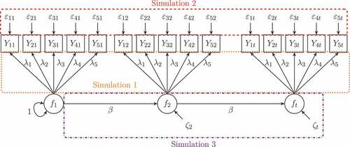
In all three simulation studies, we varied the degree of persistence of the process (referred to as factor beta) to be either 0.25 or 0.75. A parameter of $\beta =0.25$ indicates lower persistence, whereas a parameter of $\beta =0.75$ indicates higher persistence. The different individual score methods are represented as a factor Method which comprises the levels Regression, Bartlett, MeanScore, KFiniR, and KFiniB with the latter two being the Kalman filter initialized with the regression method and the Bartlett method, respectively. As the misspecification in simulation Studies 1 and 2 is located in the measurement model, we varied the average of the loadings (referred to as factor LDm). The average of the loadings was either 0.6 or 0.8. Loadings of 0.8 correspond to a latent variable indicator reliability of $64\mathrm{\%}$ when variables are standardized and can be considered prototypical for loadings in psychological studies (Muthén & Muthén, 2002). The set of loadings with an average value of 0.6 represents situations with less reliable indicators. In practice, loadings are usually not equal across indicators. Hence, loadings for our five observable indicators were chosen in such a way that they approximately followed a normal distribution around the mean. For $LDm=0.8$ conditions, loadings were 0.65, 0.75, 0.80, 0.85, 0.95 and for $LDm=0.6$ conditions, loadings were 0.45, 0.55, 0.60, 0.65, 0.75. In addition, we incorporated the five time points as control factor Time into the analyses of simulation Studies 1 and 2 in order to capture time-specific effects which may emerge in a longitudinal context. Further study specific design factors that relate to the type of misspecification itself are outlined for each simulation study separately.

All steps were replicated $N_{\mathrm{r}\mathrm{e}\mathrm{p}\mathrm{l}}=1,000$ times per condition. If the model converged, we computed individual scores as described before and subsequently evaluated their performance as described next. All analyses were conducted using the package OpenMx (Neale et al., 2016; Boker et al., 2018, version 2.12.2) in the software environment R (R Core Team, 2018, version 3.5.0); individual scores were computed with our own routines. As starting values, we used 0.5 for the loadings, for the process error variance as well as for the autoregression coefficient, and 0.4 for the error variances in the measurement model. For the intercepts in simulation Study 3 we relied on the OpenMx’ default starting value of zero. Further, by specifying lbound = 0.0001 for variances, we ensured that estimates for variances are positive. Regarding model convergence, we relied on OpenMx default values but used the function mxTryHard() with 50 extra attempts to obtain model convergence. In the extra attempts, parameter estimates from the previous attempt are perturbed by random draws from a uniform distribution and then used as starting values for the next attempt.

Outcome criteria

To evaluate the performance of the different individual score methods, we use three criteria: the mean absolute error (MAE), the Fisher-$Z$-transformed correlation between true scores and individual score estimates, and the coverage rate. We use analysis of variance (ANOVA) or logistic regression models to examine variation in the three criteria. In these models, we consider the unique impact of the simulation design and control factors and all possible interactions between them. The MAE is calculated by $N_{\mathrm{r}\mathrm{e}\mathrm{p}\mathrm{l}}^{-1}{\sum }_{r=1}^{N_{\mathrm{r}\mathrm{e}\mathrm{p}\mathrm{l}}}|{\hat{f}}_{j_r}-f_j|$ and is a measure of the absolute discrepancy between the true score and the individual score estimate. It is considered to be among the most appropriate measures when all the data are on the same scale (see Hyndman & Koehler, 2006). The correlation is expressed as $r_{\hat{f}f}$ and it is a relative measure. It describes how well the relative positioning of individuals based on their true scores is maintained by individual score estimates and may thus be considered an index for the individual score reliability. For the MAE and for the correlation criterion, we fit ANOVA models using sums of squares of type III to explain variation in them. The coverage criterion assesses the frequency with which the true score is “captured” by an individual score estimate plus/minus the corresponding 95% confidence interval limits relative to the total number of replications. The confidence intervals are computed by $\mathrm{C}{\mathrm{I}}_{jt}={\hat{f}}_{jt}\pm z_{.975}\cdot S{E}_t$, where $z_{.975}\approx 1.96$ and the standard errors $SE$ at each time point $t$ are obtained based on $SEm,{\mathbf{P}}_{\mathrm{B}},{\mathbf{P}}_{\mathrm{R}},\mathrm{a}\mathrm{n}\mathrm{d}{\mathbf{P}}_{\mathrm{K}{\mathrm{F}}_{t|t}}$ as described before. Ideally, the coverage rate matches the nominal confidence of 95%. Because of its range from 0 to 1, the coverage criterion is further analyzed by means of logistic regression models using dummy coding of the design and control factors as well as all possible interactions between them. In dummy coding, one of the factor levels is chosen as reference category (coded as 0), while each other factor level is represented as dichotomous group indicator with code 1 indicating group membership and 0 otherwise. As for the coverage criterion departures from 0.95 are more important to consider than the mere variation in it, we included an additional Method level with the value 0.95 for each person at each time point and for each condition. This “method” reflects the nominal coverage rate for 95% confidence intervals and is the baseline (“reference category”) for the Method factor. Thus, a regression coefficient for a particular individual score method reflects its departure in coverage from the nominal 95% confidence.³

The three outcome criteria capture very different aspects of individual score method performance. Whereas the MAE and the coverage may be more important in the context of individual diagnostics with predefined diagnostic criteria and thresholds, the correlation criterion may be more important for subsequent (e. g., covariance based) analyses. Note that the MAE and the coverage are calculated for each individual across replications, whereas the correlation criterion is calculated across all individuals per replication, resulting in different numbers of units entering the ANOVA models reported below. Given the extreme power due to the high number of units for the two outcomes (at least 40,000), we only deem factors with both $p<.01$ and an ${\eta }^2$ of at least $.01$ as meaningful in the ANOVA models. In case of such meaningful factors, we further conducted post hoc pairwise comparisons of the factor levels with Bonferroni adjustment of the $p$-values to avoid $\text{Alpha}$ error inflation. We considered significant effects (i. e., $p<.01$) with an effect size of $|d|\ge 0.2$ to be meaningful. For the logistic regression models, we transformed the exponentiated regression coefficients into Cohen’s $d$ according to Borenstein, Hedges, Higgins, and Rothstein (2009, Equation (7.1)) and considered a predictor effect as meaningful if $p<.01$ and $|d|\ge 0.2$. These thresholds correspond to Cohen’s (1988) conventions for small effects and the ${\eta }^2$ threshold is additionally in line with that used by Curran et al. (2016).

Simulation study 1: loadings

Methods

Data generation

Data were generated according to an autoregressive panel model of order one as described before. First, the trajectories of the true scores were generated according to Equation (8). For $t=1$ we drew $J=200$ values from a standard normal distribution. Next, based on the trajectories of the true scores, we generated the response data under the common factor model as given in Equation (9) and with the two sets of loadings with an average of 0.6 and 0.8, respectively, as described before. For this, we multiplied an individual’s true score at a given time point by the loadings and added a measurement residual, ${\text{Epsilon}}_j\sim \mathcal{N}(\mathbf{0},\mathbf{\Theta })$, where the variances in $\mathbf{\Theta }$ are one minus the squared loading, with zeros in the off-diagonals, in order to obtain standardized items without error covariances.

Design and analyses

In order to study the effect of misspecifications in the loadings on individual score methods, we analyzed the data generated with unequal loadings with a model in which the loadings and measurement error variances are assumed to be equal (LDequal). As reference, we compare our results to those obtained for a model with a correct specification of the loadings, that is, when they are estimated freely (LDfree) and subsumed these specifications under the factor LDspec (with the levels LDequal/misspecified vs. LDfree/correct [reference]). In addition, the following aforementioned design and control factors enter the analyses: beta (reference: $\beta =0.75$), LDm (reference: average loading of 0.6), Time (reference: $t=1$), and Method (reference: nominal 95%).

Results

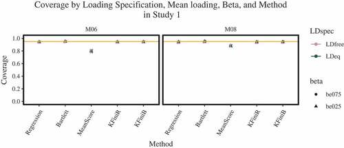
In simulation Study 1, all models converged. With regard to the MAE, we only find a few statistically significant (i. e., $p<.01$) effects (see Table 1), of which only the effect of the average loading design factor LDm can be considered practically meaningful ${\eta }^2=1.1\mathrm{\%}$. Unsurprisingly, this means that a mean loading of 0.8 leads on average to a smaller MAE value than a mean loading of 0.6. Considering the coverage criterion (see Figure 2), only the mean score leads to a meaningfully smaller odds of capturing the true score by the confidence interval as compared to the nominal 0.95 coverage ($OR=0.396,p<.001,d=-0.511$). This effect is more pronounced in $LDm=0.6$ conditions for the mean score than for other individual score methods ($OR=0.527,p<.001,d=-0.353$).

TABLE 1 ANOVA Results for the MAE Criterion for Study 1

term	df	$SS$	$F$	$p$	${\eta }^2$
(Intercept)	1	26.18	4,574.15	<.001	.1
Time	4	0.32	14.00	<.001	.001
Method	4	1.26	54.99	<.001	.005
LDspec	1	0.03	4.86	.028	0
beta	1	0.09	15.15	<.001	0
LDm	1	2.84	496.58	<.001	.011
Time:Method	16	0.76	8.34	<.001	.003
Time:LDspec	4	0.00	0.06	.993	0
Method:LDspec	4	0.07	2.99	.018	0
Time:beta	4	0.08	3.33	.01	0
Method:beta	4	0.12	5.22	<.001	0
LDspec:beta	1	0.00	0.06	.814	0
Time:LDm	4	0.09	3.90	.004	0
Method:LDm	4	0.51	22.45	<.001	.002
LDspec:LDm	1	0.06	9.71	.002	0
beta:LDm	1	0.03	5.05	.025	0
Time:Method:LDspec	16	0.01	0.15	>.999	0
Time:Method:beta	16	0.15	1.62	.055	.001
Time:LDspec:beta	4	0.00	0.01	>.999	0
Method:LDspec:beta	4	0.00	0.04	.997	0
Time:Method:LDm	16	0.31	3.37	<.001	.001
Time:LDspec:LDm	4	0.00	0.04	.997	0
Method:LDspec:LDm	4	0.04	1.74	.138	0
Time:beta:LDm	4	0.02	0.90	.465	0
Method:beta:LDm	4	0.04	1.80	.126	0
LDspec:beta:LDm	1	0.00	0.02	.895	0
Time:Method:LDspec:beta	16	0.00	0.01	>.999	0
Time:Method:LDspec:LDm	16	0.00	0.01	>.999	0
Time:Method:beta:LDm	16	0.04	0.47	.963	0
Time:LDspec:beta:LDm	4	0.00	0.02	.999	0
Method:LDspec:beta:LDm	4	0.00	0.00	>.999	0
Time:Method:LDspec:beta:LDm	16	0.00	0.00	>.999	0
Residuals	39,800	227.76

Note. The design and control factors include Time ($t_1$ $-$ $t_5$), Method (Regression, Bartlett, MeanScore, KFiniR and KFiniB), LDspec (incorrect vs. correct), LDm (mean loading 0.6 vs. 0.8), and beta ($\beta$ $=$ $0.25$ vs. $\beta$ $=$ $0.75$).

FIGURE 2 LDspec = loading specification with LDfree = freely estimated loadings and LDeq = loadings constrained to be equal; M06 = average loading of 0.6, M08 = average loading of 0.8; be025 = $\beta$ of 0.25, be075 = $\beta$ of 0.75. Proportions and confidence intervals for Study 1.

Regarding the correlation criterion (see Table 2), we find the same effect of the average loading on the average $Z$-transformed correlation between the true scores and the estimated individual scores (${\eta }^2=7.4\mathrm{\%}$).

TABLE 2 ANOVA Results for the Correlation Criterion for Study 1

term	df	$SS$	$F$	$p$	${\eta }^2$
(Intercept)	1	2,187.41	758,636.18	<.001	.707
Time	4	8.84	766.65	<.001	.003
Method	4	15.26	1,322.64	<.001	.005
LDspec	1	1.24	428.41	<.001	0
beta	1	3.66	1,268.99	<.001	.001
LDm	1	227.56	78,921.72	<.001	.074
Time:Method	16	13.45	291.54	<.001	.004
Time:LDspec	4	0.01	1.27	.279	0
Method:LDspec	4	1.17	101.46	<.001	0
Time:beta	4	10.08	873.76	<.001	.003
Method:beta	4	4.17	361.31	<.001	.001
LDspec:beta	1	0.01	1.95	.162	0
Time:LDm	4	2.52	218.95	<.001	.001
Method:LDm	4	13.48	1,168.67	<.001	.004
LDspec:LDm	1	9.45	3,278.03	<.001	.003
beta:LDm	1	0.82	284.02	<.001	0
Time:Method:LDspec	16	0.03	0.67	.827	0
Time:Method:beta	16	5.43	117.64	<.001	.002
Time:LDspec:beta	4	0.00	0.25	.91	0
Method:LDspec:beta	4	0.01	1.17	.32	0
Time:Method:LDm	16	2.69	58.27	<.001	.001
Time:LDspec:LDm	4	0.09	8.02	<.001	0
Method:LDspec:LDm	4	7.82	677.85	<.001	.003
Time:beta:LDm	4	0.73	63.43	<.001	0
Method:beta:LDm	4	0.94	81.75	<.001	0
LDspec:beta:LDm	1	0.01	2.75	.097	0
Time:Method:LDspec:beta	16	0.01	0.24	.999	0
Time:Method:LDspec:LDm	16	0.07	1.47	.103	0
Time:Method:beta:LDm	16	1.04	22.56	<.001	0
Time:LDspec:beta:LDm	4	0.04	3.09	.015	0
Method:LDspec:beta:LDm	4	0.01	0.63	.642	0
Time:Method:LDspec:beta:LDm	16	0.03	0.60	.888	0
Residuals	199,800	576.09

Note. The design and control factors include Time ($t_1$ $-$ $t_5$), Method (Regression, Bartlett, MeanScore, KFiniR and KFiniB), LDspec (incorrect vs. correct), LDm (mean loading 0.6 vs. 0.8), and beta ($\beta$ $=$ $0.25$ vs. $\beta$ $=$ $0.75$).

In summary, the effects we found are in line with what we know about the individual score methods’ performance under ideal conditions (i. e., without model misspecification). In turn, this means that loading misspecification, as implemented in this simulation study, neither has a meaningful impact on the MAE nor on the correlation criterion, and that the individual score methods have proven robust against this type of misspecification. However, regardless of the model misspecification, when using the individual mean scores and corresponding confidence intervals, we are testing with a confidence that is actually lower than the nominal confidence. That is, the type I error probability is higher than we assume.

Simulation study 2: response distributions

Methods

Data generation

Data were generated in the same way as described for simulation Study 1 except for the distribution from which the measurement residuals were drawn. In order to generate non-normal response data, measurement residuals were drawn from two different distributions as in Devlieger et al. (2016): for one set of conditions, ${\text{Epsilon}}_j\sim t(3)$ and multiplied by the square root of the diagonal elements in $\mathbf{\Theta }$, resulting in curved response data that are leptokurtic ($M_{\mathrm{k}\mathrm{u}\mathrm{r}\mathrm{t}\mathrm{o}\mathrm{s}\mathrm{i}\mathrm{s}}=9.991,S{D}_{\mathrm{k}\mathrm{u}\mathrm{r}\mathrm{t}\mathrm{o}\mathrm{s}\mathrm{i}\mathrm{s}}=14.416$). For another set of conditions, ${\text{Epsilon}}_j\sim {\chi }^2(1)$ and were multiplied by the square root of the diagonal elements in $\mathbf{\Theta }$, resulting in positively skewed response data ($M_{\mathrm{s}\mathrm{k}\mathrm{e}\mathrm{w}\mathrm{n}\mathrm{e}\mathrm{s}\mathrm{s}}=1.410,S{D}_{\mathrm{s}\mathrm{k}\mathrm{e}\mathrm{w}\mathrm{n}\mathrm{e}\mathrm{s}\mathrm{s}}=0.699$) as may be the case when modeling responses times for instance. In the baseline conditions, ${\text{Epsilon}}_j\sim \mathcal{N}(\mathbf{0},\mathbf{\Theta })$ as before.

Design and analyses

In order to study the effect of non-normally distributed response data on the performance of different individual score methods, we entered the factor Ydistr (representing different response distributions) with the three levels curved, skewed, and normal (reference) into the analyses of the simulation results. In addition, we included beta, LDm, Time, and Method as control and design factors just as before.

Results

In simulation Study 2, all models converged except for up to three replications in conditions with curved response distributions. With regard to the MAE, none of the factors or interactions became significant and explained at least $1\mathrm{\%}$ of the variance in the MAE (see Table 3). That is, the error that we make when estimating individual scores is independent of the design factors, including misspecifications in the response distribution. This is different for the correlation criterion, for which the response distribution (Ydistr) accounts for ${\eta }^2=2.3\mathrm{\%}$ of the variance (see Table 4). Post hoc pairwise analyses yielded strong effects of $|d|=0.535$ for curved response distributions as compared to normal response distributions and of $|d|=0.403$ for skewed response distributions as compared to normal response distributions. The difference between skewed and curved distributions is not meaningful. This result means that individual score methods suffer to the same degree from misspecification in the response distributions in terms of their accuracy in maintaining the relative positioning of individuals. 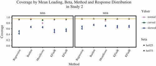Moreover, LDm again turned out to be meaningful (${\eta }^2=6.2\mathrm{\%}$) indicating, as expected, that individual score methods perform better in high average loading conditions than in low average loading conditions. Considering the coverage (see Figure 3), we observe two main findings that are related to the mean score on the one hand, and to the model-based methods on the other. With regard to the mean score, the coverage again results to be meaningfully lower than 0.95 ($OR=0.397,p<.001,d=-0.509$), while keeping the other factors at their baseline. This main effect is strengthened if the average loading is 0.6 as compared to the nominal coverage of 0.95 in a more reliable measurement (LDm = 0.8; OR = 0.526, $p<.001,d=-0.354$). This negative effect is lowered if responses are leptokurtic (OR = 1.810, $p<.001,$ d = 0.327). It is strengthened if they are skewed ($OR=0.310,p<.001,d=-0.646$), particularly, when the average loading is 0.6 as compared to 0.8 ($OR=1.520,p<.001,d=0.231$). With regard to the other, model-based individual score methods, we also find that skewness generally leads to coverage rates meaningfully lower than the nominal 0.95 ($OR$ between 0.125 and 0.157, all $p<.001,d$ between $-1.145$ and $-1.021$) while keeping $\beta$ at 0.75, $LDm$ at 0.8 and $t$ at 1, and that the negative departure from 0.95 is even stronger for $LDm=0.6$ conditions ($OR$ between 0.476 and 0.660, all $p<.001,d$ between $-0.410$ and $-0.229$). The regression method additionally suffers slightly more at $t=2$ (OR = 0.635, $p<.001,d=-0.25$) and $t=4$ ($OR=0.668$, $p<.001,d=-0.222$) from skewed responses. However, note that these time point specific effects for the regression method do not occur in the analyses based on $J=2,000$ individuals. Further, although we do not find a general Kalman filter initialization effect, we observe a few, time point-specific effects: if the responses are skewed at $t=2$ ($OR=0.694$, $p<.001,d=-0.201$), or, in particular, if $LDm=0.6$ at $t=3$ ($OR=0.656$, $p<.001,d=-0.233$) and $t=4$ ($OR=0.692$, $p<.001,d=-0.203$), the Bartlett initialized Kalman filter leads to a coverage below the nominal 0.95. Note that these Kalman filter initialization effects do not occur in the analyses based on $J=2,000$ individuals. Therefore, they are an effect due to bias in the model parameter estimation rather than due to individual score method properties. This will be explained in the discussion. In sum, the results of simulation Study 2 show that all individual score methods are similarly robust against misspecification in the response distribution when their absolute value matters. However, as soon as we consider confidence intervals when the response distributions are skewed, our type I error is inflated. Further, the individual score methods are sensitive to departures from normality when it comes to the relative positioning of individuals.

TABLE 3 ANOVA Results for the MAE Criterion for Study 2

term	df	$SS$	$F$	$p$	${\eta }^2$
(Intercept)	1	30.70	115.64	<.001	.002
Time	4	0.04	0.04	.997	0
Method	4	0.42	0.40	.811	0
Ydistr	2	17.92	33.76	<.001	.001
beta	1	0.09	0.34	.561	0
LDm	1	3.74	14.10	<.001	0
Time:Method	16	0.26	0.06	>.999	0
Time:Ydistr	8	1.69	0.80	.606	0
Method:Ydistr	8	3.53	1.66	.102	0
Time:beta	4	0.09	0.09	.987	0
Method:beta	4	0.11	0.11	.98	0
Ydistr:beta	2	0.09	0.17	.841	0
Time:LDm	4	0.01	0.01	>.999	0
Method:LDm	4	0.30	0.29	.886	0
Ydistr:LDm	2	0.68	1.29	.276	0
beta:LDm	1	0.03	0.12	.732	0
Time:Method:Ydistr	32	1.88	0.22	>.999	0
Time:Method:beta	16	0.15	0.04	>.999	0
Time:Ydistr:beta	8	0.21	0.10	.999	0
Method:Ydistr:beta	8	0.11	0.05	>.999	0
Time:Method:LDm	16	0.12	0.03	>.999	0
Time:Ydistr:LDm	8	14.69	6.92	<.001	.001
Method:Ydistr:LDm	8	2.86	1.35	.215	0
Time:beta:LDm	4	0.03	0.02	.999	0
Method:beta:LDm	4	0.04	0.04	.997	0
Ydistr:beta:LDm	2	0.02	0.04	.96	0
Time:Method:Ydistr:beta	32	0.24	0.03	>.999	0
Time:Method:Ydistr:LDm	32	11.62	1.37	.08	.001
Time:Method:beta:LDm	16	0.04	0.01	>.999	0
Time:Ydistr:beta:LDm	8	7.98	3.76	<.001	.001
Method:Ydistr:beta:LDm	8	3.79	1.78	.075	0
Time:Method:Ydistr:beta:LDm	32	6.01	0.71	.889	0
Residuals	59,700	15,845.70

Note. The design and control factors include Time ($t_1$ $-$ $t_5$), Method (Regression, Bartlett, MeanScore, KFiniR and KFiniB), LDm (mean loading 0.6 vs. 0.8) and beta ($\beta$ $=$ $0.25$ vs. $\beta$ $=$ $0.75$), and response distribution Ydistr (normal, curved and skewed).

TABLE 4 ANOVA Results for the Correlation Criterion for Study 2

term	df	$SS$	$F$	$p$	${\eta }^2$
(Intercept)	1	1,934.60	293,434.79	<.001	.445
Time	4	5.61	212.68	<.001	.001
Method	4	2.54	96.29	<.001	.001
Ydistr	2	102.17	7,748.09	<.001	.023
beta	1	3.77	571.19	<.001	.001
LDm	1	269.99	40,951.68	<.001	.062
Time:Method	16	0.22	2.13	.005	0
Time:Ydistr	8	1.13	21.51	<.001	0
Method:Ydistr	8	1.65	31.25	<.001	0
Time:beta	4	10.47	396.95	<.001	.002
Method:beta	4	4.09	155.23	<.001	.001
Ydistr:beta	2	1.00	75.51	<.001	0
Time:LDm	4	0.15	5.64	<.001	0
Method:LDm	4	16.31	618.56	<.001	.004
Ydistr:LDm	2	1.31	99.72	<.001	0
beta:LDm	1	0.93	140.65	<.001	0
Time:Method:Ydistr	32	1.72	8.15	<.001	0
Time:Method:beta	16	5.45	51.67	<.001	.001
Time:Ydistr:beta	8	0.64	12.04	<.001	0
Method:Ydistr:beta	8	1.42	26.89	<.001	0
Time:Method:LDm	16	0.07	0.66	.836	0
Time:Ydistr:LDm	8	0.30	5.78	<.001	0
Method:Ydistr:LDm	8	0.86	16.34	<.001	0
Time:beta:LDm	4	0.85	32.26	<.001	0
Method:beta:LDm	4	0.98	37.23	<.001	0
Ydistr:beta:LDm	2	0.06	4.38	.013	0
Time:Method:Ydistr:beta	32	1.10	5.24	<.001	0
Time:Method:Ydistr:LDm	32	0.63	2.99	<.001	0
Time:Method:beta:LDm	16	1.03	9.73	<.001	0
Time:Ydistr:beta:LDm	8	0.29	5.58	<.001	0
Method:Ydistr:beta:LDm	8	0.25	4.72	<.001	0
Time:Method:Ydistr:beta:LDm	32	0.42	1.99	.001	0
Residuals	299,650	1,975.58

Note. The design and control factors include Time ($t_1$ $-$ $t_5$), Method (Regression, Bartlett, MeanScore, KFiniR and KFiniB), LDm (mean loading 0.6 vs. 0.8) and beta ($\beta$ $=$ $0.25$ vs. $\beta$ $=$ $0.75$), and response distribution Ydistr (normal, curved and skewed).

FIGURE 3 Ydistr = response distribution; M06 = average loading of 0.6, M08 = average loading of 0.8; be025 = $\beta$ of 0.25, be075 = $\beta$ of 0.75. Proportions and confidence intervals for Study 2.

Simulation study 3: structural misspecification

Methods

Data generation

The goal of simulation Study 3 is to simulate the effect of an unmodeled integrated trend component on individual score methods. Trajectories of true scores are generated according to $f_{jt}=h_t+\beta \cdot f_{j,t-1}+{\zeta }_{jt}$ with ${\zeta }_{jt}\sim \mathcal{N}(0,\psi )$, where $h_t=(t-1)\cdot g$ with $g$ being the slope and $h$ being the trend variable at time $t$. Based on these trajectories of the true scores we then generated the responses according to Equation (9) as before.

Design and analyses

We chose the trend to be either weak with a slope (referred to as factor g) of 0.5 or moderate with a slope of 1. We assess the robustness of individual score methods against ignoring an integrated trend component in an AR(1) model by comparing their performance in an AR(1) model without integrated trend component with their performance in an AR(1) model including an integrated trend component. This trend component can be modeled by an AR(1) process of an additional latent variable (the trend variable) parallel to the AR(1) process of interest while imposing special constraints on this additional process. The two processes are connected by regressing the latent variable of interest on the latent trend variable with the regression coefficient being fixed to one. The variances (initial variance and process noise variance) of the latent trend variable are constrained to zero and the autoregressive coefficient is constrained to 1. The intercept of the latent trend variable is freely estimated from $t=2$ onwards but constrained to be equal across time. All other means and intercepts are constrained to zero. The model-implied mean structure is given in the Appendix. Figure 4 illustrates this model. Example code for specifying this model is provided in the Online Supplemental Material C. The correctly specified model (including the trend; AR1litrend) and the misspecified model (without trend; AR1notrend) were fitted to the same data set, and are subsumed under the factor Model (with the levels AR1notrend/incorrect vs. AR1litrend/correct [reference]) in the following ANOVA and regression models. In addition, we considered beta and Method as design and control factors as before. As simulation Studies 1 and 2 did not yield any meaningful interactions including the LDm conditions, we focused on $LDm=0.8$ in this study. Time was not included as a control factor here because the factor Model already inheres whether the longitudinal structure is appropriately accounted for or not.

FIGURE 4 Conceptual path diagram of an autoregressive model of order one including an integrated trend component, five observed indicators, and measurement invariance assumed as used for simulation Study 3.

Results

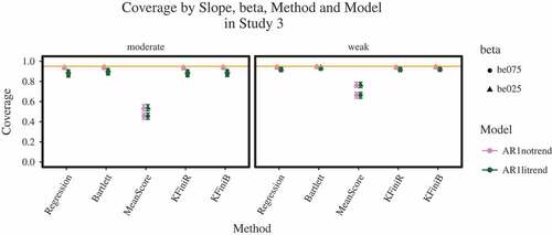
In simulation Study 3, all models converged. For the three outcome criteria, we find different patterns of results, including differences in coverage between the analysis with $J=200$ and $J=2,000$. With regard to the MAE, we find a meaningful main effect for Method (${\eta }^2=18.5\mathrm{\%}$) as well as meaningful effects for the interactions between Method and slope (${\eta }^2=2.9\mathrm{\%}$) and between Method and beta (${\eta }^2=1.2\mathrm{\%}$; see Table 5). Pairwise comparisons for the main effect of Method reveal that the mean score performs meaningfully worse than all other methods ($|d|$ between 0.592 and 0.600) and that this effect is more pronounced when the trend is moderate ($|d|$ between 0.617 and 0.645) as compared to weak ($|d|$ between 0.253 and 0.281) and when the persistence of the process is high ($|d|$ between 0.515 and 0.527) as compared to low ($|d|$ between 0.336 and 0.337).

TABLE 5 ANOVA Results for the MAE Criterion for Study 3

term	df	$SS$	$F$	$p$	${\eta }^2$
(Intercept)	1	40.75	1,843.33	<.001	.034
Method	4	222.32	2,514.03	<.001	.185
beta	1	0.00	0.10	.753	0
slope	1	0.03	1.54	.214	0
Model	1	0.47	21.08	<.001	0
Method:beta	4	14.09	159.34	<.001	.012
Method:slope	4	34.74	392.85	<.001	.029
beta:slope	1	0.01	0.30	.581	0
Method:Model	4	0.32	3.67	.005	0
beta:Model	1	0.03	1.35	.246	0
slope:Model	1	0.12	5.36	.021	0
Method:beta:slope	4	2.23	25.20	<.001	.002
Method:beta:Model	4	0.02	0.27	.897	0
Method:slope:Model	4	0.10	1.15	.331	0
beta:slope:Model	1	0.00	0.19	.659	0
Method:beta:slope:Model	4	0.01	0.07	.99	0
Residuals	39,960	883.44

Note. The design and control factors include Method (Regression, Bartlett, MeanScore, KFiniR and KFiniB), Model (incorrect vs. correct), beta ($\beta$ $=$ $0.25$ vs. $\beta$ $=$ $0.75$), and slope (small vs. moderate).

With regard to the correlation criterion, we find the same meaningful main effect for Method as for the MAE (${\eta }^2=1.3\mathrm{\%}$; see Table 6). That is, as compared to the other individual score methods, the mean score is meaningfully less capable of accurately positioning individuals than the other methods ($|d|$ between 1.247 and 1.353). With regard to the coverage (see Figure 5), there are five main findings: first, out of all methods, the individual mean score most pronouncedly has a coverage smaller than the nominal 0.95 ($OR=0.104,p<.001,d=-1.250$) while keeping the other factors at their baselines. Second, all other methods also yield coverages slightly below the assumed confidence of 0.95 ($OR$ between 0.572 and 0.693, all $p<.001,d$ between $-0.308$ and $-0.202$). Third, this effect is stronger if a moderate trend is present ($OR$ between 0.572 and 0.693, all $p<.001,d$ between $-0.308$ and $-0.202$). Fourth, the discrepancy from 0.95 in a model without trend is weaker for methods that incorporate longitudinal information (i. e., the regression method and the Kalman filter versions; $OR$ between 1.5 and 1.578, all $p<.001,d$ between 0.223 and 0.252). Fifth, all effects for the model-based approaches disappear in the analyses based on $J=2,000$ individuals. This means that the effects we found for the model-based individual score methods with regard to the coverage criterion are due to bias in the model parameters in the AR(1) model with a trend component (see Online Supplemental Material D), which evokes the reported effects for the coverage. Interestingly, we do not find a meaningful main effect for Model, neither for samples of $J=200$, nor for samples of $J=2,000$. This means that an omitted trend component, as implemented in this simulation study, has an effect on model parameters in such a way that it is canceled out when they are combined for computing individual scores. In sum, simulation Study 3 has shown that all the individual score methods, except for the mean score, are similarly robust to the omission of a trend component in the AR(1) panel model as used here. If a trend might be present, methods that incorporate model parameters (all methods except the mean score) are clearly to be preferred, both in situations when the individual score is used to make a decision based on a predefined, diagnostically relevant threshold and in situations when it is used for the relative positioning and covariance based analyses using the individual scores. When there are only relatively few data points (i. e., owing to a small $T$ or small $J$), individual decisions based on confidence intervals come along with a confidence that is smaller than assumed, and, thus, the type I error probability is increased.

TABLE 6 ANOVA Results for the Correlation Criterion for Study 3

term	df	$SS$	$F$	$p$	${\eta }^2$
(Intercept)	1	22,303.45	5,390,919.96	<.001	.951
Method	4	305.48	18,459.07	<.001	.013
beta	1	1.82	440.88	<.001	0
slope	1	0.09	22.16	<.001	0
Model	1	0.27	65.54	<.001	0
Method:beta	4	2.72	164.30	<.001	0
Method:slope	4	0.14	8.14	<.001	0
beta:slope	1	0.01	3.05	.081	0
Method:Model	4	0.20	12.22	<.001	0
beta:Model	1	0.06	14.20	<.001	0
slope:Model	1	0.05	12.45	<.001	0
Method:beta:slope	4	0.05	3.00	.017	0
Method:beta:Model	4	0.04	2.73	.027	0
Method:slope:Model	4	0.04	2.29	.058	0
beta:slope:Model	1	0.02	5.40	.02	0
Method:beta:slope:Model	4	0.02	1.02	.393	0
Residuals	199,910	827.07

Note. The design and control factors include Method (Regression, Bartlett, MeanScore, KFiniR and KFiniB), Model (incorrect vs. correct), beta ($\beta$ $=$ $0.25$ vs. $\beta$ $=$ $0.75$), and slope (small vs. moderate).

FIGURE 5 Weak = weak trend; moderate = moderate trend; AR1notrend = model estimated without trend, AR1litrend = model estimated with an integrated trend component; be025 = $\beta$ of 0.25, be075 = $\beta$ of 0.75. Proportions and confidence intervals for Study 3.

Discussion

The main question guiding our research is how robust different, very common, and easily accessible individual score methods are against slight model misspecifications in the context of an AR(1) panel model. Because individual score methods, as considered in this study, are computed after model estimation, model misspecification affects individual scores indirectly via the estimated model parameters. In a series of simulation studies, we used the regression method, the Bartlett method, the mean score, the Kalman filter initialized by the regression method, and the Kalman filter initialized by the Bartlett method to estimate individual scores under various conditions of misspecification. These conditions included unequal loadings constrained to be equal (Study 1), response distributions departing from normality in terms of skewness and kurtosis (Study 2), and an unmodeled trend component (Study 3). We evaluated the relative performance of the individual score methods using the MAE and the Fisher-$Z$-transformed correlation between the true score and the individual score estimate. We assessed their absolute performance comparing nominal and actual coverage. The MAE and the coverage are important in situations, in which diagnostically relevant, predefined thresholds are used to make individual decisions. In those situations, the individual score itself is of interest, rather than the relative positioning of an individual. In contrast, the correlation criterion becomes particularly relevant when scores are used for subsequent covariance-based analyses or relative comparisons.

Our results have shown that all methods are similarly robust to model misspecification in terms of the two relative performance criteria, the MAE and the correlation criterion. In addition, we found that the mean score yields coverage rates well below the nominal confidence throughout all three simulations. Further, several details and their implications for practice are noteworthy: first, we observed no meaningful difference in performance between methods which incorporate model parameters (all methods except the mean score) with regard to the MAE and the correlation criterion. This is quite interesting given that the Bartlett method does not incorporate any longitudinal structural information, but nevertheless, it does not perform worse than the regression method and the two Kalman filter versions, all of which include longitudinal information. Second, assuming loadings to be equal when they are truly unequal to the extent as realized in our study does not have an impact on the individual score method performance with regard to the two outcome criteria. Third, when response distributions depart from normality either in terms of kurtosis or in terms of skewness, caution is warranted if individual scores are meant for relative comparisons or subsequent covariance-based analyses. Fourth, the coverage criterion yields an initialization impact for the Kalman filter in case of skewed responses in simulation Study 2: when initialized with the Bartlett method, the coverage increasingly becomes lower than the nominal value of 0.95. The Bartlett method induces some — although not meaningful — error to the Kalman filter which is then enhanced and carried forward in time. This occurs because if model parameters are biased, this bias enters the coverage in two ways: via the individual scores themselves and via the standard errors which are based on the estimation error. Bias for the standard errors is given in the Online Supplemental Material E. Fifth, except for the single, aforementioned Kalman filter initialization effect, there was no other initialization effect across simulation studies and performance criteria. This result puts the finding by Oud et al. (1999, pp. 127–130) who argued based on analytical derivations that the Bartlett initialized Kalman filter is preferable over the regression initialized Kalman filter in terms of unbiasedness into perspective from a practical point of view. Finally, in our study, individual score methods that incorporate longitudinal information (i. e., the regression method and the Kalman filters) paradoxically seem to benefit from a misspecified AR(1) model without trend as compared to a model including the trend component when being fitted to samples comprising $J=200$ individuals. This finding has two reasons: first, the autoregressive parameter in an AR(1) model without trend is biased in such a way that it may result in an “unstable” model ($\beta >1$), and, thus, inheres an increase over time. Second, autoregressive models are known to yield biased autoregressive parameters, this effect is even more pronounced if a mean structure additionally is estimated (e. g., Marriott & Pope, 1954). Even if the relative bias of parameter estimates is below $\pm 10\mathrm{\%}$ and, thus, deemed acceptable (e. g., Muthén & Muthén, 2002), it leads to coverages meaningfully below the nominal confidence on the individual level. Many data points due to large sample sizes or a large number of measurement occasions reduce this bias. This latter reason also explains the finding that all model-based approaches deviate from the nominal 0.95 coverage in $J=200$ but not in $J=2,000$ conditions.⁴

With this latter finding we encountered one important pitfall in the context of autoregressive modeling: the bias of parameters in case of limited numbers of data points, which is even more pronounced in the presence of a trend component. Thus, declines in individual score method performance become a function of model complexity, bias in the parameter estimates, number of data points, and method specific properties. This interrelationship is a continuum, and we considered only a few selected scenarios but of very different kinds. Rather than pursuing a comprehensive “testing the limits” simulation study that only focuses on one type of misspecification, our aim was to get an intuition of what the “average” researcher might encounter in typical situations. Hence, future research should investigate individual score method performance in the presence of more complex autoregressive models (e. g., including seasonal trends). As we hardly found any differences among the model-based approaches, we further suggest to put the focus more on the usefulness of individual scores than on differential performance of these methods. Exemplary lines of research in this direction have been mentioned in the beginning; in contrast, nearly unexplored is, for instance, the usefulness of individual scores in the context of latent differential equations modeling (e. g., Boker, Neale, & Rausch, 2004). In conclusion, for situations comparable to the ones considered here, we recommend using any of the model parameter based approaches (regression method, Bartlett method or the Kalman filter versions) rather than the mean score.

Acknowledgments

We thank the anonymous reviewers for their helpful and constructive comments that greatly contributed to improving the paper. Katinka Hardt is a pre-doctoral fellow of the International Max Planck Research School on the Life Course (LIFE, www.imprs-life.mpg.de; participating institutions: MPI for Human Development, Freie Universität Berlin, Humboldt-Universität zu Berlin, University of Michigan, University of Virginia, University of Zurich).

Additional information

Funding

We acknowledge support by the Open Access Publication Fund of Humboldt-Universität zu Berlin.

Notes

¹ For this reason, they are also referred to as model-based approaches.

² We also ran our analyses based on $J$ $=$ $2,000$ individuals and $N_{\mathrm{r}\mathrm{e}\mathrm{p}\mathrm{l}}$ $=$ $500$ replications. We mostly found the same pattern of results (see the Online Supplemental Material A); the few differences that occurred are reported in the main text.

³ For reasons of limited space, full regression tables are available in the Online Supplemental Material B. In the text, we only report results and provide figures to illustrate proportions and confidence intervals according to Wilson (1927), which is recommended for binomial proportions (Brown, Cai, & DasGupta, 2001; Wallis, 2013).

⁴ In addition, we would like to add a note on the use of individual scores based on the regression method as implemented in OpenMx using RAM notation: when estimating an AR(1) model with a trend component as in our simulation Study 3, we noticed that OpenMx outputs individual scores based on the regression method without taking the mean structure into account (see Online Supplemental Material C for an example figure and for code to reproduce this finding). This will be fixed in future releases of OpenMx (Kirkpatrick, 2019).

AppendixModel-Implied Means in Study 3

The model-implied means in an AR(1) model with an integrated trend component and $T=5$ measurement occasions can be calculated according to:

$\underset{9\times 1}{\mathbb{E}(f)}={(\underset{9\times 9}{I}-\underset{9\times 9}{B})}^{-1}\cdot \underset{9\times 1}{\alpha }$

References

- Acito, F., & Anderson, R. D. (1986). A simulation study of factor score indeterminacy. Journal of Marketing Research, 23, 111–118. doi:10.2307/3151658
- Bartlett, M. S. (1937). The statistical conception of mental factors. British Journal of Psychology. General Section, 28, 97–104. doi:10.1111/j.2044-8295.1937.tb00863.x
- Boker, S. M., Neale, M. C., Maes, H. H., Wilde, M. J., Spiegel, M., Brick, T. R., & The regents of the university of California. (2018). Openmx 2.9.9-191 user guide [computer software manual].
- Boker, S. M., Neale, M. C., & Rausch, J. R. (2004). Latent differential equation modeling with multivariate multi-occasion indicators. In K. V. Montfort, J. H. L. Oud, & A. Satorra (Eds.), Recent developments on structural equation models: Theory and applications (pp. 151–174). Amsterdam, Netherlands: Kluwer.
- Bollen, K. A., & Arminger, G. (1991). Observational residuals in factor analysis and structural equation models. Sociological Methodology, 21, 235. doi:10.2307/270937
- Borenstein, M., Hedges, L. V., Higgins, J. P. T., & Rothstein, H. R. (2009). Introduction to meta-analysis. Chichester, UK: John Wiley & Sons, Ltd. doi:10.1002/9780470743386
- Brown, L. D., Cai, T. T., & DasGupta, A. (2001). Interval estimation for a binomial proportion. Statistical Science, 16, 101–133. doi:10.1214/ss/1009213286
- Cho, E. (2016). Making reliability reliable: A systematic approach to reliability coefficients. Organizational Research Methods, 19, 651–682. doi:10.1177/1094428116656239
- Coffman, D. L., & Millsap, R. E. (2006). Evaluating latent growth curve models using individual fit statistics. Structural Equation Modeling, 13, 1–27. doi:10.1207/s15328007sem1301_1
- Cohen, J. (1988). Statistical power analysis for the behavioral sciences (2nd ed.). Hillsdale, NJ: L. Erlbaum Associates.
- Compton, D. L., Fuchs, D., Fuchs, L. S., Elleman, A. M., & Gilbert, J. K. (2008). Tracking children who fly below the radar: Latent transition modeling of students with late-emerging reading disability. Learning and Individual Differences, 18, 329–337. doi:10.1016/j.lindif.2008.04.003
- Core Team, R. (2018). R: A language and environment for statistical computing, r version 3.5.0 [computer software manual]. Vienna, Austria. Retrieved from https://www.R -project.org/
- Cronbach, L. J. (1951). Coefficient alpha and the internal structure of tests. Psychometrika, 16, 297–334. doi:10.1007/BF02310555
- Croon, M. (2002). Using predicted latent scores in general latent structure models. In G. A. Marcoulides & I. Moustaki (Eds.), Latent variable and latent structure modeling (pp. 195–223). Mahwah, NJ: Erlbaum.
- Curran, P. J., Cole, V., Bauer, D. J., Hussong, A. M., & Gottfredson, N. (2016). Improving factor score estimation through the use of observed background characteristics. Structural Equation Modeling, 23, 827–844. doi:10.1080/10705511.2016.1220839
- Curran, P. J., Cole, V. T., Bauer, D. J., Rothenberg, W. A., & Hussong, A. M. (2018). Recovering predictor–Criterion relations using covariate-informed factor score estimates. Structural Equation Modeling, 1–16. doi:10.1080/10705511.2018.1473773
- Curran, P. J., & Hussong, A. M. (2009). Integrative data analysis: The simultaneous analysis of multiple data sets. Psychological Methods, 14, 81–100. doi:10.1037/a0015914
- Devlieger, I., Mayer, A., & Rosseel, Y. (2016). Hypothesis testing using factor score regression: A comparison of four methods. Educational and Psychological Measurement, 76, 741–770. doi:10.1177/0013164415607618
- Devlieger, I., & Rosseel, Y. (2017). Factor score path analysis: An alternative for SEM? Methodology, 13, 31–38. doi:10.1027/1614-2241/a000130
- Hamilton, J. D. (1994). Time series analysis. Princeton, N. J.: Princeton University Press.
- Hardt, K., Hecht, M., Oud, J. H. L., & Voelkle, M. C. (2019). Where have the persons gone? – An illustration of individual score methods in autoregressive panel models. Structural Equation Modeling, 26, 310–323. doi:10.1080/10705511.2018.1517355
- Horn, J. L. (1965). An empirical comparison of methods for estimating factor scores. Educational and Psychological Measurement, 25, 313–322. doi:10.1177/001316446502500202
- Hoshino, T., & Bentler, P. (2013). Bias in factor score regression and a simple solution. In A. R. De Leon & K. C. Chough (Eds.), Analysis of mixed data: Methods & applications (pp. 43–61). Boca Raton, FL: CRC Press/Taylor & Francis Group.
- Hyndman, R. J., & Koehler, A. B. (2006). Another look at measures of forecast accuracy. International Journal of Forecasting, 22, 679–688. doi:10.1016/j.ijforecast.2006.03.001
- Kalman, R. E. (1960). A new approach to linear filtering and prediction problems. Journal of Basic Engineering, 82, 35–45. doi:10.1115/1.3662552
- Kirkpatrick, R. M. (2019, June 11). Thank you for testing! Retrieved from https://openmx.ssri.psu.edu/node/4510#comment-8259
- Lockwood, J. R., & McCaffrey, D. F. (2016). Matching and weighting with functions of error-prone covariates for causal inference. Journal of the American Statistical Association, 111, 1831–1839. doi:10.1080/01621459.2015.1122601
- Losardo, D. (2012). An examination of initial condition specification in the structural equations modeling framework (Unpublished doctoral dissertation). University of North Carolina at Chapel Hill.
- Lowe, J. D., Anderson, H. N., Williams, A., & Currie, B. B. (1987). Long-term predictive validity of the WPPSI and the WISC-R with black school children. Personality and Individual Differences, 8, 551–559. doi:10.1016/0191-8869(87)90218-2
- Luoma, I., Tamminen, T., Kaukonen, P., Laippala, P., Puura, K., Salmelin, R., & Almqvist, F. (2001). Longitudinal study of maternal depressive symptoms and child well-being. Journal of the American Academy of Child & Adolescent Psychiatry, 40, 1367–1374. doi:10.1097/00004583-200112000-00006
- Marriott, F. H. C., & Pope, J. A. (1954). Bias in the estimation of autocorrelations. Biometrika, 41, 390–402. doi:10.2307/2332719
- Muthén, L. K., & Muthén, B. O. (2002). How to use a monte carlo study to decide on sample size and determine power. Structural Equation Modeling, 9, 599–620. doi:10.1207/S15328007SEM0904_8
- Neale, M. C., Hunter, M. D., Pritikin, J. N., Zahery, M., Brick, T. R., Kirkpatrick, R. M., … Boker, S. M. (2016). OpenMx 2.0: Extended structural equation and statistical modeling. Psychometrika, 81, 535–549. doi:10.1007/s11336-014-9435-8
- Nolen-Hoeksema, S., Girgus, J. S., & Seligman, M. E. (1992). Predictors and consequences of childhood depressive symptoms: A 5-year longitudinal study. Journal of Abnormal Psychology, 101, 405–422. doi:10.1037/0021-843X.101.3.405
- Osborne, R. T., & Suddick, D. E. (1972). A longitudinal investigation of the intellectual differentiation hypothesis. The Journal of Genetic Psychology, 121, 83–89. doi:10.1080/00221325.1972.10533131
- Oud, J. H. L., Jansen, R. A. R. G., Van Leeuwe, J. F. J., Aarnoutse, C. A. J., & Voeten, M. J. M. (1999). Monitoring pupil development by means of the kalman filter and smoother based upon SEM state space modeling. Learning and Individual Differences, 11, 121–136. doi:10.1016/S1041-6080(00)80001-1
- Oud, J. H. L., van Den Bercken, J. H., & Essers, R. J. (1990). longitudinal factor score estimation using the kalman filter. Applied Psychological Measurement, 14, 395–418. doi:10.1177/014662169001400406
- Raykov, T. (2012). Propensity score analysis with fallible covariates: A note on a latent variable modeling approach. Educational and Psychological Measurement, 72, 715–733. doi:10.1177/0013164412440999
- Schumacker, R. E. (2002). Latent variable interaction modeling. Structural Equation Modeling, 9, 40–54. doi:10.1207/S15328007SEM0901_3
- Skrondal, A., & Laake, P. (2001). Regression among factor scores. Psychometrika, 66, 563–575. doi:10.1007/BF02296196
- Steiger, J. H. (1979). Factor indeterminacy in the 1930’s and the 1970’s – Some interesting parallels. Psychometrika, 44, 157–167. doi:10.1007/BF02293967
- Steiger, J. H. (1996). Coming full circle in the history of factor indeterminancy. Multi- Variate Behavioral Research, 31, 617–630. doi:10.1207/s15327906mbr3104_14
- Thomson, G. H. (1938). Methods of estimating mental factors. Nature, 141, 246. doi:10.1038/141246a0
- Thurstone, L. L. (1934). The vectors of mind. Psychological Review, 41, 1–32. doi:10.1037/h0075959
- Wackwitz, J., & Horn, J. (1971). On obtaining the best estimates of factor scores within an ideal simple structure. Multivariate Behavioral Research, 6, 389–408. doi:10.1207/s15327906mbr0604_2
- Wallis, S. (2013). Binomial Confidence intervals and contingency tests: Mathematical fundamentals and the evaluation of alternative methods. Journal of Quantitative Linguistics, 20, 178–208. doi:10.1080/09296174.2013.799918
- Wilson, E. B. (1927). Probable inference, the law of succession, and statistical inference. Journal of the American Statistical Association, 22, 209–212. doi:10.1080/01621459.1927.10502953