Exploring the Unfolding of Dynamic Effects with Continuous-Time Models: Recommendations Concerning Statistical Power to Detect Peak Cross-Lagged Effects

ABSTRACT

Cross-lagged panel models have been commonly applied to investigate the dynamic interplay of variables. In such discrete-time models, the size of the cross-lagged effects depends on the length of the time interval between the measurement occasions. Continuous-time modeling allows to explore this interval dependence of cross-lagged effects and thus to identify the maximal “peak” cross-lagged effects. To detect these peak effects, sufficient statistical power is needed. Based on results from a simulation study, we employed machine learning algorithms to identify a highly accurate prediction model. Results are incorporated into a Shiny App (available at https://psychtools.shinyapps.io/ContinuousTimePowerCalculation) for easy power calculations. Although limitations apply, our results might be helpful for study planning.

KEYWORDS:

• Continuous-time modeling
• cross-lagged effects
• statistical power
• time series

A common research question in the social sciences is about the reciprocal (or dynamic) interplay of variables over time. Models suitable for investigating such dynamics come by different names, for instance, linear panel models (Greenberg & Kessler, 1982), causal models (Bentler, 1980), autoregressive cross-lagged models (Bollen & Curran, 2006), and cross-lagged panel models (Mayer, 1986). The key components of these models are the autoregressive effects and the cross-lagged effects. An autoregressive effect indicates the strength of the impact of a variable on itself from time point to time point, whereas the cross-lagged effects describe the influences between the variables, that is, how a variable at a time point is impacted by the values of other variables at a previous time point.

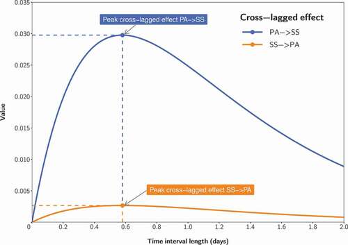
One characteristic of cross-lagged effects from cross-lagged panel models is that they depend on the time interval between measurement occasions. For different interval lengths, the cross-lagged effects differ in size. This is because the impact of a variable on another first needs to unfold before it reaches its maximum and then declines with the passing of more time. For instance, a high dose of physical activity stimulates biochemical processes in the body which results in strong muscle ache some time later with a peak effect after a certain time span (e.g., Hecht & Voelkle, 2021, determined such a time span to be around half a day). Then, after a couple of days, the impact of high physical activity from some days ago has dissipated. Thus, there is a roughly inverse-U-shaped curve that describes the size of a cross-lagged effect depending on the length of the time interval. Figure 1 (adapted from Hecht & Voelkle, 2021) illustrates such a curve. The values of the cross-lagged effects (y-axis) are plotted against the time interval length (x-axis). For a time interval of zero, the cross-lagged effect is, of course, zero because there cannot be an impact from one variable to another if no time has passed. When more time passes, the effect from physical activity on pain severity unfolds (the curve rises) and then reaches the maximum effect for a time interval of around half a day. For longer time intervals, the size of the cross-lagged effect (and the curve) declines toward zero again.

Figure 1. Discrete-time cross-lagged effects plot. PA = Physical activity; SS = Symptom severity. Adapted from Hecht and Voelkle (2021)

When researchers plan their longitudinal studies, they need to choose a specific length of the time interval between measurement occasions. This means that they obtain cross-lagged effects from cross-lagged panel analysis for this specific time interval. However, where these effects are located in the effect distribution across interval lengths and whether these effects are the peak effects is usually unknown and hardly explorable with cross-lagged panel models. A solution to this problem is continuous-time modeling which offers exactly this feature: the unfolding and dissipation of cross-lagged relations can be investigated, independently from the spacing of measurement occasions in the study design. This is made possible by conceptualizing humans as continuously existing entities and differential calculus.

Among psychologists, there is a rather broad consensus that the human system continuously exists at all points in time (within the time span of life). This understanding is, however, not fully utilized in cross-lagged panel models and other discrete-time models. In contrast, continuous-time modeling explicitly builds upon the continuous human nature. When we observe the continuously existing and evolving human system at certain discrete time points, we obtain “snapshots” that can be used to estimate the parameters that describe the continuous system dynamics which are represented by a stochastic differential equation (see, e.g., Oud & Delsing, 2010).

Unfortunately, the mathematics needed for continuous-time modeling are somewhat intricate (see, e.g., Voelkle et al., 2012, for a didactic introduction and Hecht et al., 2019, for examples and explanations on how to understand the mathematical model notation), but fortunately accessible software solutions like ctsem (Driver et al., 2017) exist for model estimation. Analogous to discrete-time models, the parameters that describe the continuous dynamics within the human system in continuous-time models are again effects that temporally relate one variable to itself (auto-effect) and to the other variables (cross-effects). To not confuse discrete-time cross-lagged modeling and continuous-time modeling, it is advisable to carefully distinguish parameter labels (an overview is given in the work of Hecht & Voelkle, 2021).

The mathematical relations between a continuous-time model and its corresponding time interval dependent discrete-time counterpart models are given by a set of equations (see, e.g., Equations 5–16(5) ${\omega }_{j(p-1)}\sim {\mathcal{N}}_F\left(\mathbf{0},{\mathbf{Q}}_{{\mathrm{\Delta }}_{p-1}}^{\ast }\right),$(5) in the Appendix of the work of Hecht & Voelkle, 2021, or Equations 6(6) ${\mathbf{A}}_{{\mathrm{\Delta }}_{p-1}}^{\ast }=exp(\mathbf{A}{\mathrm{\Delta }}_{p-1}),$(6) –8(8) $\mathrm{w}\mathrm{i}\mathrm{t}\mathrm{h}{\mathbf{A}}_{\mathrm{\#}}=\mathbf{A}\otimes {\mathbf{I}}_F+{\mathbf{I}}_F\otimes \mathbf{A}\mathrm{a}\mathrm{n}\mathrm{d}{\mathbf{Q}}_{\mathrm{\infty }}=\mathrm{i}\mathrm{r}\mathrm{o}\mathrm{w}\left(-{\mathbf{A}}_{\mathrm{\#}}^{-1}\mathrm{r}\mathrm{o}\mathrm{w}\mathbf{Q}\right)$(8) in this article further below). Hereby, a key feature is that the parameters of the one model that describes the continuously evolving human system (i.e., the continuous-time parameters) can be transformed into parameters of many discrete-time cross-lagged models that describe the dynamics for arbitrary time intervals between discrete points in time. This feature implies some of the advantages of continuous-time modeling: (1) The possibility to compute discrete-time parameters for any time interval allows for comparing results from studies which used different time intervals for the assessment. (2) Each person might be assessed at different points in time; data from such flexible longitudinal designs (Hecht et al., 2019) can be used to estimate the continuous-time parameters, because no matter when the assessments of persons were conducted, they all are snapshots of the same continuous phenomenon. (3) The unfolding and dissipation of effects can be studied and the time interval for which the interrelation between variables (i.e., the cross-lagged effects) is strongest can be determined.

Oftentimes, these peak effects are of central substantive interest and researchers want to conduct inferential statistical tests for them. Thus, the question of statistical power immediately arises. Especially in psychology with usually underpowered studies (Maxwell, 2004), statistical power has been and is a pivotal and much discussed topic, and researchers might welcome recommendations to achieve sufficient power.

Purpose and scope

In the present work, we identify a prediction model for statistical power of peak cross-lagged effects with continuous-time models and provide an easy-to-use Shiny App with which the statistical power can be roughly approximated. We assume that the statistical power of the peak cross-lagged effects in continuous-time models depends on the number of persons, the number of time points, and the size of the peak cross-lagged effect, because sample size and effect size are classic factors related to statistical power.

The article is organized into the following sections. First, we briefly present a popular continuous-time model which is suitable to explore peak cross-lagged effects, compare notations and parameterizations for this model, and cite some empirical applications of this model. Second, we report results from a simulation study in which we varied the number of persons, the number of time points, the effect size, and the size of the auto-effect, and then calculated the power for a null hypothesis test of the peak cross-lagged effect against zero ($\alpha =.05$). With the help of machine learning algorithms, we derive a prediction formula which could be used to roughly approximate power for study planning. Finally, we conclude with a discussion of our work (including limitations).

Multivariate continuous-time models

Model formulations

Continuous-time modeling is a popular approach in many disciplines, for instance, in the natural sciences, finance, and econometrics (e.g., Capasso & Bakstein, 2012; Dana & Jeanblanc, 2003; Gandolfo, 1993; Sinha & Rao, 1991). Recently, continuous-time modeling has found its way into the behavioral sciences (e.g., Van Montfort et al., 2018). Although continuous-time models come in various flavors, a common continuous-time model in the behavioral sciences and psychology is the linear stochastic differential equation model (Oud & Delsing, 2010), which may also be called continuous-time first-order vector autoregressive [CT-VAR(1)] model (Ryan et al., 2018), multivariate continuous-time model (Hecht & Voelkle, 2021), or multivariate Ornstein-Uhlenbeck process (e.g., Oravecz et al., 2018). The core of these models is a stochastic differential equation which can be conceptually written as:

(1) $\mathrm{d}\mathrm{e}\mathrm{r}\mathrm{i}\mathrm{v}\mathrm{a}\mathrm{t}\mathrm{i}\mathrm{v}\mathrm{e}=\mathrm{d}\mathrm{e}\mathrm{t}\mathrm{e}\mathrm{r}\mathrm{m}\mathrm{i}\mathrm{n}\mathrm{i}\mathrm{s}\mathrm{t}\mathrm{i}\mathrm{c}\mathrm{p}\mathrm{a}\mathrm{r}\mathrm{t}+\mathrm{s}\mathrm{t}\mathrm{o}\mathrm{c}\mathrm{h}\mathrm{a}\mathrm{s}\mathrm{t}\mathrm{i}\mathrm{c}\mathrm{p}\mathrm{a}\mathrm{r}\mathrm{t}.$(1)

The derivative is the result of performing a differentiation process upon a function which describes the state of the (human) system depending on time. Time is usually denoted with symbol $t$, whereas the notation of the vector which contains a value per variable (“state vector”) differs, for example, $\mathbf{x}$ (Oud & Delsing, 2010; Voelkle et al., 2012), $\mathbf{y}$ (Ryan et al., 2018), $\eta$ (Driver et al., 2017), $\mathbf{\Theta }$ (Oravecz et al., 2018), and $\theta$ (Hecht & Voelkle, 2021). The derivative is often given in Leibniz’s notation: $\frac{\mathrm{d}\mathbf{x}(t)}{\mathrm{d}t}$ (e.g., Oud & Delsing, 2010; Ryan et al., 2018; Voelkle et al., 2012). Some authors (e.g., Driver et al., 2017; Hecht & Voelkle, 2021; Oravecz et al., 2018) place the differential d$t$ on the right-hand side of the equation: $\mathrm{d}\mathbf{x}(t)=[\dots ]\mathrm{d}t$, presumably because the Wiener process is not differentiable (Singer, 2012).

The deterministic part contains the product of a matrix, which is usually referred to as the drift matrix, and the state vector. Many authors denote the drift matrix with the symbol $\mathbf{A}$, one exception being Oravecz et al.’s model where drift matrix $\mathbf{B}=-\mathbf{A}$. Further, a term relating to the mean levels of the processes is usually included. Often, either process intercepts, $\mathbf{b}$ (e.g., Driver et al., 2017; Oud & Delsing, 2010; Voelkle et al., 2012), or process means, $\mu$ (e.g., Oravecz et al., 2018; Ryan et al., 2018), are used. As the relation between process means and continuous-time intercepts is $\mu =-{\mathbf{A}}^{-1}\mathbf{b}$, these expressions are interchangeable, for example, $\mathbf{A}(\mathbf{x}-\mu )=\mathbf{A}\mathbf{x}+\mathbf{b}$.

The stochastic part comprises scaled derivatives or differentials of Wiener processes $\mathbf{W}(t)$ (i.e., random walks in continuous time) representing stochastic noise. The derivatives $\frac{\mathrm{d}\mathbf{W}(t)}{\mathrm{d}t}$ or differentials $\mathrm{d}\mathbf{W}(t)$ are scaled by the Cholesky factor of the covariance matrix of the noise. Oud et al. (2018) call this covariance matrix diffusion covariance matrix and its Cholesky factor diffusion matrix, whereas other authors (e.g., Oud & Delsing, 2010; Voelkle et al., 2012) call the covariance matrix “diffusion matrix” and impose no specific name on its Cholesky factor. Often, the covariance matrix is denoted with symbol $\mathbf{Q}$ and the Cholesky factor with $\mathbf{G}$, one exception being Oravecz et al.’s notation of $\mathrm{\Sigma }$ instead of $\mathbf{G}$.

Furthermore, continuous-time models frequently include a measurement part, for example, for continuous response data (e.g., Arminger, 1986; Chow et al., 2016; Deboeck & Boulton, 2016; Driver et al., 2017; Oud & Delsing, 2010; Oud & Jansen, 2000; Singer, 2012) or for dichotomous response data (Hecht et al., 2019). Also, various model extensions were proposed, for example, with individually varying continuous-time intercepts (e.g., Hecht & Voelkle, 2021; Oud & Delsing, 2010) and with time-independent and time-dependent predictors (e.g., Driver et al., 2017).

In summary, multivariate continuous-time models have been introduced to the behavioral and social sciences as exemplarily illustrated by the—not exhaustive—list of cited works above. The mathematical symbols, notations, parameterizations, names, and extensions might differ, but all the multivariate continuous-time models have the same stochastic differential equation core. Also, the popular continuous-time modeling software ctsem (Driver et al., 2017, 2020) is based on the multivariate continuous-time model and allows users to estimate this model.

Empirical applications

Multivariate continuous-time models (or their variants/extensions) have been applied in many areas of behavioral and social sciences research and other disciplines. Often, the number of processes under investigation was two, that is, a bivariate continuous-time model was employed. For example, Voelkle et al. (2012) illustrated the dynamic interplay of authoritarianism and anomia; Ryan et al. (2018) investigated the temporal relations between feeling down and being tired; Oravecz et al. (2018) showed how two core affect ratings, valence and arousal, are related across time; Tómasson (2018) illustrated the associations of temperature and CO₂ over 800,000 years; Crewther et al. (2020) studied the temporal relation of testosterone and motivation; Crewther et al. (2021) investigated the within-person coupling of testosterone and cortisol; Hecht and Voelkle (2021) illustrated the temporal associations between physical activity and pain; Mueller et al. (2018) estimated multiple bivariate continuous-time models to explore the bivariate dynamic relations between extraversion, neuroticism, physical functioning, and vision; Volz et al. (2019) investigated the dynamic interplay of general self-efficacy and post-stroke depression; Dormann et al. (2018) studied psychosocial safety climate and depression with the bivariate continuous-time model; and, to complete our exemplary non-exhaustive list of empirical applications, Ehm et al. (2019) examined the relation between academic self-concept and achievement.

Overall, continuous-time modeling has been applied in research practice. As the multivariate continuous-time model is a more general variant of the popular (random intercept) cross-lagged panel model [(RI)-CLPM; e.g., Hamaker et al., 2015; Kearney, 2017; Selig & Little, 2012] we are optimistic that the usage of multivariate continuous-time models will accelerate.

Model formulation in the current study

The formulation of the multivariate continuous-time model in the current study is largely based on the work of Oud and Delsing (2010) with slight notational adaptations. The core of our model is the standard stochastic differential equation as described above. In our notation it reads:

(2) $\frac{\mathrm{d}{\mathbf{y}}_{jt}}{\mathrm{d}t}=\mathbf{A}\left({\mathbf{y}}_{jt}-{\mu }_j\right)+\mathbf{G}\frac{\mathrm{d}{\mathbf{W}}_{jt}}{\mathrm{d}t},$(2)

where ${\mathbf{y}}_{jt}\in {\mathbb{R}}^F$ is the state vector of person $j$’s $F$-dimensional dynamical system at continuous time $t\in \mathbb{R}$ (with $F$ being the total number of variables or “processes”). $\frac{\mathrm{d}{\mathbf{y}}_{jt}}{\mathrm{d}t}$ is the derivative, which may be interpreted as the instantaneous rate of change (or velocity) of the system at time $t$. The $F\times F$ drift matrix $\mathbf{A}$ contains the auto-effects (on the main diagonal) and cross-effects (on the off-diagonals) and thus characterizes the temporal dynamics of the variables. In the present work, we limit our delineations to continuous-time models in which the real-parts of the eigenvalues of $\mathbf{A}$ are negative. The vector ${\mu }_j\in {\mathbb{R}}^F$ contains the individual means. Noise is represented by a multivariate Wiener process ${\mathbf{W}}_{jt}\in {\mathbb{R}}^F$ and $\frac{\mathrm{d}{\mathbf{W}}_{jt}}{\mathrm{d}t}$ is its formal derivative. The $F\times F$ diffusion covariance matrix $\mathbf{Q}={\mathbf{G}\mathbf{G}}^{\prime }$ is the covariance matrix of this noise, and $\mathbf{G}$ is the Cholesky factor of $\mathbf{Q}$ representing the effect of the noise.

The solution of the stochastic differential equation (Equation 2(2) $\frac{\mathrm{d}{\mathbf{y}}_{jt}}{\mathrm{d}t}=\mathbf{A}\left({\mathbf{y}}_{jt}-{\mu }_j\right)+\mathbf{G}\frac{\mathrm{d}{\mathbf{W}}_{jt}}{\mathrm{d}t},$(2) ) is given as:

(3) $\mathrm{f}\mathrm{o}\mathrm{r}p\ge 2,{\mathbf{y}}_{jp}={\mathbf{A}}_{{\mathrm{\Delta }}_{p-1}}^{\ast }{\mathbf{y}}_{j(p-1)}+\left({\mathbf{I}}_F-{\mathbf{A}}_{{\mathrm{\Delta }}_{p-1}}^{\ast }\right){\mu }_j+{\omega }_{j(p-1)},$(3)

(4) ${\mu }_j\sim {\mathcal{N}}_F\left(\mu ,{\mathrm{\Sigma }}_{\mathrm{\infty }}\right),$(4)

(5) ${\omega }_{j(p-1)}\sim {\mathcal{N}}_F\left(\mathbf{0},{\mathbf{Q}}_{{\mathrm{\Delta }}_{p-1}}^{\ast }\right),$(5)

(6) ${\mathbf{A}}_{{\mathrm{\Delta }}_{p-1}}^{\ast }=exp(\mathbf{A}{\mathrm{\Delta }}_{p-1}),$(6)

(7) ${\mathbf{Q}}_{{\mathrm{\Delta }}_{p-1}}^{\ast }=\mathrm{i}\mathrm{r}\mathrm{o}\mathrm{w}\left\{-\left[exp({\mathbf{A}}_{\mathrm{\#}}{\mathrm{\Delta }}_{p-1})-{\mathbf{I}}_{F^2}\right]\mathrm{r}\mathrm{o}\mathrm{w}{\mathbf{Q}}_{\mathrm{\infty }}\right\},$(7)

(8) $\mathrm{w}\mathrm{i}\mathrm{t}\mathrm{h}{\mathbf{A}}_{\mathrm{\#}}=\mathbf{A}\otimes {\mathbf{I}}_F+{\mathbf{I}}_F\otimes \mathbf{A}\mathrm{a}\mathrm{n}\mathrm{d}{\mathbf{Q}}_{\mathrm{\infty }}=\mathrm{i}\mathrm{r}\mathrm{o}\mathrm{w}\left(-{\mathbf{A}}_{\mathrm{\#}}^{-1}\mathrm{r}\mathrm{o}\mathrm{w}\mathbf{Q}\right)$(8)

(9) $\mathrm{a}\mathrm{n}\mathrm{d}\mathrm{f}\mathrm{o}\mathrm{r}p=1,{\mathbf{y}}_{j1}\sim {\mathcal{N}}_F\left({\mu }_j+{\mu }_{\mathrm{d}\mathrm{e}\mathrm{v}},{\mathrm{\Sigma }}_{\mathrm{f}\mathrm{w}}\right),$(9)

where ${\mathbf{I}}_F$ and ${\mathbf{I}}_{F^2}$ are identity matrices of size $F$ and $F^2$, respectively. $\otimes$ denotes the Kronecker product. The row operator puts the elements of a matrix row-wise in a column vector. The irow operator puts the elements from the column vector back into a matrix.

The interval dependent discrete-time part of the model is given by Equation 3(3) $\mathrm{f}\mathrm{o}\mathrm{r}p\ge 2,{\mathbf{y}}_{jp}={\mathbf{A}}_{{\mathrm{\Delta }}_{p-1}}^{\ast }{\mathbf{y}}_{j(p-1)}+\left({\mathbf{I}}_F-{\mathbf{A}}_{{\mathrm{\Delta }}_{p-1}}^{\ast }\right){\mu }_j+{\omega }_{j(p-1)},$(3) . Unequal-interval longitudinal designs usually involve responses of $j=1,\dots ,N$ persons at several points in time, $t_p$, with $p=1,\dots ,T$ being a running index denoting the discrete time point and $T$ being the number of time points. Time interval lengths ${\mathrm{\Delta }}_{p-1}$¹ between time points are given by ${\mathrm{\Delta }}_{p-1}=t_p-t_{p-1}$ for all $p\ge 2$. The values, $y_{jpf}$, of person $j$ at time point $p$ on variable $f=1,\dots ,F$ are stacked into the column vector ${\mathbf{y}}_{jp}$. This vector of each person at each time point is predicted by the matrix product of the autoregressive matrix² ${\mathbf{A}}_{{\mathrm{\Delta }}_{p-1}}^{\ast }$ and the vector ${\mathbf{y}}_{j(p-1)}$ of the person at the previous time point (which was ${\mathrm{\Delta }}_{p-1}$ time units ago) plus an intercept term (which is calculated from the individual mean) plus an error term ${\omega }_{j(p-1)}$. The individual means are assumed to be normally distributed with mean vector $\mu$ and covariance matrix ${\mathrm{\Sigma }}_{\mathrm{\infty }}$ (Equation 4(4) ${\mu }_j\sim {\mathcal{N}}_F\left(\mu ,{\mathrm{\Sigma }}_{\mathrm{\infty }}\right),$(4) ). The $\mathrm{\infty }$ symbol as subscript denotes “long-range” (or “asymptotic”, Driver et al., 2017) parameters that describe the system for $\mathrm{\Delta }$ $\to$ $\mathrm{\infty }$, that is, a system with no temporal relations (${\mathbf{A}}_{\mathrm{\Delta }\to \mathrm{\infty }}^{\ast }=\mathbf{0}$). The error term has a normal distribution with a zero vector as location and covariance matrix ${\mathbf{Q}}_{{\mathrm{\Delta }}_{p-1}}^{\ast }$ (Equation 5(5) ${\omega }_{j(p-1)}\sim {\mathcal{N}}_F\left(\mathbf{0},{\mathbf{Q}}_{{\mathrm{\Delta }}_{p-1}}^{\ast }\right),$(5) ). The interval-dependent discrete-time parameter matrices, ${\mathbf{A}}_{{\mathrm{\Delta }}_{p-1}}^{\ast }$ and ${\mathbf{Q}}_{{\mathrm{\Delta }}_{p-1}}^{\ast }$, are connected to the continuous-time drift matrix $\mathbf{A}$ via Equations 6(6) ${\mathbf{A}}_{{\mathrm{\Delta }}_{p-1}}^{\ast }=exp(\mathbf{A}{\mathrm{\Delta }}_{p-1}),$(6) –8(8) $\mathrm{w}\mathrm{i}\mathrm{t}\mathrm{h}{\mathbf{A}}_{\mathrm{\#}}=\mathbf{A}\otimes {\mathbf{I}}_F+{\mathbf{I}}_F\otimes \mathbf{A}\mathrm{a}\mathrm{n}\mathrm{d}{\mathbf{Q}}_{\mathrm{\infty }}=\mathrm{i}\mathrm{r}\mathrm{o}\mathrm{w}\left(-{\mathbf{A}}_{\mathrm{\#}}^{-1}\mathrm{r}\mathrm{o}\mathrm{w}\mathbf{Q}\right)$(8) . The interval-dependent error covariance matrix ${\mathbf{Q}}_{{\mathrm{\Delta }}_{p-1}}^{\ast }$ additionally depends on the within-person covariance matrix ${\mathbf{Q}}_{\mathrm{\infty }}$ (Equation 7(7) ${\mathbf{Q}}_{{\mathrm{\Delta }}_{p-1}}^{\ast }=\mathrm{i}\mathrm{r}\mathrm{o}\mathrm{w}\left\{-\left[exp({\mathbf{A}}_{\mathrm{\#}}{\mathrm{\Delta }}_{p-1})-{\mathbf{I}}_{F^2}\right]\mathrm{r}\mathrm{o}\mathrm{w}{\mathbf{Q}}_{\mathrm{\infty }}\right\},$(7) ), which is assumed equal across persons. For the first time point, the vector ${\mathbf{y}}_{j1}$ is normally distributed with the sum of the individual mean, ${\mu }_j$, and a deviation, ${\mu }_{\mathrm{d}\mathrm{e}\mathrm{v}}$, as location and a within-person covariance matrix ${\mathrm{\Sigma }}_{\mathrm{f}\mathrm{w}}$ (subscript “fw” stands for “first time point, within-person”). The to be estimated model parameters of this continuous-time model are the drift matrix $\mathbf{A}$, the covariance matrices ${\mathrm{\Sigma }}_{\mathrm{\infty }}$, ${\mathbf{Q}}_{\mathrm{\infty }}$, and ${\mathrm{\Sigma }}_{\mathrm{f}\mathrm{w}}$, and the mean vectors $\mu$ and ${\mu }_{\mathrm{d}\mathrm{e}\mathrm{v}}$.

The time interval dependent autoregressive matrix ${\mathbf{A}}_{{\mathrm{\Delta }}_{p-1}}^{\ast }$ (Equation 6(6) ${\mathbf{A}}_{{\mathrm{\Delta }}_{p-1}}^{\ast }=exp(\mathbf{A}{\mathrm{\Delta }}_{p-1}),$(6) ) contains the autoregressive effects (on the main diagonal) and the cross-lagged effects (on the off-diagonals):

${\mathbf{A}}_{{\mathrm{\Delta }}_{p-1}}^{\ast }=\left[\begin{array}{ccc}{a}_{{\mathrm{\Delta }}_{p-1},{\mathrm{Y}}_1}^{\ast }& \dots & a_{{\mathrm{\Delta }}_{p-1},{\mathrm{Y}}_F\to {\mathrm{Y}}_1}^{\ast }\\ ⋮& \ddots & ⋮\\ a_{{\mathrm{\Delta }}_{p-1},{\mathrm{Y}}_1\to {\mathrm{Y}}_F}^{\ast }& \dots & a_{{\mathrm{\Delta }}_{p-1},{\mathrm{Y}}_F}^{\ast }\end{array}\right].$

The autoregressive effects characterize the stability of the variables, that is, how predictive a value at one time point is for the value at the next time point. A high autoregressive effect indicates high stability/predictiveness, whereas a low autoregressive effect indicates low stability. A cross-lagged effect describes the prediction of one variable at a time point on another variable at the next time point. Cross-lagged effects may be interpreted like partial regression coefficients: A one unit change in the predictor variable is associated with an expected change of the dependent variable in the amount of the regression coefficient, holding the other predictors constant. For instance, a one unit change in ${\mathrm{Y}}_1$ would be associated with an expected change in ${\mathrm{Y}}_F$ in the amount of $a_{{\mathrm{\Delta }}_{p-1},{\mathrm{Y}}_1\to {\mathrm{Y}}_F}^{\ast }$ $\mathrm{\Delta }$ time units later when all other predictors are held constant.

For better comparability, the cross-lagged effects may be standardized with respect to the within-person variances, for example:

(10) $a_{{\mathrm{\Delta }}_{p-1},\mathrm{s}\mathrm{t}\mathrm{d},{\mathrm{Y}}_1\to {\mathrm{Y}}_F}^{\ast }=a_{{\mathrm{\Delta }}_{p-1},{\mathrm{Y}}_1\to {\mathrm{Y}}_F}^{\ast }\frac{\sqrt{{\sigma }_{\mathrm{w}{\mathrm{Y}}_1}^2}}{\sqrt{{\sigma }_{\mathrm{w}{\mathrm{Y}}_{\mathrm{F}}}^2}},$(10)

where ${\sigma }_{\mathrm{w}{\mathrm{Y}}_1}^2$ and ${\sigma }_{\mathrm{w}{\mathrm{Y}}_{\mathrm{F}}}^2$ are main diagonal elements from the within-person covariance matrix ${\mathbf{Q}}_{\mathrm{\infty }}$. The interpretation of standardized cross-lagged effects is similar to (non-standardized) cross-lagged effects, except that the units of both variables are now standard deviations. Thus, a standardized cross-lagged effect indicates the expected change of a variable ${\mathrm{Y}}_F$ at time $t$+$\mathrm{\Delta }$ in $S{D}_{{\mathrm{Y}}_F}$ units associated with a one $S{D}_{{\mathrm{Y}}_1}$ change of ${\mathrm{Y}}_1$ at time $t$ holding the other predictor variables constant.

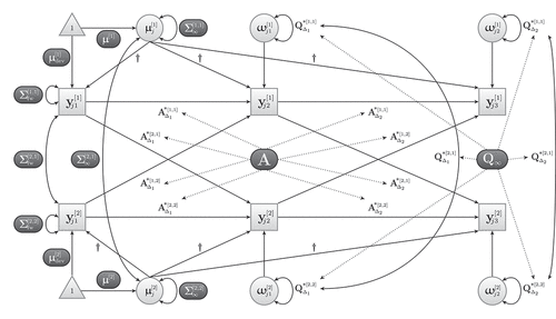
Figure 2 illustrates a bivariate continuous-time model for three time points. For more explanations, examples, and illustrations of this (and other) continuous-time models see, for instance, Voelkle et al. (2012), Driver et al. (2017), Hecht and Voelkle (2021), Hecht et al. (2019), Hecht and Zitzmann (2020), and Hecht and Zitzmann (2021).

Figure 2. The bivariate continuous-time model with three time points (schematic). Model parameters that are estimated are set in light text color on dark background. Dotted lines indicate parameter relations according to Equations 6(6) ${\mathbf{A}}_{{\mathrm{\Delta }}_{p-1}}^{\ast }=exp(\mathbf{A}{\mathrm{\Delta }}_{p-1}),$(6) and 7(7) ${\mathbf{Q}}_{{\mathrm{\Delta }}_{p-1}}^{\ast }=\mathrm{i}\mathrm{r}\mathrm{o}\mathrm{w}\left\{-\left[exp({\mathbf{A}}_{\mathrm{\#}}{\mathrm{\Delta }}_{p-1})-{\mathbf{I}}_{F^2}\right]\mathrm{r}\mathrm{o}\mathrm{w}{\mathbf{Q}}_{\mathrm{\infty }}\right\},$(7) . The dagger symbol $†$ indicates path coefficients derived from $\left({\mathbf{I}}_F-{\mathbf{A}}_{{\mathrm{\Delta }}_{p-1}}^{\ast }\right)$ in Equation 3(3) $\mathrm{f}\mathrm{o}\mathrm{r}p\ge 2,{\mathbf{y}}_{jp}={\mathbf{A}}_{{\mathrm{\Delta }}_{p-1}}^{\ast }{\mathbf{y}}_{j(p-1)}+\left({\mathbf{I}}_F-{\mathbf{A}}_{{\mathrm{\Delta }}_{p-1}}^{\ast }\right){\mu }_j+{\omega }_{j(p-1)},$(3)

Simulation study

Data generation

The data-generating model was the continuous-time model described in Equations 2(2) $\frac{\mathrm{d}{\mathbf{y}}_{jt}}{\mathrm{d}t}=\mathbf{A}\left({\mathbf{y}}_{jt}-{\mu }_j\right)+\mathbf{G}\frac{\mathrm{d}{\mathbf{W}}_{jt}}{\mathrm{d}t},$(2) –9(9) $\mathrm{a}\mathrm{n}\mathrm{d}\mathrm{f}\mathrm{o}\mathrm{r}p=1,{\mathbf{y}}_{j1}\sim {\mathcal{N}}_F\left({\mu }_j+{\mu }_{\mathrm{d}\mathrm{e}\mathrm{v}},{\mathrm{\Sigma }}_{\mathrm{f}\mathrm{w}}\right),$(9) with $F=2$ processes (i.e., a bivariate continuous-time model). The non-varied true model parameters were:

${\mathrm{\Sigma }}_{\mathrm{\infty }}={\mathbf{Q}}_{\mathrm{\infty }}={\mathrm{\Sigma }}_{\mathrm{f}\mathrm{w}}=\left[\begin{array}{cc}1& 0\\ 0& 1\end{array}\right]\mathrm{a}\mathrm{n}\mathrm{d}{\mu }_{\mathrm{\infty }}={\mu }_{\mathrm{d}\mathrm{e}\mathrm{v}}=\left[\begin{array}{c}0\\ 0\end{array}\right].$

The drift matrix $\mathbf{A}$ contains the auto-effects $a_{11}$ and $a_{22}$, which were varied in the simulation design, on the main diagonal and the cross-effects $a_{21}$ and $a_{12}$ as off-diagonal elements, which were determined from the varied peak standardized cross-lagged effects, $a_{\mathrm{p}\mathrm{e}\mathrm{a}\mathrm{k},\mathrm{s}\mathrm{t}\mathrm{d},{\mathrm{Y}}_1\to {\mathrm{Y}}_2}^{\ast }$ and $a_{\mathrm{p}\mathrm{e}\mathrm{a}\mathrm{k},\mathrm{s}\mathrm{t}\mathrm{d},{\mathrm{Y}}_2\to {\mathrm{Y}}_1}^{\ast }$, and the other model parameters. Inserting the true parameter values into the model equations (Equations 3(3) $\mathrm{f}\mathrm{o}\mathrm{r}p\ge 2,{\mathbf{y}}_{jp}={\mathbf{A}}_{{\mathrm{\Delta }}_{p-1}}^{\ast }{\mathbf{y}}_{j(p-1)}+\left({\mathbf{I}}_F-{\mathbf{A}}_{{\mathrm{\Delta }}_{p-1}}^{\ast }\right){\mu }_j+{\omega }_{j(p-1)},$(3) –9(9) $\mathrm{a}\mathrm{n}\mathrm{d}\mathrm{f}\mathrm{o}\mathrm{r}p=1,{\mathbf{y}}_{j1}\sim {\mathcal{N}}_F\left({\mu }_j+{\mu }_{\mathrm{d}\mathrm{e}\mathrm{v}},{\mathrm{\Sigma }}_{\mathrm{f}\mathrm{w}}\right),$(9) ) gives the data-generating model:

${\mu }_{j\mathrm{\infty }}\sim {\mathcal{N}}_2\left(\left[\begin{array}{c}0\\ 0\end{array}\right],\left[\begin{array}{cc}1& 0\\ 0& 1\end{array}\right]\right);$

$\mathrm{f}\mathrm{o}\mathrm{r}p=1,{\mathbf{y}}_{j1}\sim {\mathcal{N}}_2\left({\mu }_{j\mathrm{\infty }}+\left[\begin{array}{c}0\\ 0\end{array}\right],\left[\begin{array}{cc}1& 0\\ 0& 1\end{array}\right]\right);$

$\mathrm{f}\mathrm{o}\mathrm{r}p\ge 2,{\mathrm{\Delta }}_{p-1}\sim {\mathcal{U}}_{\{0.20,0.40,0.60,0.80\}},$

${\mathbf{A}}_{{\mathrm{\Delta }}_{p-1}}^{\ast }=exp\left(\left[\begin{array}{cc}{a}_{11}& a_{12}\\ a_{21}& a_{22}\end{array}\right]{\mathrm{\Delta }}_{p-1}\right),$

${\mathbf{Q}}_{{\mathrm{\Delta }}_{p-1}}^{\ast }=\mathrm{i}\mathrm{r}\mathrm{o}\mathrm{w}\left\{-\left\{exp\left\{\left[\begin{array}{cccc}2a_{11}& a_{12}& a_{12}& 0\\ a_{21}& a_{22}+a_{11}& 0& a_{12}\\ a_{21}& 0& a_{22}+a_{11}& a_{12}\\ 0& a_{21}& a_{21}& 2a_{22}\end{array}\right]{\mathrm{\Delta }}_{p-1}\right\}-{\mathbf{I}}_4\right\}\left[\begin{array}{c}1\\ 0\\ 0\\ 1\end{array}\right]\right\},$

${\omega }_{j(p-1)}\sim {\mathcal{N}}_2\left(\left[\begin{array}{c}0\\ 0\end{array}\right],{\mathbf{Q}}_{{\mathrm{\Delta }}_{p-1}}^{\ast }\right),$

${\mathbf{y}}_{jp}={\mathbf{A}}_{{\mathrm{\Delta }}_{p-1}}^{\ast }{\mathbf{y}}_{j(p-1)}+\left({\mathbf{I}}_2-{\mathbf{A}}_{{\mathrm{\Delta }}_{p-1}}^{\ast }\right){\mu }_{j\mathrm{\infty }}+{\omega }_{j(p-1)},$

where ${\mathcal{N}}_2$ denotes a bivariate normal and $\mathcal{U}$ a uniform distribution, and ${\mathbf{I}}_2$ and ${\mathbf{I}}_4$ are identity matrices of size 2 and 4, respectively. Please note that ${\mathrm{\Delta }}_{p-1}$ is constant across persons which is a characteristic of an “unequal-interval nonindividualized design” (Hecht et al., 2019) and that the intra-class correlation is 0.50.

Simulation design

We varied the following factors in our simulation study: number of persons ($N$ = 5, 10, 20, 30, 40, 50, or 60), number of time points ($T$ = 5, 10, 20, 30, 40, 50, or 60), size of the peak standardized cross-lagged effect from process 1 to process 2 ($a_{\mathrm{p}\mathrm{e}\mathrm{a}\mathrm{k},\mathrm{s}\mathrm{t}\mathrm{d},{\mathrm{Y}}_1\to {\mathrm{Y}}_2}^{\ast }$ = $-0.15$, $-0.10$, $-0.05$, 0.05, 0.10, 0.15), size of the peak standardized cross-lagged effect from process 2 to process 1 ($a_{\mathrm{p}\mathrm{e}\mathrm{a}\mathrm{k},\mathrm{s}\mathrm{t}\mathrm{d},{\mathrm{Y}}_2\to {\mathrm{Y}}_1}^{\ast }$ = $-0.15$, $-0.10$, $-0.05$, 0.05, 0.10, 0.15), auto-effect of process 1 ($a_{11}$ = $-1.05$, $-0.70$, $-0.45$), and auto-effect of process 2 ($a_{22}$ = $-1.05$, $-0.70$, $-0.45$). Throughout this work, cross-lagged parameters were standardized using the within-person variances (see Equation 10)(10) $a_{{\mathrm{\Delta }}_{p-1},\mathrm{s}\mathrm{t}\mathrm{d},{\mathrm{Y}}_1\to {\mathrm{Y}}_F}^{\ast }=a_{{\mathrm{\Delta }}_{p-1},{\mathrm{Y}}_1\to {\mathrm{Y}}_F}^{\ast }\frac{\sqrt{{\sigma }_{\mathrm{w}{\mathrm{Y}}_1}^2}}{\sqrt{{\sigma }_{\mathrm{w}{\mathrm{Y}}_{\mathrm{F}}}^2}},$(10) . To keep the simulation design within manageable and sensible boundaries, we did not fully cross all factors. The auto-effects of process 1 and 2 were paired: $-1.05$/$-1.05$, $-0.70$/$-0.70$, and $-0.45$/$-0.45$. The peak effect sizes were completely crossed and these pairs were completely crossed with the auto-effect pairs. To avoid uninformative power estimates of (or very close to) zero or one, combinations of smaller effects (all combinations that include absolute effect sizes of 0.05) were combined with the fully crossed subsets of $N$ = 30, …, 60 and $T$ = 30, …, 60, whereas combinations of higher effects (all combinations that include absolute effect sizes of 0.10 and 0.15) were combined with the fully crossed subsets of $N$ = 5, …, 30 and $T$ = 5, …, 30. All other effect size combinations (absolute effect combinations of 0.05/0.10 and 0.05/0.15) were combined with the fully crossed $N$ and $T$. This procedure resulted in a total of 3,312 design cells. A detailed overview of the simulation design is provided in the supplementary material.

Analysis

We randomly drew cells from the design, generated data sets, and ran models until the available CPU time of 1,650 days was exploited. The mean number of replications per design cell was $M_{N_{\mathrm{r}\mathrm{e}\mathrm{p}\mathrm{l}}}=574$ (min = 378, max = 802), the mean convergence rate was $M_{\mathrm{c}\mathrm{o}\mathrm{n}\mathrm{v}\mathrm{r}\mathrm{a}\mathrm{t}\mathrm{e}}=0.81$ (min = 0.30, max = 1.00), and the mean number of converged models was $M_{N\mathrm{c}\mathrm{o}\mathrm{n}\mathrm{v}\mathrm{e}\mathrm{r}\mathrm{g}\mathrm{e}\mathrm{d}}=462$ (min = 153, max = 652). All models were estimated using the maximum likelihood estimator of the R package ctsem (R Core Team, 2020; Driver et al., 2020) which interfaces to OpenMx (Neale et al., 2016) and each model ran on one Intel Xeon Gold 5120 (2.20 GHz) CPU of a 64-bit Linux Debian 10 “Buster” computer. A model was considered as converged if the OpenMx exit code was 0 and the standard errors of all parameters were unflawed (i.e., if they were non-missing and below 1,000). The analysis model was identical with the data-generating model. For each replication, the peak standardized cross-lagged effect was deemed insignificant (coded as 0) when its 95% confidence interval (CI) covered the value 0 and significant (coded as 1) when 0 was not covered by the confidence interval. The 95% CI for an undirected alternative hypothesis (population value $\ne$ 0) was calculated as: parameter $\pm$ 1.96 $\cdot$ $SE$ (Voelkle et al., 2012), with $SE$ being the standard error of the parameter.

We used machine learning techniques to derive a prediction model for the power of the peak standardized cross-lagged effects. Specifically, we combined $k$-fold cross validation (e.g., Kuhn & Johnson, 2013) with stepwise logistic regression. The number of folds was $k=10$ and thus, there were ten training sets (each comprised of nine folds) and ten corresponding test sets (one fold). The folds were created with function createMultiFolds() from R package caret (Kuhn et al., 2020). Within each replicate of the cross-validation, a stepwise logistic regression was conducted with function stepAIC() from the R package MASS (Ripley et al., 2021). The dependent variable was the dichotomous significance of the peak standardized cross-lagged effect. The stepwise regression algorithm started with the intercept-only model; the potentially maximal model included the intercept, the number of persons $N$, the number of time points $T$, the estimated peak standardized cross-lagged effect, the estimated absolute peak standardized cross-lagged effect, two-way interactions of these terms, and quadratic and cubic polynomials of these terms. The direction of the selection algorithm was both forward and backward and the criterion was AIC. As results of this machine learning approach, we report the differences concerning the selected predictors and statistics of AIC between training sets and prediction accuracy statistics (calculated with function confusionMatrix() from R package caret) when using the trained prediction model for the test set data. The final model is then estimated from the entire data with the identified relevant predictors.

Results

All ten stepwise logistic regression models resulted in the same selected parameters. AICs were very comparable with practically no variation between training sets ($M_{\mathrm{A}\mathrm{I}\mathrm{C}}=14,581,609$, $\mathrm{m}\mathrm{i}{\mathrm{n}}_{\mathrm{A}\mathrm{I}\mathrm{C}}=14,580,228$, $\mathrm{m}\mathrm{a}{\mathrm{x}}_{\mathrm{A}\mathrm{I}\mathrm{C}}=14,582,725$, $S{D}_{\mathrm{A}\mathrm{I}\mathrm{C}}=808$). The prediction accuracies based on the test sets were very comparable and high with $M_{\mathrm{a}\mathrm{c}\mathrm{c}}=0.8854$, $\mathrm{m}\mathrm{i}{\mathrm{n}}_{\mathrm{a}\mathrm{c}\mathrm{c}}=0.8853$, $\mathrm{m}\mathrm{a}{\mathrm{x}}_{\mathrm{a}\mathrm{c}\mathrm{c}}=0.8855$, $S{D}_{\mathrm{a}\mathrm{c}\mathrm{c}}<0.0001$. This may be interpreted as an indication that the data might not be overfitted. The estimates of the final model are given in Table 1.

Table 1. Parameter estimates from the logistic regression model for the prediction of statistical power of peak cross-lagged effects

Parameter	Value
Intercept	−11.47
$N$	0.37
$T$	0.14
$a_{\mathrm{s}\mathrm{t}\mathrm{d},\mathrm{p}\mathrm{e}\mathrm{a}\mathrm{k}}^{\ast }$	−0.33
$\left|a_{\mathrm{s}\mathrm{t}\mathrm{d},\mathrm{p}\mathrm{e}\mathrm{a}\mathrm{k}}^{\ast }\right|$	20.67
$N^2$	−0.0092
$T^2$	−0.0042
$a_{\mathrm{s}\mathrm{t}\mathrm{d},\mathrm{p}\mathrm{e}\mathrm{a}\mathrm{k}}^{\ast 2}$	−36.41
$N^3$	0.000071
$T^3$	0.000030
${|a{ }_{\mathrm{s}\mathrm{t}\mathrm{d},\mathrm{p}\mathrm{e}\mathrm{a}\mathrm{k}}^{\ast }|}^3$	10.80
$N\times T$	0.0014
$N\times a_{\mathrm{s}\mathrm{t}\mathrm{d},\mathrm{p}\mathrm{e}\mathrm{a}\mathrm{k}}^{\ast }$	0.0024
$N\times |a_{\mathrm{s}\mathrm{t}\mathrm{d},\mathrm{p}\mathrm{e}\mathrm{a}\mathrm{k}}^{\ast }|$	0.12
$T\times |a_{\mathrm{s}\mathrm{t}\mathrm{d},\mathrm{p}\mathrm{e}\mathrm{a}\mathrm{k}}^{\ast }|$	1.04
$a_{\mathrm{s}\mathrm{t}\mathrm{d},\mathrm{p}\mathrm{e}\mathrm{a}\mathrm{k}}^{\ast }\times |a_{\mathrm{s}\mathrm{t}\mathrm{d},\mathrm{p}\mathrm{e}\mathrm{a}\mathrm{k}}^{\ast }|$	0.47

$N$: Number of persons; $T$: Number of time points; $a_{\mathrm{s}\mathrm{t}\mathrm{d},\mathrm{p}\mathrm{e}\mathrm{a}\mathrm{k}}^{\ast }$: Value of peak

standardized cross-lagged effect.

Recommendations and Shiny App

Our general recommendation to determine power for a specific study design and analysis approach is, of course, to either calculate the power with analytically derived equations or – if no analytical solutions exist – to conduct tailored simulation studies. Such simulations, however, can become complex and cumbersome. Then instead, our prediction model might be used to obtain a rough power estimate (although we acknowledge that generalizing our findings beyond the studied conditions is arguable and limitations apply, see Discussion).

Based on our results (final model estimates in Table 1), we programed a Shiny App (available at https://psychtools.shinyapps.io/ContinuousTimePowerCalculation) for power calculations of peak standardized cross-lagged effects. Inputs are the number of persons $N$, the number of time points $T$, and the targeted value of the peak standardized cross-lagged effect. The output is the power of the peak standardized effect for $\alpha =0.05$ and an undirected alternative hypothesis that the effect is unequal zero.

Discussion

One of the strengths of continuous-time (vs. discrete-time) modeling is the facilitation of exploring the unfolding and dissipation of dynamic effects by deriving discrete-time cross-lagged effects for a variety of time interval lengths from the estimated continuous-time model parameters and then determining the peak effect. Plotting the values of the cross-lagged effects against their time interval lengths can provide visual support for exploring the shape of the cross-lagged effect distribution. This feature of continuous-time models might be advantageous for study planning as well. The interval length between measurement occasions can be flexibilized (to some degree), because the cross-lagged relations can be explored independently from the spacing of measurement occasions in the study design.

Researchers might be interested in the peak cross-lagged effects as these characterize the maximal impact from one variable on another. Thus, for study planning, the statistical power to detect those peak cross-lagged effects might be of interest. Analytically derived formulas or tailored simulation studies could be used for power calculations. However, to our best knowledge, such analytical solutions do not exist or are not publicly available. This leaves researchers with the option to conduct simulation studies, which are, however, challenging. To give some rough guidance, we conducted a simulation study and derived a prediction formula using machine learning techniques.

Generalizability of the results is limited to the conditions that were studied. Due to limited computational resources, it was not possible to investigate all potentially relevant factors and the extent of variation of the included factors, the degree of factor crossings, and the number of replications was limited. We rather heavily varied and crossed number of persons, number of time points, and effect size, as these factors were expected to be very predictive. However, the auto-effect entered the simulation study with only three different values, and both auto-effects had the same value in each design cell. We varied only the auto-effect, but not the other model parameters, and the intra-class correlation was constant as well. We used a bivariate continuous-time model (two variables) with individual means for which a normal distribution was assumed. Significance was determined with confidence intervals based on the assumption of normal parameter distributions. The assessment design was unequally spaced (different interval lengths between measurement occasions) but the same for each person. Only one software/estimation method was employed. Thus, our results might not generalize to other conditions, particularly not to settings where auto-effects are much larger, where the auto-effects of the processes differ in size, where the other model parameters exhibit other values, to continuous-time models with more than two variables and other assumptions about individual parameters, to other intra-class correlations, to different procedures for determining significance, to different assessment designs (e.g., individualized designs), to other software and estimation method. The employed model was a bivariate continuous-time model with random intercepts (which is a more general variant of the bivariate random intercepts cross-lagged panel model, RI-CLPM). Generalizability to other models is limited.

One limitation of the bivariate continuous-time model is that both discrete-time cross-lagged effects have their maxima for the same interval length. Researchers should be aware of this limitation and avoid the use of bivariate continuous-time models when this restriction is not theoretically supported.

The dependent variable in the present study was statistical power. For study planning, other criteria might be of interest as well. For instance, Hecht and Zitzmann (2021) illustrated the dependence of model performance (an aggregated measure consisting of convergence, bias, and coverage) on number of persons $N$ and time points $T$. So even if a sufficient statistical power is achieved with some $N$ and $T$, model performance might still be suboptimal.

Further limitations are that our results are based on a rather small amount of data (due to restricted computational resources), that we conducted our power analyses only for the very common significance level $\alpha =.05$ and an undirected alternative hypothesis, that the regression model might not contain all relevant factors and does not perfectly predict power, and that our analysis model was identical to the data-generating model. Negative effects of model misspecifications on estimation performance in autoregressive modeling contexts have been shown, for example, by Tanaka and Maekawa (1984) and Kunitomo and Yamamoto (1985); thus, negative effects of model misspecifications on power are imaginable as well. Further, the peak cross-lagged effects might be located in regions with no or sparse data and the quality of such interpolations might also depend on design characteristics.

In sum, this leaves enough material for future research on statistical power in continuous-time modeling which we consider quite worthwhile because we believe that continuous-time modeling will become even more prominent fueled by the rise of intensive longitudinal methods like the experience sampling method (ESM), ecological momentary assessment (EMA), and ambulatory assessment (AA). In future research, it would be interesting to derive analytical solutions to avoid the discussed limitations concerning generalizability. Until then, our prediction model may be used as a preliminary bridging approach. In this regard, we see our article as one step forward toward a full understanding of statistical power in continuous-time modeling.

In light of the limitations, we caution to use our presented results unreflectingly. Still, we think that we made a modest contribution and hope that researchers who are interested in exploring the unfolding of dynamic effects will find the results and recommendations useful.

Additional information

Funding

We acknowledge support by the Open Access Publication Fund of Humboldt-Universität zu Berlin.

Notes

¹ As ${\mathrm{\Delta }}_{p-1}$ is constant across persons, the design may be called “unequal-interval nonindividualized” (Hecht et al., 2019).

² In line with Oud and Delsing (2010) we use the asterisk symbol * to denote discrete-time parameters that can be calculated from continuous-time parameters.

References

- Arminger, G. (1986). Linear stochastic differential equation models for panel data with unobserved variables. Sociological Methodology, 16, 187–212. https://doi.org/10.2307/270923
- Bentler, P. M. (1980). Multivariate analysis with latent variables: Causal modeling. Annual Review of Psychology, 31, 419–456. https://doi.org/10.1146/annurev.ps.31.020180.002223
- Bollen, K. A., & Curran, P. J. (2006). Latent curve models: A structural equation perspective. Wiley-Interscience.
- Capasso, V., & Bakstein, D. (2012). An introduction to continuous-time stochastic processes: Theory, models, and applications to finance, biology, and medicine. Birkhäuser. https://doi.org/10.1007/978-0-8176-8346-7
- Chow, S.-M., Lu, Z., Sherwood, A., & Zhu, H. (2016). Fitting nonlinear ordinary differential equation models with random effects and unknown initial conditions using the stochastic approximation expectation–maximization (SAEM) algorithm. Psychometrika, 81, 102–134. https://doi.org/10.1007/s11336-014-9431-z
- Crewther, B. T., Hecht, M., & Cook, C. J. (2021). Diurnal within-person coupling between testosterone and cortisol in healthy men: Evidence of positive and bidirectional time-lagged associations using a continuous-time model. Adaptive Human Behavior and Physiology. Advance online publication. http://dx.doi.org/10.1007/s40750-021-00162-8
- Crewther, B. T., Hecht, M., Potts, N., Kilduff, L. P., Drawer, S., Marshall, E., & Cook, C. J. (2020). A longitudinal investigation of bidirectional and time-dependent interrelationships between testosterone and training motivation in an elite rugby environment. Hormones and Behavior, 126, 1–8. http://doi.org/10.1016/j.yhbeh.2020.104866
- Dana, R.-A., & Jeanblanc, M. (2003). Financial markets in continuous time. Springer. https://doi.org/10.1007/978-3-540-71150-6
- Deboeck, P. R., & Boulton, A. J. (2016). Integration of stochastic differential equations using structural equation modeling: A method to facilitate model fitting and pedagogy. Structural Equation Modeling, 23, 888–903. https://doi.org/10.1080/10705511.2016.1218763
- Dormann, C., Owen, M., Dollard, M., & Guthier, C. (2018). Translating cross-lagged effects into incidence rates and risk ratios: The case of psychosocial safety climate and depression. Work & Stress, 32, 248–261. https://doi.org/10.1080/02678373.2017.1395926
- Driver, C. C., Oud, J. H. L., & Voelkle, M. C. (2017). Continuous time structural equation modeling with R package ctsem. Journal of Statistical Software, 77. 1–35. https://doi.org/10.18637/jss.v077.i05
- Driver, C. C., Oud, J. H. L., & Voelkle, M. C. (2020). ctsem: Continuous time structural equation modelling (Version 3.2.1) [Computer software]. https://cran.r-project.org/package=ctsem
- Ehm, J.-H., Hasselhorn, M., & Schmiedek, F. (2019). Analyzing the developmental relation of academic self-concept and achievement in elementary school children: Alternative models point to different results. Developmental Psychology, 55, 2336–2351. https://doi.org/10.1037/dev0000796
- Gandolfo, G. (Ed.). (1993). Continuous-time econometrics. Springer. https://doi.org/10.1007/978-94-011-1542-1
- Greenberg, D. F., & Kessler, R. C. (1982). Equilibrium and identification in linear panel models. Sociological Methods & Research, 10, 435–451. https://doi.org/10.1177/0049124182010004003
- Hamaker, E. L., Kuiper, R. M., & Grasman, R. P. P. P. (2015). A critique of the cross-lagged panel model. Psychological Methods, 20, 102–116. https://doi.org/10.1037/a0038889
- Hecht, M., Hardt, K., Driver, C. C., & Voelkle, M. C. (2019). Bayesian continuous-time Rasch models. Psychological Methods, 24, 516–537. https://doi.org/10.1037/met0000205
- Hecht, M., & Voelkle, M. C. (2021). Continuous-time modeling in prevention research: An illustration. International Journal of Behavioral Development, 45, 19–27. https://doi.org/10.1177/0165025419885026
- Hecht, M., & Zitzmann, S. (2020). A computationally more efficient Bayesian approach for estimating continuous-time models. Structural Equation Modeling: A Multidisciplinary Journal, 27, 829–840. https://doi.org/10.1080/10705511.2020.1719107
- Hecht, M., & Zitzmann, S. (2021). Sample size recommendations for continuous-time models: Compensating shorter time-series with higher numbers of persons and vice versa. Structural Equation Modeling: A Multidisciplinary Journal 28, 229–236. https://doi.org/10.1080/10705511.2020.1779069
- Kearney, M. W. (2017). Cross-lagged panel analysis. In M. Allen (Ed.), The SAGE encyclopedia of communication research methods (pp. 313–314). SAGE. https://doi.org/10.4135/9781483381411.n117
- Kuhn, M., & Johnson, K. (2013). Applied predictive modeling. Springer. https://doi.org/10.1007/978-1-4614-6849-3
- Kuhn, M., Wing, J., Weston, S., Williams, A., Keefer, C., Engelhardt, A., Cooper, T., Mayer, Z., Kenkel, B., R Core Team, Benesty, M., Lescarbeau, R., Ziem, A., Scrucca, L., Tang, Y., Candan, C., & Hunt, T. (2020). caret: Classification and regression training (Version 6.0-86) [Computer software]. https://CRAN.R-project.org/package=caret
- Kunitomo, N., & Yamamoto, T. (1985). Properties of predictors in misspecified autoregressive time series models. Journal of the American Statistical Association, 80, 941–950. https://doi.org/10.1080/01621459.1985.10478208
- Maxwell, S. E. (2004). The persistence of underpowered studies in psychological research: Causes, consequences, and remedies. Psychological Methods, 9, 147–163. https://doi.org/10.1037/1082-989X.9.2.147
- Mayer, L. S. (1986). On cross-lagged panel models with serially correlated errors. Journal of Business & Economic Statistics, 4, 347–357. https://doi.org/10.1080/07350015.1986.10509531
- Mueller, S., Wagner, J., Smith, J., Voelkle, M. C., & Gerstorf, D. (2018). The interplay of personality and functional health in old and very old age: Dynamic within-person interrelations across up to 13 years. Journal of Personality and Social Psychology, 115, 1127–1147. https://doi.org/10.1037/pspp0000173
- Neale, M. C., Hunter, M. D., Pritikin, J. N., Zahery, M., Brick, T. R., Kirkpatrick, R. M., Estabrook, R., Bates, T. C., Maes, H. H., & Boker, S. M. (2016). OpenMx 2.0: Extended structural equation and statistical modeling. Psychometrika, 81, 535–549. https://doi.org/10.1007/s11336-014-9435-8
- Oravecz, Z., Wood, J., & Ram, N. (2018). On fitting a continuous-time stochastic process model in the Bayesian framework. In K. Van Montfort, J. H. L. Oud, & M. C. Voelkle (Eds.), Continuous time modeling in the behavioral and related sciences (pp. 55–78). Springer International. https://doi.org/10.1007/978-3-319-77219-6_3
- Oud, J. H. L., & Delsing, M. J. M. H. (2010). Continuous time modeling of panel data by means of SEM. In K. Van Montfort, J. H. L. Oud, & A. Satorra (Eds.), Longitudinal research with latent variables (pp. 201–244). Springer.
- Oud, J. H. L., Voelkle, M. C., & Driver, C. C. (2018). First- and higher-order continuous time models for arbitrary N using SEM. In K. Van Montfort, J. H. L. Oud, & M. C. Voelkle (Eds.), Continuous time modeling in the behavioral and related sciences (pp. 1–26). Springer International. https://doi.org/10.1007/978-3-319-77219-6
- Oud, J. H. L., & Jansen, R. A. R. G. (2000). Continuous time state space modeling of panel data by means of SEM. Psychometrika, 65, 199–215. https://doi.org/10.1007/BF02294374
- R Core Team (2020). R: A language and environment for statistical computing (Version 4.0.0) [Computer software]. R Foundation for Statistical Computing. https://www.r-project.org
- Ripley, B., Venables, B., Bates, D. M., Hornik, K., Gebhardt, A., & Firth, D. (2021). MASS: Support functions and datasets for venables and Ripley’s MASS (Version 7.3-53.1) [Computer software]. https://CRAN.R-project.org/package=MASS
- Ryan, O., Kuiper, R. M., & Hamaker, E. L. (2018). A continuous time approach to intensive longitudinal data: What, why and how? In K. Van Montfort, J. H. L. Oud, & M. C. Voelkle (Eds.), Continuous time modeling in the behavioral and related sciences (pp. 27–57). Springer International. https://doi.org/10.1007/978-3-319-77219-6
- Selig, J. P., & Little, T. D. (2012). Autoregressive and cross-lagged panel analysis for longitudinal data. In B. Laursen, T. D. Little, & N. A. Card (Eds.), Handbook of developmental research methods (pp. 265–278). Guilford.
- Singer, H. (2012). SEM modeling with singular moment matrices Part II: ML-Estimation of sampled stochastic differential equations. The Journal of Mathematical Sociology, 36, 22–43. https://doi.org/10.1080/0022250X.2010.532259
- Sinha, N. K., & Rao, G. P. (Eds.). (1991). Identification of continuous-time systems. Springer. https://doi.org/10.1007/978-94-011-3558-0
- Tanaka, K., & Maekawa, K. (1984). The sampling distributions of the predictor for an autoregressive model under misspecifications. Journal of Econometrics, 25, 327–351. https://doi.org/10.1016/0304-4076(84)90005-8
- Tómasson, H. (2018). Implementation of multivariate continuous-time ARMA models. In K. Van Montfort, J. H. L. Oud, & M. C. Voelkle (Eds.), Continuous time modeling in the behavioral and related sciences (pp. 359–387). Springer International. https://doi.org/10.1007/978-3-319-77219-6_15
- Van Montfort, K., Oud, J. H. L., & Voelkle, M. C. (Eds.). (2018). Continuous time modeling in the behavioral and related sciences. Springer International. https://doi.org/10.1007/978-3-319-77219-6
- Voelkle, M. C., Oud, J. H. L., Davidov, E., & Schmidt, P. (2012). An SEM approach to continuous time modeling of panel data: Relating authoritarianism and anomia. Psychological Methods, 17, 176–192. https://doi.org/10.1037/a0027543
- Volz, M., Voelkle, M. C., & Werheid, K. (2019). General self-efficacy as a driving factor of post-stroke depression: A longitudinal study. Neuropsychological Rehabilitation, 29, 1426–1438. https://doi.org/10.1080/09602011.2017.1418392