Non-normal Data Simulation using Piecewise Linear Transforms

ABSTRACT

We present PLSIM, a new method for generating nonnormal data with a pre-specified covariance matrix that is based on coordinate-wise piecewise linear transformations of standard normal variables. In our presentation, the piecewise linear transforms are chosen to match pre-specified skewness and kurtosis values for each marginal distribution. We demonstrate the flexibility of the new method, and an implementation using R software is provided.

KEYWORDS:

• Simulation
• non-normal data
• kurtosis
• sem simulation

It is well known that multivariate normally distributed data are rare in the social sciences (Cain et al., 2017; Micceri, 1989). Nevertheless, statistical estimation procedures and inferences that are based on multivariate normality are routinely used in data analysis in the educational and behavioral sciences. The study of whether this practice leads to approximately valid inference, i.e. whether methods based on the normality assumption are robust to non-normality, is most often based on a simulation design. Such simulation studies are thus important in evaluating various statistical procedures in structural equation modeling (SEM) and in multivariate statistics in general. A main concern in the context of SEM is to be able to generate random samples from a distribution whose covariance matrix is controlled. In addition, most simulation techniques control some other aspects of the simulated data, such as skewness and kurtosis.

In the present study, we introduce a new and flexible simulation technique for non-normal data that matches a pre-specified population covariance matrix, and which also allows researchers to specify values for some univariate moments. Our approach is based on transforming univariate normal variables using piecewise linear (PL) functions.

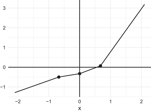
Let us limit our attention to PL functions $H(x)$ that are continuous, so that their graphs consist of a finite number of line segments that are glued together at the end points. Figure 1 depicts one such PL function, where four line segments with different slopes are joined together. Now, assume $Z$ is a standard normal variable, $Z\sim N(0,1)$. Consider the random variable $Y:=H(Z)$, which is generally non-normal. Since $Y$ is based on two analytically simple and well-known concepts, that of a standard normal variable and that of piecewise linearity, many aspects of the distribution of $X$ are amenable to analytical and computational treatment. For instance, there are exact and computationally tractable formulas for the mean, variance, skewness, and kurtosis of $Y$. The same tractability holds for the bivariate case. That is, define $Y_1:=H(Z_1)$ and $Y_2:=H(Z_2)$, where $(Z_1,Z_2)$ is a bivariate normal vector. Then, as outlined below, we may use straightforward formulas to calculate the covariance between $Y_1$ and $Y_2$. In the following, we refer to the piecewise linear simulation approach as PLSIM.

Figure 1. Graph of the continuous piecewise linear function $H_1(x)$

This article is organized as follows. We next review simulation techniques for non-normal data with pre-specified population covariance matrix. We then present our method formally, and include some illustrations in this discussion. A data illustration is thereafter given. We finally discuss strengths and limitations of PLSIM. Some R (R Core Team, 2020) code is provided in the text, and complete R code is provided in the supplemental material.

Simulating multivariate data with pre-specified covariance matrix

Given the importance of variances and covariances in factor analysis and SEM, it is not surprising that several methods have been proposed for drawing random samples from multivariate distributions whose covariance matrix is fixed. The most popular approach is the transform of Vale and Maurelli (1983), which starts with a multivariate normal vector and then applies polynomial transforms in each coordinate. The polynomials are so chosen as to produce given univariate skewness and kurtosis in the resulting vector. If feasible, the method identifies the correlation matrix in the multivariate normal vector that ensures that the polynomially transformed variables have the required covariance matrix. A thorough theoretical study of the Vale-Maurelli (VM) transform is given by Foldnes and Grønneberg (2015). The VM transform is the default method for generating non-normal data in commercial software such as EQS (Bentler, 2006) and LISREL (Jöreskog & Sörbom, 2006), and in the R package lavaan (Rosseel, 2012).

Recently, several alternative methods that also control the moments have been developed. The independent generator approach proposed by Foldnes and Olsson (2016) is available in the R package covsim (Grønneberg et al., 2021), and can match pre-specified univariate skewness and kurtosis. It offers more flexibility than VM, since many possible marginal distributions are attainable. Based on the independent generator idea, Qu et al. (2019) recently proposed a method which controls multivariate skewness and kurtosis, available in the R package mnonr (Qu & Zhang, 2020).

Both VM and the independent generator approach allows the asymptotic covariance matrix of the empirical covariances to be exactly calculated (Foldnes & Grønneberg, 2017). This means that the population-level properties of standard errors and fit statistics in SEM models may be exactly calculated using well-known formulas (Browne, 1984).

The above methods have in common with PLSIM that only some lower-order moments of the univariate distributions are controlled. Mair et al. (2012) offered a different approach, based on the concept of a copula. A copula is a multivariate distribution with uniform marginals on [0,1]. In general, multivariate distributions may be split up into a copula component and the univariate distributions. In the Mair et al. (2012) approach the marginals are specified together with the copula class, but in a final step the simulated vector is obtained by pre-multiplication with a matrix in order to reach the target covariance, leading to perturbations in the marginal distributions. We are aware of two approaches that allow complete control over the univariate distributions. First, the NORTA method of Cario and Nelson (1997), which is implemented in package SimCorMultRes (Touloumis, 2016). In common with VM and PLSIM, it is based on generating multivariate normal data and then transforming each variable according to univariate specifications. A limitation of this method is that it can only produce data with a normal copula. Second, the VITA method of Grønneberg and Foldnes (2017), implemented in package covsim (Grønneberg et al., 2021), fully specifies the marginal distributions. In addition, since VITA is based on regular vine distributions, the user may specify for each variable pair the (conditional) copula. The VITA approach is particularly suited for ordinal data simulation, as recently demonstrated by Foldnes and Grønneberg (2021).

Piecewise linear simulation: The univariate case

In this section, we consider a random variable that is stochastically represented as a PL function of a standard normal variable $Z$. A general expression for a PL function consisting of $d$ line segments is

(1) $H(x)=\sum _{i=1}^d[a_{i}x+b_i]I\{{\gamma }_{i-1}<x\le {\gamma }_i\},$(1)

where ${\gamma }_0=-\mathrm{\infty },{\gamma }_d=\mathrm{\infty }$. The indicator function $I\{A\}$ evaluates to $1$ if $A$ is true, and to $0$ otherwise. The $\gamma$ are breakpoints where function evaluation shifts from one affine function to another. The $d$ line segments have slopes denoted by $a_i$ and $y$-intercepts denoted by $b_i$. The requirement that $H(x)$ be continuous means that $b_{i+1}=(a_i-a_{i+1}){\gamma }_i+b_i$ for $i=1,\dots ,d$. Therefore, $H(x)$ is parameterized by the $a$ and $\gamma$ vectors, in addition to $b_1$ (a total of $2d$ parameters).

As an example, consider the graph in Figure 1, which depicts the following function, where $d=4$:

(2) $H_1(x)=\left\{\begin{array}{cc}0.552\cdot x-0.127& \mathrm{i}\mathrm{f}x<-0.674\\ 0.258\cdot x-0.325& \mathrm{i}\mathrm{f}-0.674\le x<0\\ 0.585\cdot x-0.325& \mathrm{i}\mathrm{f}0\le x<0.674\\ 2.185\cdot x-1.404& \mathrm{i}\mathrm{f}x>0.674\end{array}\right..$(2)

In this example the breakpoints are $-0.674,0$, and $0.674$. The breakpoints are regular in the sense that they correspond to quantiles of regularly spaced probabilities ($.25,.5$, and $.75$) for the normal distribution. Note that all the slopes in this example are positive, so that $H_1$ is a monotone function.

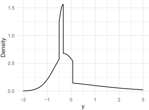
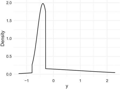
We now assume that $Z\sim N(0,1)$ is a standard normal variable, and define the random variable

(3) $Y=H(Z)=\sum _{i=1}^d[a_{i}Z+b_i]I\{{\gamma }_{i-1}<Z\le {\gamma }_i\}.$(3)

The cumulative distribution and density functions of $Y$ may be deduced following straightforward arguments (See also Foldnes & Grønneberg, 2015, Prop.1). For instance, the density may, without further assumptions, be calculated as

(4) $f(y)=\sum _{i=1}^d|a_i{|}^{-1}\varphi ((y-b_i)/a_i)I\{{\gamma }_{i-1}<(y-b_i)/a_i\le {\gamma }_i\},$(4)

where $\varphi ()$ is the density function of a standard normal variable. Figure 2 depicts the density of $H_1(Z)$. It is evident that the four line segments in $H_1(Z)$ contribute separately to the density, producing rather pronounced shifts in the density curve.

Figure 2. The density of $Y=H_1(Z)$

In order to calculate the moments of $Y$, it is useful to first obtain the conditional moments $m_k^i:=\mathrm{E}(Z^k|{\gamma }_{i-1}<Z\le {\gamma }_i)$, that is, the moments of a truncated normal variable. These may be obtained with the following recursive formula (Burkardt, 2014; Orjebin, 2014), where we initialize by $m_{-1}^i=0$ and $m_0^i=1$:

$m_k^i=(k-1)m_{k-2}^i-\frac{{\gamma }_i^{k-1}\varphi ({\gamma }_i)-{\gamma }_{i-1}^{k-1}\varphi ({\gamma }_{i-1})}{\mathrm{\Phi }({\gamma }_i)-\mathrm{\Phi }({\gamma }_{i-1})},$

where $\mathrm{\Phi }()$ is the cumulative distribution function of a standard normal variable. Now, to calculate the $k$-th moment of $Y$, we apply the following formula, which is derived in Appendix A:

(5) $\mathrm{E}(Y^k)=\sum _{i=1}^d\sum _{j=0}^k\left(\begin{array}{c}k\\ j\end{array}\right)a_i^{k-j}{b}_i^j(\mathrm{\Phi }({\gamma }_i)-\mathrm{\Phi }({\gamma }_{i-1}))m_{k-j}^i.$(5)

Using this formula, the first four centralized moments of $Y=H_1(Z)$ from Equation (2)(2) $H_1(x)=\left\{\begin{array}{cc}0.552\cdot x-0.127& \mathrm{i}\mathrm{f}x<-0.674\\ 0.258\cdot x-0.325& \mathrm{i}\mathrm{f}-0.674\le x<0\\ 0.585\cdot x-0.325& \mathrm{i}\mathrm{f}0\le x<0.674\\ 2.185\cdot x-1.404& \mathrm{i}\mathrm{f}x>0.674\end{array}\right..$(2) are

$\mathrm{E}(Y)=0,\mathrm{E}(Y^2)=1$

$\mathrm{E}(Y^3)=2,\mathrm{E}(Y^4)=8.$

In other words, $Y$ is a zero mean unit variance random variable whose skewness is $\mathrm{E}(Y^3)/\mathrm{E}(Y^2{)}^{3/2}=2$ and whose excess kurtosis is $\mathrm{E}(Y^4)/\mathrm{E}(Y^2{)}^2-3=5$.

We have shown how to calculate the moments of a given PL random variable. However, in simulation applications we need to move in the opposite direction: We first specify the moments, and then we search for a PL function that generates the pre-specified moments. That is, we use a fast numerical routine to calibrate $H_1(x)$, based on the formula in Equation (5)(5) $\mathrm{E}(Y^k)=\sum _{i=1}^d\sum _{j=0}^k\left(\begin{array}{c}k\\ j\end{array}\right)a_i^{k-j}{b}_i^j(\mathrm{\Phi }({\gamma }_i)-\mathrm{\Phi }({\gamma }_{i-1}))m_{k-j}^i.$(5) . For given breakpoints, slope values $a$ and $y$-intercepts $b$, this equation allows us to calculate the first four moments of $Y=H(Z)$. If we are given pre-specified values $\mu$, ${\sigma }^2$, ${\tilde{\mu }}_3$, and ${\tilde{\mu }}_4$ for mean, variance, skewness, and excess kurtosis, respectively, we can therefore use numerical optimization to minimize

$(\mathrm{E}(Y^3)/\mathrm{E}(Y^2{)}^{3/2}-{\tilde{\mu }}_3{)}^2+(\mathrm{E}(Y^4)/\mathrm{E}(Y^2{)}^2-{\tilde{\mu }}_3{)}^2$

as a function of $a_1,\dots ,a_d$. The above expression is not dependent upon the specific $b$-values, but we assume that these are such that $H(x)$ is continuous in each optimization step. The final step involves shifting the $b_i$ so that $\mathrm{E}(Y)=\mu$, and scaling the $a_i$ so that $\mathrm{E}(Y^2)={\sigma }^2+{\mu }^2$. The optimization routine has been implemented in the function rPLSIM in package covsim Foldnes and Grønneberg (2020b). The default setting of rPLSIM is to use three regularly spaced break-points. We here demonstrate how one may request a sample of size $1000$ from a population with skewness $2$ and excess kurtosis $5$, where the PL function is forced to be monotonous:

library(covsim)

library(psych)#for sample skew/kurtosis

set.seed(1)

res <- rPLSIM(N = 10^3, sigma.target = 1, skewness = 2, + excesskurtosis =5, monot = TRUE)

sim.sample <- res[[1]][[1]]# a simulated sample

skew(sim.sample)

kurtosi(sim.sample)

res[[2]]$\mathrm{\$}a;res[[2]]$$b#print slopes and intercepts

In the output below we see that the sample skewness and excess kurtosis values are close to the population values. Also, in the second element of the output we can inspect the fitted slope and intercept values, which agree with the values in Equation (2)(2) $H_1(x)=\left\{\begin{array}{cc}0.552\cdot x-0.127& \mathrm{i}\mathrm{f}x<-0.674\\ 0.258\cdot x-0.325& \mathrm{i}\mathrm{f}-0.674\le x<0\\ 0.585\cdot x-0.325& \mathrm{i}\mathrm{f}0\le x<0.674\\ 2.185\cdot x-1.404& \mathrm{i}\mathrm{f}x>0.674\end{array}\right..$(2) :

[1] 1.973825

[1] 4.987873

[1] 0.5519887 0.2583700 0.5849776 2.1849716

[1] −0.1271060 −0.3251488 −0.3251488 −1.4043284

Matching pre-specified mean, variance, skewness, and kurtosis

In the example above the slopes $a_1,\dots ,a_4$ and the $y$-intercepts $b_1,\dots ,b_4$ were carefully chosen so that $Y=H_1(Z)$ has mean zero, unit variance, skewness $2$ and excess kurtosis $5$. One reason for choosing the first four moments in this way was to produce a condition of non-normality where the VM transform is not helpful, since the third-order Fleishman polynomial cannot produce skewness $2$ in combination with excess kurtosis of $5$. Using the lavaan package for calibration of Fleishman polynomials yields:

library(lavaan)

res <- simulateData(“x1^~~x2,” skewness = 2, + kurtosis = 5)

lavaan WARNING: ValeMaurelli1983 method

+ did not convergence,

+ or it did not find the roots

So the skewness $2$, kurtosis $5$ case illustrates that there are conditions in which VM is infeasible but that are still within reach of PLSIM.

Given the flexibility of piecewise linear functions, it is not surprising that even with the same breakpoints, there are other PL functions that produce the same first four moments as $H_1(x)$. For instance, we may relax the monotonicity constraint:

res <- rPLSIM(N = 10^3, sigma.target = 1,

+ skewness = 2, excesskurtosis =5, monot = FALSE)

res[[2]]$a[[1]]

[1] 0.8500105 −0.9079488 1.2142742 2.1681442

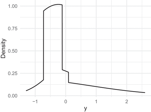
The result is a non-monotonous function $H_2(x)$ depicted in Figure 3, which ensures that $Y_2=H(Z)$ also has zero mean, unit variance, skewness 2 and excess kurtosis 5. The density of $Y_2$ is depicted in Figure 4. We observe that although $Y_1$ and $Y_2$ share the first four moments, their densities are quite dissimilar.

Figure 3. Graph of the piecewise linear function $H_2(x)$.

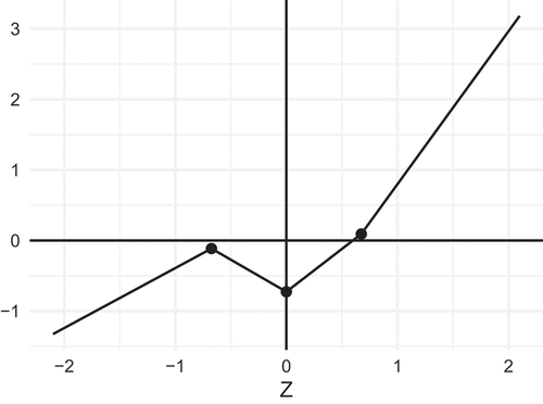
Figure 4. The density of $Y=H_2(Z)$.

To further illustrate the flexibility of piecewise linear transforms, we next specify skewness 2 and excess kurtosis 4. With the default breakpoint settings, as also used in $H_1(x)$, our routine did not identify a PL that attained these skewness and excess kurtosis values. To find a valid PL function the breakpoints therefore need to be altered, either by introducing more line segments, or by keeping d = 4 and changing the location of the breakpoints. In our case, the latter was a viable option:

g <- list(c(−2,0.5, 2))

res <- rPLSIM(N = 10^3, sigma.target = 1,

+ skewness = 2, excesskurtosis =4,

+ monot = FALSE, gammalist = g) res[[2]]$a[[1]]

[1] 1.350564 0.201702 2.284732 1.398601

For the set of feasible breakpoints ${\gamma }_1=-2,{\gamma }_2=0.5$, and ${\gamma }_3=2$, the function $H_3(x)$ depicted in Figure 5 produces the density for $Y_3=H_3(Z)$ depicted in Figure 6. This density has skewness $2$ and excess kurtosis $4$. Note that, although we did not constrain the routine to monotonous solutions, the result is still monotonous in this special case.

Figure 5. Graph of the piecewise linear function $H_3(x)$.

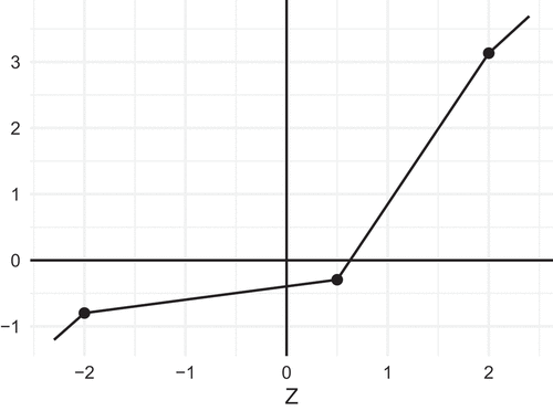
Figure 6. The density of $Y=H_3(Z)$.

The generality of univariate PLSIM

As exemplified above, PLSIM accommodates a much larger class of univariate marginal distributions than those provided under the VM transform. In fact, PLSIM may approximate to arbitrary precision the distribution $F$ of any continuous random variable $X$. For, given the quantile function $F^{-1}(u)=inf\{x:F(x)=u\}$, $0<u<1$, then $F^{-1}(U)\sim X$, provided $U$ is a uniform variable on $[0,1]$. Therefore, $F^{-1}(\mathrm{\Phi }(Z))\sim X$, where $Z\sim N(0,1)$ (Shorack & Wellner, 2009, Theorem 1, p. 3). With increasing number of breakpoints we can approximate the function $F^{-1}(\mathrm{\Phi }(x))$ using a PL function $H(x)$ arbitrarily well. It then follows that $H(Z)$ will converge in distribution to $F$ as the number of breakpoints increases, provided the breakpoints and line segments are suitably chosen.

The bivariate case

In the previous section, we demonstrated how a PL function $H(x)$ could be fitted to accommodate univariate moments for the random variable $Y=H(Z)$. In this section we move to the bivariate case where we consider $2$-dimensional random vectors

$Y=(Y,\tilde{Y}){ }^{\mathrm{\prime }}=(H(Z),\tilde{H}(\tilde{Z})){ }^{\mathrm{\prime }},$

where each coordinate is a PL transform of a standard normal variable. Moreover, $Z$ and $\tilde{Z}$ are assumed to be bivariate normally distributed and have correlation $\rho$. We assume, without loss of generality, that $H(x)$ and $\tilde{H}(x)$ are such that $Y=H(Z)$ and $\tilde{Y}=\tilde{H}(\tilde{Z})$ each has zero mean and unit variance.

Next  consider  the  covariance/correlation   between $Y=H(Z)={\sum }_{i=1}^d[a_{i}Z+b_i]I\{{\gamma }_{i-1}<Z\le {\gamma }_i\}$ and $\tilde{H}(\tilde{Z})={\sum }_{j=1}^{\tilde{d}}[{\tilde{a}}_j\tilde{Z}+{\tilde{b}}_j]I\{{\tilde{\gamma }}_{j-1}<\tilde{Z}\le {\tilde{\gamma }}_j\})$. For less notational burden, we let $R_{i,j}$ denote the rectangle $({\gamma }_{i-1},{\gamma }_i]\times ({\tilde{\gamma }}_{j-1},{\tilde{\gamma }}_j]$. Then,

$\sum _{i=1}^d[a_{i}Z+b_i]I\{{\gamma }_{i-1}<Z\le {\gamma }_i\}\sum _{j=1}^{\tilde{d}}[{\tilde{a}}_j\tilde{Z}+{\tilde{b}}_j]I\{{\tilde{\gamma }}_{j-1}<\tilde{Z}\le {\tilde{\gamma }}_j\}$

$=\sum _{i=1}^d\sum _{j=1}^{\tilde{d}}[a_{i}Z+b_i][{\tilde{a}}_j\tilde{Z}+{\tilde{b}}_j]I\{(Z,\tilde{Z})\in R_{i,j}\}$

$=\sum _{i=1}^d\sum _{j=1}^{\tilde{d}}[a_i{\tilde{a}}_{j}Z\tilde{Z}+a_i{\tilde{b}}_{j}Z+b_i{\tilde{a}}_j\tilde{Z}+b_i{\tilde{b}}_j]I\{(Z,\tilde{Z})\in R_{i,j}\}.$

This gives

(6) $\mathrm{C}\mathrm{o}\mathrm{v}(H(Z),\tilde{H}(\tilde{Z}))=\mathrm{E}(H(Z)\tilde{H}(\tilde{Z}))$(6)

$=\sum _{i=1}^d\sum _{j=1}^{\tilde{d}}[a_i{\tilde{a}}_j\mathrm{E}(Z\tilde{Z}I\{(Z,\tilde{Z})\in R_{i,j}\})+$

$a_i{\tilde{b}}_j\mathrm{E}(ZI\{(Z,\tilde{Z})\in R_{i,j}\})+$

$b_i{\tilde{a}}_j\mathrm{E}(\tilde{Z}I\{(Z,\tilde{Z})\in R_{i,j}\})+$

$b_i{\tilde{b}}_j\mathrm{E}(I\{(Z,\tilde{Z})\in R_{i,j}\})]$

$=\sum _{i=1}^d\sum _{j=1}^{\tilde{d}}[a_i{\tilde{a}}_j\mathrm{E}(Z\tilde{Z}|(Z,\tilde{Z})\in R_{i,j})+$

$a_i{\tilde{b}}_j\mathrm{E}(Z|(Z,\tilde{Z})\in R_{i,j})+$

$b_i{\tilde{a}}_j\mathrm{E}(\tilde{Z}|(Z,\tilde{Z})\in R_{i,j})+$

$b_i{\tilde{b}}_j]\cdot P((Z,\tilde{Z})\in R_{i,j}).$

Procedures for calculating the moments

$\mathrm{E}(Z\tilde{Z}|(Z,\tilde{Z})\in R)\mathrm{a}\mathrm{n}\mathrm{d}\mathrm{E}(Z|(Z,\tilde{Z})\in R)$

of a truncated bivariate normal variable is a well-studied problem (e.g., Leppard & Tallis, 1989). In our implementation we use the R package tmvtnorm (Wilhelm & Manjunath, 2015) to calculate these moments.

It is important to notice that the expression in Equation (6)(6) $\mathrm{C}\mathrm{o}\mathrm{v}(H(Z),\tilde{H}(\tilde{Z}))=\mathrm{E}(H(Z)\tilde{H}(\tilde{Z}))$(6) , in addition to being dependent upon the slopes, $y$-intercepts and breakpoints in $H(x)$ and $\tilde{H}(x)$, also depends on an additional parameter, namely $\rho$, the intermediate correlation between $Z$ and $\tilde{Z}$. We emphasize this in notation by writing $\mathrm{C}\mathrm{o}\mathrm{v}(H(Z),\tilde{H}(\tilde{Z});\rho )$.

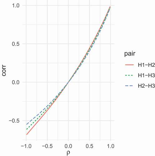
We next illustrate the dependency of $\mathrm{C}\mathrm{o}\mathrm{v}(H(Z),\tilde{H}(\tilde{Z});\rho )$ on $\rho$. We consider the three PL functions $H_1(x),H_2(x)$, and $H_3(x)$ introduced in the previous section. For values of $\rho$ between $-1$ and $1$, we calculated the correlation $\mathrm{C}\mathrm{o}\mathrm{v}(H_1(Z),H_2(\tilde{Z});\rho )$, $\mathrm{C}\mathrm{o}\mathrm{v}(H_1(Z),H_3(\tilde{Z});\rho )$, and $\mathrm{C}\mathrm{o}\mathrm{v}(H_2(Z),H_3(\tilde{Z});\rho )$. In Figure 7 we graphically depict the dependence of the correlations upon the correlation $\rho$ between $Z$ and $\tilde{Z}$. Clearly, combining $H_1(x)$ and $H_2(x)$ yields the largest possible range of correlations, although there is no way to produce a correlation below$-.68$ for this pair of PL transforms. Combining $H_2(x)$ and $H_3(x)$ yields the smallest range, with the lowest attainable correlation being $-.55$. The figure demonstrates that not all correlations are attainable once the univariate specification of skewness and excess kurtosis have been given.

Figure 7. The correlation among piecewise linear transforms of bivariate normal variables with correlation $\rho$.

The PLSIM simulation procedure

In the previous sections, we demonstrated how a PL function could be fitted to accommodate univariate moments of the simulated variable $Y=H(Z)$, and how to calculate the covariance among two such variables. We now move to the full multivariate case and consider $p$-dimensional random vectors

(7) $Y=(H_1(Z_1),H_2(Z_2),\dots ,H_p(Z_p)){ }^{\mathrm{\prime }},$(7)

where each coordinate $H_i(Z_i)$ is a PL transform of a standard normal variable,¹ $Z_i\sim N(0,1)$. We assume, without loss of generality, that the $H_i(x)$ functions ($i=1,\dots ,p$) have been calibrated so that $H_i(Z_i)$ has zero mean and unit variance. We also assume that $Z=(Z_1,\dots ,Z_p)$ is multivariate normally distributed with standardized marginals and a covariance matrix equal to ${\mathrm{\Sigma }}_Z$. Note that ${\mathrm{\Sigma }}_Z$ is in fact a correlation matrix containing $p(p-1)/2$ non-redundant off-diagonal elements.

The steps in PLSIM are as follows:

1. The user specifies

• (a) Univariate properties (e.g., skewness and excess kurtosis) of each marginal variable $Y_1,\dots ,Y_p$.

• (b) A target correlation matrix $\mathrm{\Sigma }$.

1. (2) The PL functions $H_1,\dots ,H_p$ are calibrated to match the properties specified in step 1(a).

2. (3) For each correlation ${\rho }_{i,j}$, $1\le i<j\le p$ in $\mathrm{\Sigma }$, we numerically determine a correlation ${\rho }_{i,j}^Z$ among $Z_i$ and $Z_j$ so that $H_i(Z_i)$ and $H_j(Z_j)$ have correlation ${\rho }_{i,j}$.

3. (4) The matrix ${\mathrm{\Sigma }}_Z$ is formed from entries ${\rho }_{i,j}^Z$. A random sample from the multivariate normal distribution with zero mean and covariance matrix ${\mathrm{\Sigma }}_Z$ is drawn. We apply the functions $H_i(x)$, $i=1,\dots ,p$, coordinate-wise to the random sample to obtain our PLSIM sample.

There are two ways the above procedure may fail to complete. First, in Step 2, we may fail to identify a $H_i(x)$ for some $i=1,\dots ,p$, that reaches the given skewness and kurtosis values. Although we may then change the breakpoint locations or increase the number of breakpoints, it is computationally burdensome to run PLSIM with, say, 20 breakpoints in each of 40 variables. In the R implementation provided in the supplemental material, the default number of breakpoints is $3$, which are regularly placed ($-0.674,0,0.674$) so that each line segment is associated with the same probability $.25$. In our experiments, this seems to offer a reasonable compromise between computational tractability and flexibility across various skewness, kurtosis and correlations combinations.

The second way the above PLSIM procedure may fail, is in Step 4, should ${\mathrm{\Sigma }}_Z$ be negative definite. That is, it may happen that ${\mathrm{\Sigma }}_Z$ is not a proper correlation matrix. The reason for this is that we, for computational simplicity, calibrate the entries in ${\mathrm{\Sigma }}_Z$ independently. The alternative is full simultaneous calibration of all the entries, under the additional restraint of positive definiteness. However, we did not find this option viable in our numerical experiments. The issue of the intermediate matrix not being a proper correlation matrix arises also in the VM procedure. We here propose a simple solution to this problem, which is applicable to both PLSIM and VM. If ${\mathrm{\Sigma }}_Z$ is negative definite, we calculate its nearest correlation matrix ${\mathrm{T}}_Z$. There are various approaches to defining ${\mathrm{T}}_Z$, and in our current implementation we use the method proposed by Higham (2002), as implemented in package Matrix (Bates & Maechler, 2019). Then, in Step 4, we replace ${\mathrm{\Sigma }}_Z$ by ${\mathrm{T}}_Z$. This means that the target covariance $\mathrm{\Sigma }$ is no longer reached. However, we may correct this by pre-multiplying the PLSIM vector $Y$ by

$P={\mathrm{\Sigma }}^{1/2}{M}^{-1/2},$

where $M$ is the implied covariance matrix of $Y=(H_1(Z_1),\dots ,H_p(Z_p)){ }^{\mathrm{\prime }}$, when the $Z_i$, $(i=1,\dots ,p)$ have covariance ${\mathrm{T}}_Z$. The square root matrices are symmetric and such that $M^{1/2}{M}^{1/2}=M$ and ${\mathrm{\Sigma }}^{1/2}{\mathrm{\Sigma }}^{1/2}=\mathrm{\Sigma }$. Note that, due to Equation (6)(6) $\mathrm{C}\mathrm{o}\mathrm{v}(H(Z),\tilde{H}(\tilde{Z}))=\mathrm{E}(H(Z)\tilde{H}(\tilde{Z}))$(6) , exact calculation of $M$ is straightforward. In most cases $P$ will be fairly close to the identity matrix, so that the marginal distributions will be only slightly modified by pre-multiplication. So the pre-specified marginal properties, e.g., skewness and kurtosis, will still be closely matched, while the covariance matrix will be exactly matched. To summarize, to avoid the problem of negative definiteness, we rewrite Step 4 above as follows:

4. The matrix ${\mathrm{\Sigma }}_Z$ is formed, with elements ${\rho }_{i,j}^Z$. If ${\mathrm{\Sigma }}_Z$ is negative definite, let ${\mathrm{T}}_Z$ denotes its closest positive definite matrix. Draw a random sample from the multivariate normal distribution with zero mean and covariance matrix ${\mathrm{\Sigma }}_Z$ (or ${\mathrm{T}}_Z$ when needed). Apply the functions $H_i(x)$, $i=1,\dots ,p$, coordinate-wise to the random sample. If ${\mathrm{T}}_Z$ was used, the final random sample is obtained by post-multiplying the random data matrix by ${\mathrm{\Sigma }}^{1/2}{M}^{-1/2}$.

On the asymptotic covariance matrix for PLSIM

As argued by Foldnes and Grønneberg (2017), it is desirable in a simulation study to specify non-normality more precisely than just reporting univariate skewness and kurtosis. Ideally, the full asymptotic covariance matrix $\mathrm{\Gamma }$ of the empirical second-order moments should be computed in each simulation condition. For SEM, access to $\mathrm{\Gamma }$ means that the population-level properties of standard errors and fit statistics may be exactly calculated using well-known formulas (Browne, 1984). For PLSIM, we here show that there are closed form formulas available from $\mathrm{\Gamma }$. Unfortunately, no presently available implementation of these formulas are able to calculate these quantities within either an acceptable running time, or at an acceptable numerical precision. New implementations will be needed for calculating $\mathrm{\Gamma }$ for PLSIM. In light of this future availability, we here sketch how $\mathrm{\Gamma }$ can be obtained.

Consider a random $p$-dimensional vector $Y$ whose expectation is zero and whose fourth-order moments exist. Let $\mathrm{\Sigma }$ be the covariance matrix of $Y$. Then $\mathrm{\Gamma }$ is defined as the $p(p+1)/2\times p(p+1)/2$ matrix with elements

${\mathrm{\Gamma }}_{ij,kl}=\mathrm{E}(Y_i{Y}_j{Y}_k{Y}_l)-{\mathrm{\Sigma }}_{ij}{\mathrm{\Sigma }}_{kl},$

where all or some indices are allowed to be equal. To obtain $\mathrm{\Gamma }$ under PLSIM, we need to perform calculations for the expectation similar to the deductions in Equation (6)(6) $\mathrm{C}\mathrm{o}\mathrm{v}(H(Z),\tilde{H}(\tilde{Z}))=\mathrm{E}(H(Z)\tilde{H}(\tilde{Z}))$(6) . The full expression for $\mathrm{E}(H_i(Z_i)H_j(Z_j)H_k(Z_k)H_l(Z_l))$ is a linear combination of elements of the type

$\mathrm{E}(Z_i{Z}_j{Z}_k{Z}_l\cdot I\{(Z_i,Z_j,Z_k,Z_l)\in R\})$

(8) $=\mathrm{E}(Z_i{Z}_j{Z}_k{Z}_l|(Z_i,Z_j,Z_k,Z_l)\in R)P((Z_i,Z_j,Z_k,Z_l)\in R),$(8)

where $R$ is a four-dimensional rectangle defined by four pairs of breakpoints in $H_i(x),H_j(x),H_k(x),$ and $H_l(x)$, and again indices are allowed to be equal. We therefore need to calculate higher-order moments of a truncated multivariate normal vector, and there exist both exact recursive and non-recursive formulas for this task. A numerical routine implementing the recursive formulas is found in package MomTrunc (Galarza et al., 2021), and succeeds in calculating a subset of the required moments at an acceptable speed and precision. However, in our experiments, tri- and four-variate moments as calculated by MomTrunc are sometimes not satisfactory, a finding echoed by Ogasawara (2021), who developed non-recursive formulas which can be used to calculate higher-order moments of a truncated normal vector to arbitrary precision. Unfortunately, the only available implementation for the formulas in Ogasawara (2021), which is given in the supplementary material of Ogasawara (2021), takes an excessive long time to terminate in one of the cases we need, namely when all indices in Equation (8)(8) $=\mathrm{E}(Z_i{Z}_j{Z}_k{Z}_l|(Z_i,Z_j,Z_k,Z_l)\in R)P((Z_i,Z_j,Z_k,Z_l)\in R),$(8) are distinct, and genuine four-dimensional integration is required. There is therefore no available implementation of an algorithm capable of computing $\mathrm{\Gamma }$ in reasonable time, and we therefore do not provide a function to calculate $\mathrm{\Gamma }$ in our implementation. This will be added when future efficiency improvements in the procedure proposed by Ogasawara (2021) is made available. A rough approximation to $\mathrm{\Gamma }$ can be obtained, as always, by direct simulation from PLSIM.

Limitations

As argued above, the univariate generality of PLSIM is only limited by computational considerations. However, this is not the case in terms of multivariate dependency properties, as PLSIM takes a multivariate normal random vector and apply only coordinate-wise transformations. Since the transformation from $Z$ to $Y$ has no interaction between the coordinates, this restricts the multivariate dependency properties of $Y$, as shown in Foldnes and Grønneberg (2015).

Recall that the copula of a continuous random vector $(X_1,\dots ,X_p){ }^{\mathrm{\prime }}$ is the distribution of $(F_1(X_1),\dots ,F_d(X_p)){ }^{\mathrm{\prime }}$ where $F_1,\dots ,F_p$ are the marginal cumulative distribution functions of $X_1,\dots ,X_p$. In the case where each of the coordinate-wise transformations $H_1,\dots ,H_p$ are monotonous, the copula of the PLSIM random vector $Y$ of Equation (7)(7) $Y=(H_1(Z_1),H_2(Z_2),\dots ,H_p(Z_p)){ }^{\mathrm{\prime }},$(7) is exactly normal, meaning that it has the same copula as the multivariate normal vector $Z$.

A recent discovery (Grønneberg & Foldnes, 2019) warns against the widespread practice of using VM in robustness studies for ordinal SEM. In many relevant cases encountered in the simulation literature, VM has the normal copula, which in ordinal SEM has the unfortunate consequence of making the ordinal vector generated by discretizing a VM random vector numerically equal to a discretization of an exactly normal random vector. The distribution of the manifest variables in ordinal SEM is a function only of the copula of the latent continuous vector at certain points (Foldnes & Grønneberg, 2019, 2020a, 2021; Grønneberg & Foldnes, 2021; Grønneberg & Moss, 2021). Since PLSIM will have a normal copula when each $H_1,\dots ,H_p$ are monotonous, the discovery of Grønneberg and Foldnes (2019) also applies to PLSIM. Therefore, PLSIM for simulation studies with ordinal SEM is not recommended, and if used, must be used for non-monotonous $H_1,\dots ,H_p$. One important exception is if a normal copula is desired. For instance, Grønneberg and Foldnes (2021) employed a simple bivariate PLSIM distribution to illustrate that ordinal SEM estimation is biased unless knowledge of all latent marginal distributions is provided. In that case, profiting from PLSIM’s marginal flexibility, a bivariate vector $Y$ was constructed who followed a two-factor model, while the bivariate generator vector $Z$ followed a one-factor model. Since $Y$ had a normal copula, all normal theory methods based on discretizing $Y$ estimate features of $Z$ and not $Y$, illustrating the impossibility of identifying even the number of factors in ordinal SEM without latent marginal knowledge.

In general, PLSIM distributions are contained in the class investigated by Foldnes and Grønneberg (2015), as $Y$ is the coordinate-wise transformation of a continuous random vector $Z$, where each transformation is piecewise strictly monotonous over a finite set of intervals. In PLSIM, we have that $Z$ is multivariate normal with standardized marginals, and the transformations are straight lines in each interval segment. When some of the coordinate-wise transformations are non-monotonous, the copula of $Y$ is not exactly normal, but the multivariate distribution is still strongly connected to the normal generator variable $Z$, and for example, $Y$ cannot have what is known as tail dependence, see Section 3.3 of Foldnes and Grønneberg (2015).

The main limitation of PLSIM is therefore its close connection to the normal distribution in terms of copula properties. This limitation may be remedied by replacing the normal random vector with another class of distributions capable of detailed control of lower moments, and with computationally feasible formulas for conditional distributions over rectangles. As mentioned above, calculating the fourth-order moments contained in $\mathrm{\Gamma }$ leads to serious computational challenges even when $Z$ is multivariate normal. It therefore seems that such extensions would either be restricted to very simple distributional classes which would limit its usefulness, or would depend on as of yet unavailable numerical methods.

A comparison of Fleishman polynomials and PLSIM

As discussed above, PLSIM and VM are similar in terms of multivariate dependency, as both are generated by coordinate-wise transformations of a normal random vector. We here further inquire into the univariate distributional differences between PLSIM and VM. In the latter procedure, the marginal distributions are generated by third-order polynomial transformations as proposed by Fleishman (1978). Third-order polynomials $f(x)$ grow more quickly to $\pm \mathrm{\infty }$ as $x\to \pm \mathrm{\infty }$ than PL functions, who involve only a simple scale-and-shift of the identity function. In this sense PL functions are more stable transformations compared to Fleishman polynomials, yet they preserve the capability of approximating general functions to arbitrary precision. The stability concerns the tails of the resulting univariate distributions. As implied from Equation (4)(4) $f(y)=\sum _{i=1}^d|a_i{|}^{-1}\varphi ((y-b_i)/a_i)I\{{\gamma }_{i-1}<(y-b_i)/a_i\le {\gamma }_i\},$(4) , PL functions have the same tail behavior as a normal distribution. That is, when $y\to \mathrm{\infty }$, PL density approaches zero as $a_d\varphi ((y-b_d)/a_d)$, and when $y\to -\mathrm{\infty }$, the density goes to zero as $a_1\varphi ((y-b_1)/a_1)$. That is, in PL functions, the tail behavior is still driven solely by the quick decrease to zero of $\varphi (y)=(2\pi {)}^{-1/2}exp(-y^2/2)$. This is not the case for VM, which has heavier tails due to the third-order transformation. Whether heavier tails are desirable, and whether considerations as $|y|\to \mathrm{\infty }$ are relevant or not, depends on the application.

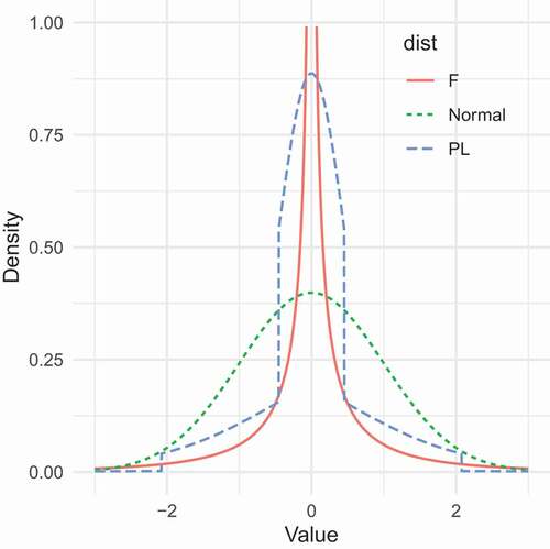
Let us consider in a concrete example the relation between a normal ($Z$), a PL ($Y_{PL}$) and a Fleishman ($Y_F$) variable. The simplest case of a Fleishman polynomial is the standardized third-order transformation $(Z^3-{\mu }_3)/{\sigma }_3$. We have ${\mu }_3=\mathrm{E}{Z}^3=0$ and ${\sigma }_3=\sqrt{\mathrm{V}\mathrm{a}\mathrm{r}{Z}^3}=\sqrt{\mathrm{E}{Z}^6-{(\mathrm{E}{Z}^3)}^2}=\sqrt{\mathrm{E}{Z}^6}=\sqrt{15}$. Therefore, $Y_F=Z^3/\sqrt{15}$. The excess kurtosis of $Y_F$ is extreme, namely $\mathrm{E}{Y}_F^4-3=({15}^{-1/2}{)}^4\mathrm{E}{Z}^{3\cdot 4}-3=(15{)}^{-2}\mathrm{E}{Z}^{12}-3=46.2-3=$ 43.2. The density of $Y_F$ is $y\mapsto \varphi ((15{)}^{1/6}{y}^{1/3})(15{)}^{1/6}(1/3)y^{-2/3}$. While the term $y^{-2/3}$ quickens the convergence to zero, the $y^{1/3}$ term inside $\varphi$ slows down convergence, and this is the dominant term. We also fitted, using breakpoints $-3,-2,-1,1,2,$ and $3$, a PL function $H(x)$ so that $Y_{PL}=H(Z)$ had zero mean, unit variance, skew zero, and excess kurtosis 43.2. Figure 8 depicts the density curves of the three densities. Clearly, although the Fleishman and the PL distribution have common moments up to the fourth order, their distributions differ markedly. Both distributions are more peaked and more heavy-tailed than the standard normal distribution. But the peakedness of the Fleishman polynomial is much more pronounced than that of the PL distribution. Moreover, although not depicted in the figure, for extreme values, the tails of the Fleishman polynomial are fatter than those of the PL distribution. To illustrate this point, we simulated $n={10}^7$ sample from both distributions, and found that the 99th-percentiles for the PL and Fleishman data were $2.75$ and $3.8$, respectively (see the supplemental material).

Figure 8. Graph of the density of $Z$ and the standardized version of $Z^3$ when $Z\sim N(0,1)$.

Illustration

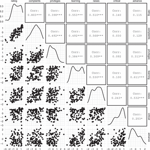
Let us illustrate PLSIM with a real-world example. The datasets package contains the dataset attitude, based on a survey given to employees in a large financial organization related to satisfaction with their supervisors. For 30 randomly chosen departments the proportion of favorable responses for each item was collected in the attitude dataset. The correlation matrix and the marginal sample skewnesses and excess kurtosi are given Table 1. Our aim here is to construct a 7-variate distribution whose correlation matrix and marginal skewness and excess kurtosis values match exactly the values in Table 1.

library(datasets)

attach(attitude)

s <- skew(attitude)

k <- kurtosi(attitude)

sigma <- cor(attitude)

set.seed(1)

res <- rPLSIM(100, sigma.target = sigma, + skewness = s, excesskurtosis = k)

sim.sample <- res[[1]][[1]]

Table 1. Correlation matrix and marginal skewnesses and excess kurtosi for the attitude dataset

	Rating	Complaints	Privileges	Learning	Raises	Critical	Advance
Rating	$1$	$.825$	$.426$	$.624$	$.590$	$.156$	$.155$
complaints		$1$	$.558$	$.597$	$.669$	$.188$	$.225$
privileges			$1$	$.493$	$.445$	$.147$	$.343$
learning				$1$	$.640$	$.116$	$.532$
raises					$1$	$.377$	$.574$
critical						$1$	$.283$
advance							$1$
skewness	−0.358	−0.215	0.379	−0.054	0.198	−0.866	0.850
kurtosis	−0.766	−0.677	−0.411	−1.223	−0.599	0.166	0.466

Note that the VM approach as implemented in lavaan is not up to this task, since it can not match the skewness and excess kurtosis of variable learning. However, with three regularly spaced thresholds, monotonous PL functions may be identified (Step 2) for each of the seven variables that match skewness and excess kurtosis exactly. In Step 3 we fit each pair of variables separately, and in Step 4 the correlations are aggregated into:

${\mathrm{\Sigma }}_Z=\left(\begin{array}{ccccccc}1& .834& .440& .643& .605& .165& .163\\ \hspace{0.17em}& 1& .570& .611& .678& .196& .233\\ \hspace{0.17em}& \hspace{0.17em}& 1& .509& .451& .156& .353\\ \hspace{0.17em}& \hspace{0.17em}& \hspace{0.17em}& 1& .656& .123& .559\\ \hspace{0.17em}& \hspace{0.17em}& \hspace{0.17em}& \hspace{0.17em}& 1& .397& .588\\ \hspace{0.17em}& \hspace{0.17em}& \hspace{0.17em}& \hspace{0.17em}& \hspace{0.17em}& 1& .309\\ \hspace{0.17em}& \hspace{0.17em}& \hspace{0.17em}& \hspace{0.17em}& \hspace{0.17em}& \hspace{0.17em}& 1\end{array}\right)$

This matrix is positive definite, so we need not pre-multiply by $P$. A sample of size $n=100$ was simulated using PLSIM, with resulting scatter plots and univariate densities depicted in Figure 9.

Figure 9. Plots for $n=100$ dataset simulated from PLSIM.

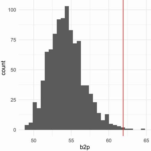
Finally, let us inspect sample estimates of kurtosis with respect to the pre-specified kurtosis values. In a generated sample, sample kurtosis will differ substantially from the specified kurtosis value. The latter holds at the population level but not in samples. To illustrate, we generated 1000 samples, each of size 30, from PLSIM. In each sample univariate kurtosis was estimated for each of the seven variables. The results are depicted in Figure 10, where each panel is associated with one variable. It is seen that sample excess kurtosis varies substantially across samples. In each panel, the vertical red line indicates population excess kurtosis. Small-sample bias of the kurtosis estimator is manifested for most variables, with general downward bias in our case. Let us also consider the $b_{2,p}$ statistic (Mardia, 1970) for multivariate kurtosis. Qu et al. (2019) proposed a simulation method where samples are generated from a distribution with pre-specified multivariate kurtosis. In our development of PLSIM, we control the univariate kurtosi, but we have no control over multivariate kurtosis. Over the same 1000 samples described above, we calculated $b_{2,p}$, with results given in Figure 11. The red line represents this statistic calculated in the attitude dataset. It is seen that the PLSIM datasets have lower $b_{2,p}$ values than the original attitude data. This illustrates that we do not control multivariate kurtosis with our method.

Figure 10. Histograms of sample estimates of univariate kurtosis based on 1000 simulated datasets of size $n=30$. The red line represents the population kurtosis derived from the attitude dataset.

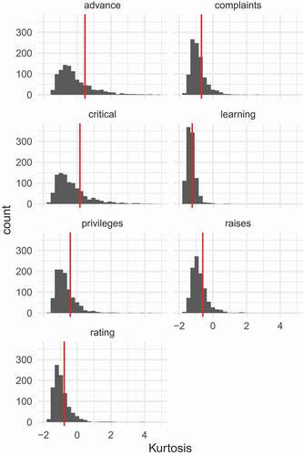
Figure 11. Histogram of multivariate kurtosis $b_{2,p}$ based on 1000 simulated datasets of size $n=30$. The red line represents $b_{2,p}$ calculated for the attitude dataset.

Conclusion

We have presented a new method to simulate univariate and multivariate non-normal data. We employ piecewise linear transforms of standard normal variables. This method is flexible since we may manipulate the slopes of the line segments in order to reach pre-specified skewness and kurtosis values. This is possible since the fourth-order moments of the transformed variable is exactly computable. The same holds for pairs of piecewise linearly transformed variables, i.e., the covariance may be calculated using exact formulas. This means that we may pairwise calibrate the correlation among the two standard normal variables in order to reach a given covariance among the transformed variables.

PLSIM has been implemented in R and is available in package covsim. We have demonstrated that PLSIM may be used in cases (e.g., skewness $2$ and excess kurtosis $4$) where the Vale-Maurelli procedure fails. PLSIM supports a flexible class of univariate distributions, since its framework is based on choosing arbitrary number and placement of breakpoints, and arbitrary line segments between the breakpoints. In our implementation the default number of line segments is four, separated by regularly spaced breakpoints. We have deduced the formulas necessary to exactly compute the asymptotic covariance matrix of the generated second-order moments under PLSIM. However, at the present time the needed routines to calculate moments of the truncated multivariate normal distributions are too slow for practical use. However, we project that this situation will be soon remedied, given the present active development around truncated multivariate moments in the field of multivariate statistics. We also proposed a simple correction to the case of negative definiteness of the intermediate correlation matrix, based on finding the nearest positive definite matrix. This correctional step may likewise be useful for extending the generality of the Vale-Maurelli procedure.

Notes

¹ $H_1,H_2,\dots ,H_p$ denote general functions of the form of Equation (1)(1) $H(x)=\sum _{i=1}^d[a_{i}x+b_i]I\{{\gamma }_{i-1}<x\le {\gamma }_i\},$(1) , and not the specific illustrative functions defined in the previous sections.

Appendix

Calculating the moments of $Y=H(Z)$Consider the random variable $Y=H(Z)$. Then

$Y^k={\left(\sum _{i=1}^d[a_{i}Z+b_i]I\{{\gamma }_{i-1}<Z\le {\gamma }_i\}\right)}^k$

$=\sum _{i=1}^d[a_{i}Z+b_i{]}^{k}I\{{\gamma }_{i-1}<Z\le {\gamma }_i\}$

$=\sum _{i=1}^d\sum _{j=0}^k\left(\begin{array}{c}k\\ j\end{array}\right)a_i^{k-j}{b}_i^j{Z}^{k-j}I\{{\gamma }_{i-1}<Z\le {\gamma }_i\}.$

Now, since

$\mathrm{E}(Z^{k}I\{{\gamma }_{i-1}<Z\le {\gamma }_i\})=$

$\mathrm{E}(Z^{k}I\{{\gamma }_{i-1}<Z\le {\gamma }_i\}|Z\le {\gamma }_{i-1})\mathrm{\Phi }({\gamma }_{i-1})+$

$\mathrm{E}(Z^{k}I\{{\gamma }_{i-1}<Z\le {\gamma }_i\}|{\gamma }_{i-1}<Z\le {\gamma }_i)(\mathrm{\Phi }({\gamma }_i)-\mathrm{\Phi }({\gamma }_{i-1}))+$

$\mathrm{E}(Z^{k}I\{{\gamma }_{i-1}<Z\le {\gamma }_i\}|{\gamma }_i<Z)(1-\mathrm{\Phi }({\gamma }_i))=$

$\mathrm{E}(Z^k|{\gamma }_{i-1}<Z\le {\gamma }_i)(\mathrm{\Phi }({\gamma }_i)-\mathrm{\Phi }({\gamma }_{i-1}))$

the $k$-th moment is

$\mathrm{E}(Y^k)=\sum _{i=1}^d\sum _{j=0}^k\left(\begin{array}{c}k\\ j\end{array}\right)a_i^{k-j}{b}_i^j\mathrm{E}(Z^{k-j}I\{{\gamma }_{i-1}<Z\le {\gamma }_i\})$

$=\sum _{i=1}^d\sum _{j=0}^k\left(\begin{array}{c}k\\ j\end{array}\right)a_i^{k-j}{b}_i^j\mathrm{E}(Z^{k-j}|{\gamma }_{i-1}<Z\le {\gamma }_i)(\mathrm{\Phi }({\gamma }_i)-\mathrm{\Phi }({\gamma }_{i-1})).$

To evaluate this expression we need to calculate the conditional moments $m_k:=\mathrm{E}(Z^k|{\gamma }_{i-1}<Z\le {\gamma }_i)$, that is, the $k$-th moment of a truncated normal variable. Mean and variance formulas are provided in Johnson et al. (1994). Higher-order moments may be obtained with the following recursive formula (Burkardt, 2014; Orjebin, 2014), where we initialize by $m_{-1}=0$ and $m_0=1$:

$m_k=(k-1)m_{k-2}-\frac{{\gamma }_i^{k-1}\varphi ({\gamma }_i)-{\gamma }_{i-1}^{k-1}\varphi ({\gamma }_{i-1})}{\mathrm{\Phi }({\gamma }_i)-\mathrm{\Phi }({\gamma }_{i-1})}.$

To sum up, we may calculate $\mathrm{E}(Y^k)$ by first using the above recursive formula to calculate the conditional moments $m_1,\dots ,m_k$. Then we apply the formula

$\mathrm{E}(Y^k)=\sum _{i=1}^d\sum _{j=0}^k\left(\begin{array}{c}k\\ j\end{array}\right)a_i^{k-j}{b}_i^j(\mathrm{\Phi }({\gamma }_i)-\mathrm{\Phi }({\gamma }_{i-1}))m_{k-j}.$

References

- Bates, D., & Maechler, M. (2019). Matrix: Sparse and dense matrix classes and methods [Computer software manual]. https://CRAN.R-project.org/package=Matrix(Rpackageversion1.2–18)
- Bentler, P. (2006). Eqs 6 structural equations program manual. Multivariate Software, Inc.
- Browne, M. W. (1984). Asymptotically distribution-free methods for the analysis of covariance structures. British Journal of Mathematical and Statistical Psychology, 37, 62–83. https://doi.org/https://doi.org/10.1111/j.2044-8317.1984.tb00789.x
- Burkardt, J. (2014). The truncated normal distribution (Tech. Rep.). Department of Scientific Computing Website, Florida State University.
- Cain, M. K., Zhang, Z., & Yuan, K.-H. (2017). Univariate and multivariate skewness and kurtosis for measuring nonnormality: Prevalence, influence and estimation. Behavior Research Methods, 49, 1716–1735. https://doi.org/https://doi.org/10.3758/s13428-016-0814-1
- Cario, M. C., & Nelson, B. L. (1997). Modeling and generating random vectors with arbitrary marginal distributions and correlation matrix (Tech. Rep.). Department of Industrial Engineering and Management Sciences, Northwestern University.
- Fleishman, A. (1978). A method for simulating non-normal distributions. Psychometrika, 43(4), 521–532. https://doi.org/https://doi.org/10.1007/BF02293811
- Foldnes, N., & Grønneberg, S. (2015). How general is the Vale–Maurelli simulation approach? Psychometrika, 80, 1066–1083. https://doi.org/https://doi.org/10.1007/s11336-014-9414-0
- Foldnes, N., & Grønneberg, S. (2017). The asymptotic covariance matrix and its use in simulation studies. Structural Equation Modeling: A Multidisciplinary Journal, 24, 881–896. doi:https://doi.org/10.1080/10705511.2017.1341320.
- Foldnes, N., & Grønneberg, S. (2019). On identification and non-normal simulation in ordinal covariance and item response models. Psychometrika, 84, 1000–1017. https://doi.org/https://doi.org/10.1007/s11336-019-09688-z
- Foldnes, N., & Grønneberg, S. (2020a). Pernicious polychorics: The impact and detection of underlying non- normality. Structural Equation Modeling: A Multidisciplinary Journal, 27, 525–543. doi:https://doi.org/10.1080/10705511.2019.1673168.
- Foldnes, N., & Grønneberg, S. (2020b). covsim: Simulate from distributions with given covariance matrix and marginal information [Computer software manual]. https://CRAN.R-project.org/package=covsim(Rpackageversion0.2.0)
- Foldnes, N., & Grønneberg, S. (2021). The sensitivity of structural equation modeling with ordinal data to underlying non-normality and observed distributional forms. Psychological Methods. (Online first). https://doi.org/https://doi.org/10.1037/met0000385
- Foldnes, N., & Olsson, U. H. (2016). A simple simulation technique for nonnormal data with prespecified skewness, kurtosis, and covariance matrix. Multivariate Behavioral Research, 51, 207–219. https://doi.org/https://doi.org/10.1080/00273171.2015.1133274
- Galarza, C. E., Kan, R., & Lachos, V. H. (2021). Momtrunc: Moments of folded and doubly truncated multivariate distributions [Computer software manual]. https://CRAN.R-project.org/package= MomTrunc (R package version 5.97)
- Grønneberg, S., & Foldnes, N. (2017). Covariance model simulation using regular vines. Psychometrika, 82, 1035–1051. https://doi.org/https://doi.org/10.1007/s11336-017-9569-6
- Grønneberg, S., & Foldnes, N. (2019). A problem with discretizing Vale-Maurelli in simulation studies. Psychometrika, 84, 554–561. https://doi.org/https://doi.org/10.1007/s11336-019-09663-8
- Grønneberg, S., & Foldnes, N. (2021). Factor analyzing ordinal items requires substantive knowledge of response marginals. Psychological Methods. (Submitted). https://doi.org/https://doi.org/10.1037/met0000385
- Grønneberg, S., Foldnes, N., & Marcoulides, K. M. (2021). covsim: An r package for simulating non-normal data for structural equation models using copulas. Journal of Statistical Software. forthcoming.
- Grønneberg, S., & Moss, J. (2021). Partial identification of latent correlations with polytomous data. Psychometrika. (Submitted).
- Higham, N. J. (2002). Computing the nearest correlation matrix—a problem from finance. IMA Journal of Numerical Analysis, 22, 329–343. https://doi.org/https://doi.org/10.1093/imanum/22.3.329
- Johnson, N. L., Kotz, S., & Balakrishnan, N. (1994). Continuous univariate distributions (Vol. 1). John Wiley & Sons.
- Jöreskog, K., & Sörbom, D. (2006). Lisrel version 8.8. lincolnwood, il: Scientific software international. Inc.
- Leppard, P., & Tallis, G. (1989). Algorithm as 249: Evaluation of the mean and covariance of the truncated multinormal distribution. Journal of the Royal Statistical Society. Series C, Applied Statistics, 38, 543–553.
- Mair, P., Satorra, A., & Bentler, P. M. (2012). Generating Nonnormal Multivariate Data Using Copulas: Applications to SEM. Multivariate Behavioral Research, 47, 547–565. https://doi.org/https://doi.org/10.1080/00273171.2012.692629
- Mardia, K. (1970). Measures of multivariate skewness and kurtosis with applications. Biometrika, 57, 519–530. https://doi.org/https://doi.org/10.1093/biomet/57.3.519
- Micceri, T. (1989). The unicorn, the normal curve, and other improbable creatures. Psychological Bulletin, 105, 156.
- Ogasawara, H. (2021). A non-recursive formula for various moments of the multivariate normal distribution with sectional truncation. Journal of Multivariate Analysis, 183, 104729. https://doi.org/https://doi.org/10.1016/j.jmva.2021.104729
- Orjebin, E. (2014). A recursive formula for the moments of a truncated univariate normal distribution [Master’s thesis]. The University of Queensland. https://people.smp.uq.edu.au/YoniNazarathy/teaching_projects/studentWork/EricOrjebin_TruncatedNormalMoments.pdf
- Qu, W., Liu, H., & Zhang, Z. (2019). A method of generating multivariate non-normal random numbers with desired multivariate skewness and kurtosis. Behavior Research Methods, 51, 1–8. https://doi.org/https://doi.org/10.3758/s13428-018-1072-1
- Qu, W., & Zhang, Z. (2020). mnonr: A generator of multivariate non-normal random numbers [Computer software manual]. https://CRAN.R -project.org/package=mnonr (R package version 1.0.0)
- R Core Team. (2020). R: A language and environment for statistical computing [Computer software manual]. https://www.R-project.org/
- Rosseel, Y. (2012). lavaan: An R package for structural equation modeling. Journal of Statistical Software, 48, 1–36. https://doi.org/https://doi.org/10.18637/jss.v048.i02
- Shorack, G. R., & Wellner, J. A. (2009). Empirical processes with applications to statistics (Vol. 59). Society for Industrial and Applied Mathematics (SIAM.
- Touloumis, A. (2016). Simulating correlated binary and multinomial responses under marginal model specification: The simcormultres package. The R Journal, 8, 79–91. https://doi.org/https://doi.org/10.32614/RJ-2016-034
- Vale, C. D., & Maurelli, V. A. (1983). Simulating multivariate nonnormal distributions. Psychometrika, 48, 465–471. https://doi.org/https://doi.org/10.1007/BF02293687
- Wilhelm, S., & Manjunath, B. G. (2015). tmvtnorm: Truncated multivariate normal and student t distribution [Computer software manual]. http://CRAN.R-project.org/package=tmvtnorm(Rpackageversion1.4–10)
Appendix
Calculating the moments of Consider the random variable
. Then
Now, since
the -th moment is