Classification Accuracy of Multidimensional Tests: Quantifying the Impact of Noninvariance

ABSTRACT

There has been tremendous growth in research on measurement invariance over the past two decades. However, given that psychological tests are commonly used for making classification decisions such as personnel selections or diagnoses, surprisingly, there has been little research on how noninvariance impacts classification accuracy. Millsap and Kwok previously proposed a selection accuracy framework for that purpose, which has been recently extended to categorical data. Their framework, however, only deals with classification using a unidimensional test. In contrast, classification in practice usually involves multidimensional tests (e.g., personality) or multiple tests, with different weights assigned to each dimension. In the current paper, we extend Millsap and Kwok’s framework for examining the impact of noninvariance to a multidimensional test on classification. We also provide an R script for the proposed method and illustrate it with a personnel selection example using data from a published report featuring a five-factor personality inventory.

KEYWORDS:

• Measurement invariance
• sensitivity
• specificity
• classification accuracy
• test bias

Scores on psychological tests are widely used when making selections, diagnostic, and admission decisions. These tests are used to quantify people’s relative standings on certain psychological constructs, such as conscientiousness, self-esteem, vocational aptitude, or depression. However, the use of a psychological test is only valid when measurement invariance holds, meaning that the test is free of measurement bias such that it measures one or more latent construct in an equivalent and comparable way across demographic subgroups (e.g., race, gender, age, disability status), modes of test administration (e.g., paper-and-pencil vs. computer-based), or any construct-irrelevant differences (Meredith, 1993; Millsap, 2011; Stark et al., 2004; Vandenberg, 2002). Given its importance, there has been exponential growth in the number of studies detecting violations of measurement invariance of existing and newly developed psychological tests. For example, Putnick and Bornstein (2016) identified 126 such articles published in peer-reviewed journals in just one year, 2013.

On the other hand, there has been little research investigating how noninvariance affects the quality of classification decisions based on these tests, such as in personnel selection, diagnosis, and admission (Putnick & Bornstein, 2016; Schmitt & Kuljanin, 2008), which is often of great interest to users of psychological tests. For example, personality assessment is commonly used in personnel selection (e.g., Schmit & Ryan, 1993); questionnaire and behavioral checklist are commonly used as screening tools for mental health conditions. Most existing measurement invariance research on psychological tests, however, have focused only on identifying noninvariant items, with little guidance on how to translate those research findings for interpreting test scores. For instance, readers are usually only told, that two items in a test were found noninvariant across ethnic groups, and test users are left wondering whether they should remove those two items when administering the test. Even when effect size indices are reported, those are usually presented in terms of the difference in loadings (e.g., Millsap, 2011) or test statistics (e.g., the Mantel-Haenszel statistic; Zwick et al., 1999), which do not directly show whether the noninvariance makes selection less effective or creates an unjustified barrier for certain subpopulations.

A useful framework to quantify the impact of measurement bias on selection or classification accuracy was proposed by Millsap and Kwok (2004), which compares classification accuracy indices—such as sensitivity and specificity—of a test with and without measurement invariance (see also Stark et al., 2004). It allows researchers and test administrators to directly see the practical impact of measurement bias on the effectiveness of a test for classification purposes. As shown in Millsap and Kwok, violation of measurement invariance at the item level may or may not lead to meaningful impacts on the accuracy of a classification procedure. More recently, Lai et al. (2017) have provided an R program to implement Millsap and Kwok’s classification accuracy framework; Lai et al. (2019) and Gonzalez and Pelham (2021) have extended the framework for binary and ordinal items.

However, so far the classification accuracy framework is limited to a unidimensional test, where participants are measured on only one latent construct. In reality, classification is likely a decision based on multiple tests or subtests. For example, in personnel selection, organizations may use combinations of cognitive ability tests and dimensions of personality to select employees (e.g., Schmidt & Hunter, 1998). In college admission, administrators may give different weights to different components of aptitude tests (e.g., verbal, mathematics, reading), together with other criteria, to rank potential students (e.g., Aguinis et al., 2016). In these examples, it is common to assign more weights to dimensions deemed more important or found more predictive of some criterion variables, like conscientiousness among personality dimensions (Barrick & Mount, 1991; Hurtz & Donovan, 2000). Nevertheless, the unidimensional framework by Millsap and Kwok (2004) and the recent extensions only allow examining each dimension separately, and thus do not allow incorporating the relative importance weight of each dimension. Furthermore, some items may tap into more than one dimensions, and how biases in those items affect classification decisions depend on the correlations and the relative importance of the latent dimensions, the intricacies of which can only be evaluated by considering all items and the dimensions simultaneously. Therefore, in the present paper, we extend the classification accuracy framework to a multidimensional setting so that it quantifies the overall impact of measurement noninvariance on the fairness and effectiveness of a classification procedure. In addition, we provide an R script for implementing the proposed analysis.

In the following, we first define the model notations for a multi-group multidimensional factor model and review previous approaches for evaluating measurement invariance. We then present the details of the multidimensional classification accuracy analysis (MCAA) framework as an extension of Millsap and Kwok (2004)’s framework, which includes defining the classification accuracy indices. The framework will then be applied in a hypothetical selection scenario where job applicants are selected based on a weighted composite of their subscale scores on a Big-Five personality test, with a step-by-step tutorial on the relevant analyses using the R script provided.

Factor model

For psychological tests, the factor model (Thurstone, 1947) is commonly used to represent the statistical relations between item scores and the underlying constructs measured. Consider a set of $p$ items measuring $m$ psychological constructs. Let ${\mathbf{y}}_i$ be the $p\times 1$ item response vector of person $i$’s score on the items, and ${\eta }_i$ be a $m\times 1$ vector containing scores on the underlying latent (i.e., unobserved) constructs. Under a multidimensional common factor model (Thurstone, 1947), $\eta$ and $\mathbf{y}$ are linked statistically as a linear system,

(1) ${\mathbf{y}}_i=\nu +\mathbf{\Lambda }{\eta }_i+{\epsilon }_i$(1)

where $\nu$ is a $p\times 1$ vector of measurement intercepts, which is analogous to regression intercepts, with elements ${\nu }_j$ ($j=1,\dots ,p$) indicating the expected item scores for a person with zero scores on all latent variables; $\mathbf{\Lambda }$ is a $p\times m$ matrix of factor loadings, which is analogous to regression slopes, with elements ${\lambda }_{jk}$ ($j=1,\dots ,p$; $k=1,\dots ,m$) indicating the strength of associations of item $j$ with the $k$th latent construct; and ${\epsilon }_i$ is a $p\times 1$ column vector of the unique factor random variables, which captures the influence of factors that are irrelevant to $\eta$ on ${\mathbf{y}}_i$. In other words, the factor model expressed in equation (1)(1) ${\mathbf{y}}_i=\nu +\mathbf{\Lambda }{\eta }_i+{\epsilon }_i$(1) says that a person’s item scores are linear functions of their standings on the latent constructs ($\eta$), plus some construct-irrelevant measurement errors ($\mathit{\epsilon }$).

Let $\mathrm{E}\left(\eta \right)=\mathit{\alpha }$ and $\mathrm{C}\mathrm{o}\mathrm{v}(\eta )=\mathbf{\Psi }$ be the mean vector and the variance-covariance matrix of the latent variables, respectively. Further, let the variance-covariance matrix among the unique factor variables be $\mathrm{C}\mathrm{o}\mathrm{v}(\mathit{\epsilon })=\mathbf{\Theta }$, and assume that each unique factor variable has a zero mean, $\mathrm{E}\left(\mathit{\epsilon }\right)=0$. In practice, researchers usually impose the local independence assumption such that $\mathbf{\Theta }$ is a diagonal matrix, meaning that the inter-item correlations are attributed solely to the variance of the underlying latent factor; however, the proposed framework can be applied when the local independence assumption is violated. It is assumed that $\eta$ and $\mathit{\epsilon }$ are independent with $\mathrm{C}\mathrm{o}\mathrm{v}\left(\eta ,\mathit{\epsilon }\right)=0$, and together the model implies that $\mathrm{E}\left(\mathbf{y}\right)=\mathit{\nu }+\mathbf{\Lambda }\alpha$ and $\mathrm{V}\mathrm{a}\mathrm{r}(\mathbf{y})=\mathbf{\Lambda }\mathbf{\Psi }\mathbf{\Lambda }{ }^{\mathrm{\prime }}+\mathbf{\Theta }$.

Factorial invariance

Measurement invariance, or lack of item bias, is the condition where individuals from different subpopulations (e.g., age, gender, ethnicity, socioeconomic status), with the same standings on the latent constructs (e.g., cognitive ability or conscientiousness), demonstrate the same propensities in responding to all the items measuring these constructs. As such, measurement invariance is key to the “ideal of fairness” in workplace testing as described in the Standards for Educational and Psychological Testing (American Educational Research Association, American Psychological Association & National Council on Measurement in Education, 2014), according to which, fairness “is achieved if a given test score has the same meaning for all individuals and is not substantially influenced by construct-irrelevant barriers to individuals’ performance.” (p. 169). Therefore, the importance of identifying bias in psychological tests and evaluating measurement invariance cannot be understated.

Formally, measurement invariance holds when the conditional distribution of the observed item scores is the same across subpopulations that are not part of the construct domain (Mellenbergh, 1989). That is, for the subpopulation membership variable $W$ with levels $g=1,\dots ,G$, like gender and ethnicity,

$P(\mathbf{y}|\eta ,W=g)=P(\mathbf{y}|\eta ),\mathrm{\forall }g.$

Under the factor model defined in (1) and assuming multivariate normality of ($\eta$, $\mathit{\epsilon }$), measurement invariance is also called strict factorial invariance (Meredith, 1993), or strict invariance, which holds when the measurement parameters: loadings ($\mathbf{\Lambda }$), intercepts ($\mathit{\nu }$), and unique factor covariances ($\mathbf{\Theta }$), are equal across all subgroups. In math notations, factorial invariance implies

${\mathit{\nu }}_g=\mathit{\nu },{\mathbf{\Lambda }}_g=\mathbf{\Lambda },{\mathbf{\Theta }}_g=\mathbf{\Theta },\mathrm{\forall }g.$

In practice, however, strict invariance does not commonly hold. Previous researchers have distinguished four stages of factorial invariance (Millsap, 2007), each with different implications for the use of test scores. The first stage is configural invariance, which requires that the factor structures be the same across subgroups, including the same number of factors and the same composition of items for each factor. An example violation of configural invariance is that an item is an indicator of math ability in one group, but is an indicator of both math ability and English proficiency in another group. The second stage is metric invariance (Horn & Mcardle, 1992), which, in addition to configural invariance, requires equal factor loadings (i.e., ${\mathbf{\Lambda }}_g=\mathbf{\Lambda }$ for all $g$). As such, metric invariance ensures that a unit difference in the latent construct is comparable across subgroups. The third stage is scalar invariance, which, in addition to metric invariance, requires equal measurement intercepts across subgroups (i.e., ${\mathit{\nu }}_g=\mathit{\nu }$ for all $g$). Scalar invariance ensures that a given measure has the same origin or zero point. The final stage is strict invariance as previously discussed, where the unique factor variances and covariances are also identical (i.e., ${\mathbf{\Theta }}_g=\mathbf{\Theta }$ for all $g$).

Partial factorial invariance/item bias

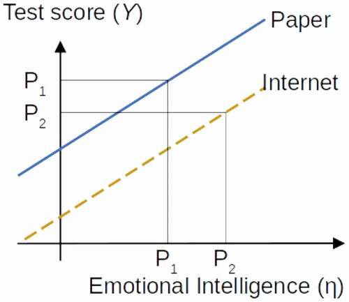
In contrast to full factorial invariance, item bias, also called partial factorial invariance (Millsap & Kwok, 2004), is present when two individuals with exactly the same standings on the latent constructs demonstrate different propensities to respond to one or more items. When measurement invariance does not hold for some items, meaning that item bias is present, the comparison of test scores across subpopulations is not valid and can be highly misleading. Consider the hypothetical example in Figure 1, where scalar invariance is violated for a test of emotional intelligence with respect to paper-and-pencil and Internet-based administrations. The overall bias, due to differences in the intercepts of the items, systematically leads to lower scores for persons using the Internet-based test. Therefore, Person 2, who has a higher true emotional intelligence level than Person 1 and takes the Internet-based test, gets a lower observed test score than Person 1, who takes the paper-and-pencil-based test.

Figure 1. Example of scalar non-invariance where a participant taking a paper test is mistakenly given a lower score.

An abundance of the previous literature has focused on statistical methods for detecting violations of factorial invariance, the most popular ones among which are the likelihood ratio test (LRT or ${\chi }^2$; Millsap, 2011) and the change in goodness-of-fit indices in structural equation modeling (Cheung & Rensvold, 2002). Using maximum likelihood estimation, a likelihood ratio ${\chi }^2$ statistic is obtained by comparing the maximized log-likelihoods of a model with invariance constraints (e.g., the metric invariance model with equality constraints on the factor loadings) and a model without such constraints (e.g., the configural invariance model without factor loading constraints). A significant test statistic then indicates that a particular step of measurement invariance is violated. However, the likelihood ratio test is very sensitive to large sample sizes such that items are flagged as noninvariant even when the degree of bias is trivial (Putnick & Bornstein, 2016). As an alternative, researchers rely on goodness-of-fit indices that are less sensitive to sample sizes, such as the comparative fit index (CFI; Bentler, 1990) and the root mean squared error of approximation (RMSEA; Steiger, 1980), and deem a psychological test practically invariant when the change in these indices is within a certain threshold (e.g., $\mathrm{\Delta }\mathrm{C}\mathrm{F}\mathrm{I}$ < .01 by Cheung & Rensvold, 2002; $\mathrm{\Delta }\mathrm{R}\mathrm{M}\mathrm{S}\mathrm{E}\mathrm{A}$ < .005 by Chen, 2007). These indices, however, are not meaningful metrics when it comes to communicating the degree of noninvariance of tests, as a $\mathrm{\Delta }$CFI of −.03, for example, does not indicate how using the test will be problematic in any concrete way.

Recently, there have been increased research efforts to define interpretable effect size indices for noninvariance at the item level. For example, Nye and Drasgow (2011) proposed the $d_{MACS}$ effect size, which corresponds to the expected standardized difference in observed item scores due to noninvariance; Nye et al. (2019) further provided benchmark values for $d_{MACS}$ based on a systematic review of the organizational literature. Gunn et al. (2020) proposed and evaluated several indices that are conceptually similar to $d_{MACS}$. However, because these indices focus on the impact of noninvariance on the item mean, they do not directly inform the impact on classification—a common usage of psychological tests—for two reasons. First, previous research usually assumes that biased items are automatically worse than unbiased items and, therefore, should be removed in order to achieve valid cross-group comparisons. However, while reducing bias in cross-group comparisons, removing biased items may make the test less reliable due to reduced test length, resulting in less precise inferences. When using test results for decision-making, both bias (systematic error) and precision (random error) should be taken into account. A slightly biased but highly effective item may contribute more information than an unbiased but ineffective item, but existing approaches for detecting item bias pays less attention to the role of unique variances and covariances (i.e., $\mathbf{\Theta }$), which is related to score reliability and is relevant to classification.¹

Second, as noted by Millsap and Kwok (2004), the evaluation of item bias should be made “in relation to the purpose of the measure” (pp. 94–95). In the behavioral sciences, a common purpose of a psychological test is to select or identify individuals based on their relative standings or absolute scores on the test (Crocker and Algina, 2006). Surprisingly, and unfortunately, very little attention has been paid to how noninvariance impacts selection. In the following section, we briefly review the relevant literature on item bias and classification, after which we define the MCAA framework as an extension to the approach by Millsap and Kwok (2004).

Factorial invariance in the context of selection

Psychological and behavioral measures are commonly used for various classification purposes: identifying people with depressive symptoms, selecting or promoting employees, and providing support for college admissions decisions. Often employers and test administrators compute a scale score or a composite score, denoted as $Z$, by applying a scoring rule on the item scores, such as by summing the items. The classification decisions are then based on $Z$.

As a hypothetical personnel selection example, imagine that two subgroups of applicants respond to a battery of assessment items (e.g., personality and cognitive tests). Without loss of generality, denote the two groups as the reference and the focal groups (Millsap & Kwok, 2004), where the focal group is considered to have a disadvantage due to potential measurement bias. Assume that the two groups are of equal sizes and have identical distributions on their actual, latent competency level. Based on their responses, each applicant receives a $Z$ score, and a manager wants to use the battery to select the top $10\mathrm{\%}$ of the combined pool of applicants. If the tests are bias-free, the final pool should consist of roughly $10\mathrm{\%}$ of participants from the reference group and $10\mathrm{\%}$ from the focal group, as shown in Figure 2a (i.e., the combined area of quadrants A and B). However, it is possible that due to noninvariance, or item bias, the reference group on average gets higher scores than the focal group. As a result and as shown in Figure 2b, $13.4\mathrm{\%}$ of the reference group but only $6.7\mathrm{\%}$ of the focal group are selected. In other words, the selection ratio changes from 1:1 to 2:1 between applicants in the reference and the focal groups.

Figure 2. Relationship between true latent construct scores (x-axis) and observed test scores (y-axis) for (a) a test with no item bias and (b) a test with biases against one subgroup. Quadrants A, B, C, and D indicates the proportions of true positives, false positives, true negatives, and false negatives.

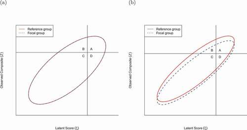
The example is simplified because it assumes an equal number of applicants from the focal and the reference groups with matched qualifications. Also, unless tests are perfectly reliable, some selected individuals in each subgroup will be “false positives;” a selection process that selects equal proportions of applicants in each subgroup is still problematic if it results in more false positives in some subgroups than others. A systematic approach to evaluating selection accuracy, as discussed in the remainder of the current paper, is needed to assess how factors, such as group sizes, differences in the distribution of qualifications, and reliability of the test scores may influence the effect of item bias on classification accuracy.

Classification accuracy analysis

Millsap and Kwok (2004) proposed a framework to quantify how noninvariance affects classification accuracy. Specifically, based on the probabilities of true positives (qualified and selected), false positives (unqualified but selected), true negatives (unqualified and not selected), and false negatives (qualified but not selected) (i.e., quadrants A, B, C, D in Figure 2), one can summarize classification accuracy by the following indices:

$\begin{array}{cc}\mathrm{P}\mathrm{r}\mathrm{o}\mathrm{p}\mathrm{o}\mathrm{r}\mathrm{t}\mathrm{i}\mathrm{o}\mathrm{n}\mathrm{s}\mathrm{e}\mathrm{l}\mathrm{e}\mathrm{c}\mathrm{t}\mathrm{e}\mathrm{d}(\mathrm{P}\mathrm{S})& =P(\mathrm{t}\mathrm{r}\mathrm{u}\mathrm{e}\mathrm{p}\mathrm{o}\mathrm{s}\mathrm{i}\mathrm{t}\mathrm{i}\mathrm{v}\mathrm{e})+P(\mathrm{f}\mathrm{a}\mathrm{l}\mathrm{s}\mathrm{e}\mathrm{p}\mathrm{o}\mathrm{s}\mathrm{i}\mathrm{t}\mathrm{i}\mathrm{v}\mathrm{e}),\\ \mathrm{S}\mathrm{u}\mathrm{c}\mathrm{c}\mathrm{e}\mathrm{s}\mathrm{s}\mathrm{R}\mathrm{a}\mathrm{t}\mathrm{i}\mathrm{o}(\mathrm{S}\mathrm{R})& =\frac{P(\mathrm{t}\mathrm{r}\mathrm{u}\mathrm{e}\mathrm{p}\mathrm{o}\mathrm{s}\mathrm{i}\mathrm{t}\mathrm{i}\mathrm{v}\mathrm{e})}{P(\mathrm{t}\mathrm{r}\mathrm{u}\mathrm{e}\mathrm{p}\mathrm{o}\mathrm{s}\mathrm{i}\mathrm{t}\mathrm{i}\mathrm{v}\mathrm{e})+P(\mathrm{f}\mathrm{a}\mathrm{l}\mathrm{s}\mathrm{e}\mathrm{p}\mathrm{o}\mathrm{s}\mathrm{i}\mathrm{t}\mathrm{i}\mathrm{v}\mathrm{e})},\\ \mathrm{S}\mathrm{e}\mathrm{n}\mathrm{s}\mathrm{i}\mathrm{t}\mathrm{i}\mathrm{v}\mathrm{i}\mathrm{t}\mathrm{y}(\mathrm{S}\mathrm{E})& =\frac{P(\mathrm{t}\mathrm{r}\mathrm{u}\mathrm{e}\mathrm{p}\mathrm{o}\mathrm{s}\mathrm{i}\mathrm{t}\mathrm{i}\mathrm{v}\mathrm{e})}{P(\mathrm{t}\mathrm{r}\mathrm{u}\mathrm{e}\mathrm{p}\mathrm{o}\mathrm{s}\mathrm{i}\mathrm{t}\mathrm{i}\mathrm{v}\mathrm{e})+P(\mathrm{f}\mathrm{a}\mathrm{l}\mathrm{s}\mathrm{e}\mathrm{n}\mathrm{e}\mathrm{g}\mathrm{a}\mathrm{t}\mathrm{i}\mathrm{v}\mathrm{e})},\\ \mathrm{S}\mathrm{p}\mathrm{e}\mathrm{c}\mathrm{i}\mathrm{f}\mathrm{i}\mathrm{c}\mathrm{i}\mathrm{t}\mathrm{y}(\mathrm{S}\mathrm{P})& =\frac{P(\mathrm{t}\mathrm{r}\mathrm{u}\mathrm{e}\mathrm{n}\mathrm{e}\mathrm{g}\mathrm{a}\mathrm{t}\mathrm{i}\mathrm{v}\mathrm{e})}{P(\mathrm{t}\mathrm{r}\mathrm{u}\mathrm{e}\mathrm{n}\mathrm{e}\mathrm{g}\mathrm{a}\mathrm{t}\mathrm{i}\mathrm{v}\mathrm{e})+P(\mathrm{f}\mathrm{a}\mathrm{l}\mathrm{s}\mathrm{e}\mathrm{p}\mathrm{o}\mathrm{s}\mathrm{i}\mathrm{t}\mathrm{i}\mathrm{v}\mathrm{e})},\end{array}$

where $P(\cdot )$ denotes the probability of an outcome.

For example, in personnel selection, proportion selected refers to the proportion of candidates selected for the job based on the biodata items. Success ratio is the proportion of candidates who are truly qualified among all the selected candidates; thus, a low success ratio means that the selection procedure selects many unqualified candidates for the job. Sensitivity is the proportion of candidates who are selected among all qualified candidates; thus, a low sensitivity means that only a small proportion of truly qualified candidates are selected. Finally, specificity is the proportion of candidates who are not selected among all the candidates who do not meet the cutoff, so a low specificity means that only a small proportion of truly unqualified candidates are correctly screened out. In this hypothetical example, one can argue that success ratio and sensitivity are more important if the goal is to select the best candidates, so proportion selected, success ratio, and sensitivity are important factors concerning the fairness of the selection procedure across subgroups. In practice, however, different combinations of these indices may matter most, depending on the purpose of the selection procedure.

The analyses originally proposed by Millsap and Kwok (2004) only computed PS, SR, SE, and SP. In the context of personnel selection, one additional index that is of interest is the adverse impact (AI) ratio, defined as (Nye & Drasgow, 2011)

$\mathrm{A}\mathrm{I}\mathrm{r}\mathrm{a}\mathrm{t}\mathrm{i}\mathrm{o}=\frac{{\mathrm{E}}_R(\mathrm{P}{\mathrm{S}}_F)}{\mathrm{P}{\mathrm{S}}_R},$

where $\mathrm{P}{\mathrm{S}}_R$ is the proportion selected for the reference group (usually the majority group), and ${\mathrm{E}}_R(\mathrm{P}{\mathrm{S}}_F)$ is the expected proportion selected for the focal group based on the latent score distributions of the reference group. In other words, ${\mathrm{E}}_R(\mathrm{P}{\mathrm{S}}_F)$ is the proportion that would be selected from the focal group when the focal and the reference groups were matched in latent trait levels. When strict invariance holds, the AI ratio is 1, meaning that two candidates with equal latent trait levels—one from the focal group and the other from the reference group—are equally likely to be selected. When AI ratio < 1, it indicates that those in the focal group would be less likely to be selected due to factors not related to the target latent traits.

To evaluate the impact of noninvariance on selection, researchers compute the classification accuracy indices based on the parameter estimates from a partial strict invariance model and a strict invariance model, respectively. They can then compare the two sets of classification accuracy indices, and holistically evaluate the impact of noninvariance on selection for each subpopulation.

Multidimensional classification accuracy analysis (MCAA) framework

Millsap and Kwok (2004)’s framework and follow-up research assumed unidimensionality of the items, meaning that all items used for selection measure one single latent trait. In actual personnel selection as well as in many classification tasks, the items may tap into multiple constructs, or constructs with multiple dimensions. For example, the Mini-International Personality Item Pool (Mini-IPIP; Donnellan et al., 2006), a personality inventory commonly used as part of personnel selection, has five dimensions (Openness, Conscientiousness, Extraversion, Agreeableness, and Neuroticism). Also, classification in practice may assign different weights to different dimensions, which means that individuals are selected based on a weighted composite score on the latent variables. Therefore, in this article, we propose a more general, multidimensional selection accuracy framework, and illustrate it using a secondary data analytic example.

For a selection test with $q$ dimensions, let ${\eta }_k$ be the true score for dimension $k$, and let $\mathbf{w}$ be a $1\times m$ row vector of weights. In other words, if we know the true, error-free score $\eta$ for every person, the selection should be based on $\varsigma =\mathbf{w}\eta$. However, we only have the error-prone scores on $p$ items, $\mathbf{y}$. Usually, the items can be similarly partitioned into $m$ subsets $[{\mathbf{y}{ }^{\mathrm{\prime }}}_1,{\mathbf{y}{ }^{\mathrm{\prime }}}_2,\dots ,{\mathbf{y}{ }^{\mathrm{\prime }}}_m]{ }^{\mathrm{\prime }}$, where each ${\mathbf{y}}_k$ component consists of $p_k$ items with ${\sum }_{k=1}^m{p}_k=p$. Let $\mathbf{c}=[c_1,c_2,\dots ,c_p]$ be the vector of weights for the items. So with only the item scores, the selection is based on $Z=\mathbf{c}\mathbf{y}$. Following the derivation in Millsap and Kwok (2004), under the multivariate normal assumption of $(\eta ,\epsilon )$, within each subpopulation $g$, $(Z_g,{\varsigma }_g)$ follows a bivariate normal distribution:

(2) $\left(\begin{array}{c}{Z}_g\\ {\varsigma }_g\end{array}\right)=N\left(\left[\begin{array}{c}\mathbf{c}{\nu }_g+\mathbf{c}{\mathbf{\Lambda }}_g{\alpha }_g\\ \mathbf{w}{\alpha }_g\end{array}\right],\left[\begin{array}{cc}\mathbf{c}{\mathbf{\Lambda }}_g{\mathbf{\Psi }}_g{\mathbf{\Lambda }{ }^{\mathrm{\prime }}}_g\mathbf{c}{ }^{\mathrm{\prime }}+\mathbf{c}{\mathbf{\Theta }}_g\mathbf{c}{ }^{\mathrm{\prime }}& \hspace{0.17em}\\ \mathbf{c}{\mathbf{\Lambda }}_g{\mathbf{\Psi }}_g\mathbf{w}{ }^{\mathrm{\prime }}& \mathbf{w}{\mathbf{\Psi }}_g\mathbf{w}{ }^{\mathrm{\prime }}\end{array}\right]\right),$(2)

and the marginal distribution of $(Z,\varsigma )$ is a finite mixture of bivariate normal distributions, with mixing proportions ${\pi }_1,\dots ,{\pi }_G$ based on the relative sizes of the subpopulations.

With a given cutscore on the observed composite, $Z_c$, and the total proportion selected, $\mathrm{P}{\mathrm{S}}_T=P(Z>Z_c)$, Millsap and Kwok (2004) showed that the cutscore on the latent composite, ${\varsigma }_c$, can be determined as the quantile in the mixture bivariate normal distribution corresponding to probability $\mathrm{P}{\mathrm{S}}_T$. Once $Z_c$ and ${\varsigma }_c$ are set, the classification accuracy indices for group $g$ can be easily obtained as cumulative probabilities in a bivariate normal distribution. We have created an R script with the major function PartInvMulti_we() (see the supplemental material) that automates the computation, so that users simply need to input the parameter values for each subpopulation, together with the mixing proportions and $Z_c$, to get the selection accuracy indices for each subpopulation. Below, we demonstrate the MCAA using real data of a personality inventory.

Comparing MCAA with the unidimensional counterpart

To demonstrate the need for a multidimensional framework, we conducted a simulation in which classification is based on two mildly correlated latent variables, and compared the classification accuracy indices based on MCAA as opposed to the unidimensional framework by Millsap and Kwok (2004). Specifically, we simulated 1,000 data sets, each with 10 items, where the first five items loaded on the first factor and the next five items loaded (primarily) on the second factor, with all loadings = .70; we also made item 10 to cross-load on the first factor with loading = .30. The items were fully metric invariant but three items were scalar noninvariant, with intercepts = 0 for all items in the first group and were 0.3, −0.1, and 0.5 for items 4, 5, and 10. Both latent factors had unity variance with a .2 correlation in both groups, and the unique variances were .51 for all items. We simulated 1,000 data sets, and for each data set, we obtained classification accuracy indices using MCAA with weights of $\mathbf{w}=[.7,.3]$ given to the two factors, respectively. The classification accuracy indices were based on selecting the top 25% on the latent composite. We also applied the unidimensional framework (as implemented in Lai et al., 2017) to obtain classification accuracy indices based on the first five items and the last five items separately, and obtained the weighted averages of the two sets of indices with the same weights of .7 and .3.

Table 1 compares the true population-level classification accuracy indices and the mean values across replications from MCAA and the unidimensional approach, with the first group as the reference group under partial strict invariance models. In summary, whereas MCAA recovered the true values of the indices well for both groups, using the unidimensional approach resulted in biased values of proportions selected and values of other indices being smaller than the true values.

Table 1. Simulation results

	Group 1				Group 2
	PS	SR	SE	SP	PS	SR	SE	SP
Population value	0.236	0.822	0.774	0.944	0.264	0.781	0.826	0.923
MCAA	0.236	0.821	0.774	0.944	0.264	0.780	0.826	0.923
UCAA	0.239	0.800	0.762	0.936	0.261	0.767	0.803	0.919

Note. UCAA = Unidimensional classification accuracy analysis applied separately to the two dimensions. PS = proportion selected. SR = success ration. SR = success ratio SE = sensitivity SP = specificity

Illustrative example

To illustrate the application of the multidimensional classification accuracy analysis (MCAA), we used data from Ock et al. (2020), which examined measurement invariance of the mini-IPIP across gender. The data are a subset of the Eugene-Springfield Community Sample collected from 1994 Spring to 1996 Fall (Goldberg, 2018), a well-studied community sample who completed a mail survey, including the mini-IPIP. Ock et al. (2020) performed listwise deletion and provided complete data in their supplemental material. The sample consisted of 564 participants (239 males, 325 females), who were 20–85 years old ($M$ = 51.7, $SD$ = 12.5), and nearly all of them being Caucasian ($97.7\mathrm{\%}$).

The mini-IPIP is a short form of the International Personality Item Pool, a personality measure based on the Five-Factor model (Donnellan et al., 2006; Goldberg, 1999). The mini-IPIP had 20 items in total, with four items for each factor. Specifically, items A2, A5, A7, A9 measure the factor Agreeableness; items C3, C4 C6, C8 measure the factor Conscientiousness; items E1, E4, E6, E7 measure the factor Extraversion; items N1, N2, N6, N8 measure the factor Neuroticism; and items O2, O8, O9, O10 measure the factor Openness to Experience. Further details about these items can be found in the Appendix in Donnellan et al. (2006). Questions were descriptive statements answered on a 5-point Likert-type scale from 1 (very inaccurate) to 5 (very accurate). Table 2 shows the means, standard deviations, and the correlations of the mini-IPIP items by gender.

Table 2. Mean, standard deviations, and item-level correlations of the mini-IPIP scales by gender

	Female		Male
	Mean	SD	Mean	SD	a2	a5	a7	a9	c3	c4	c8	c9	e1	e4	e6	e7	n1	n2	n6	n8	i2	i8	i9	i10
a2	4.34	0.73	3.93	0.87	1	.29	.18	.20	−.02	−.03	.10	.07	−.00	.06	.03	−.14	−.02	−.01	.06	−.03	−.01	.01	−.04	.01
a5	4.07	0.84	3.53	1.02	.51	1	.33	.39	.04	−.10	.02	−.06	.12	.20	.13	.05	−.08	.00	.09	−.02	.19	.11	.14	.14
a7	4.45	0.83	4.04	0.90	.30	.45	1	.44	−.02	−.12	.14	.06	.08	.19	.08	.04	−.07	−.14	−.08	−.13	.13	.11	.13	.15
a9	4.18	0.82	3.61	0.96	.32	.51	.56	1	−.01	−.13	.03	−.03	.01	.09	.00	.01	−.12	−.06	−.08	−.13	.06	.05	.07	.09
c3	3.37	1.22	3.28	1.09	.06	.08	.10	.01	1	.31	.31	.39	.05	.05	−.02	−.01	−.07	−.12	−.04	−.17	−.11	−.01	−.10	−.00
c4	4.32	0.77	4.26	0.71	.04	−.01	.04	−.06	.22	1	.20	.35	.02	−.05	.00	.06	.10	−.07	.05	−.03	−.10	−.10	−.08	−.12
c8	4.23	0.97	4.18	0.81	.05	−.03	.09	.05	.21	.27	1	.33	.13	.13	.07	.13	−.02	−.20	−.10	−.26	−.12	.01	−.04	−.05
c9	3.70	1.32	3.61	1.22	.00	.01	−.01	−.13	.32	.41	.30	1	.04	.05	−.01	.01	−.03	−.13	−.04	−.10	−.05	.07	.02	−.03
e1	2.22	1.15	2.31	1.03	.11	.16	.10	.11	.01	−.08	−.10	.03	1	.38	.37	.40	−.11	−.11	.04	−.03	.14	.10	.14	.15
e4	2.94	1.30	2.88	1.24	.04	.18	.25	.16	.13	.02	.02	.10	.41	1	.38	.34	−.07	−.11	.00	−.09	.10	.08	.06	.17
e6	3.41	1.24	3.01	1.21	.12	.19	.34	.29	−.12	−.08	−.01	−.01	.35	.40	1	.39	.01	−.03	.05	−.09	.14	.11	.18	.19
e7	3.08	1.02	3.09	1.08	.07	.06	.18	.12	.07	−.03	.10	−.00	.42	.35	.48	1	−.06	−.22	−.02	−.16	.07	.07	.12	.17
n1	2.54	1.11	2.26	0.97	−.15	−.05	.00	.05	−.04	−.02	−.10	.06	.09	−.03	.11	.04	1	.27	.37	.33	−.07	.09	.02	−.10
n2	2.66	1.32	2.46	1.12	−.24	−.08	−.15	−.09	−.09	.02	−.17	−.03	−.02	−.12	−.01	−.06	.41	1	.41	.49	−.04	.04	−.02	−.10
n6	2.31	1.08	2.30	1.05	−.19	−.09	−.14	−.14	−.13	.04	−.18	−.02	.08	−.03	.12	−.01	.31	.40	1	.41	.00	−.04	−.04	−.03
n8	2.23	1.20	2.29	1.15	−.14	−.03	−.09	−.12	−.12	−.00	−.23	.01	−.05	−.11	.01	−.04	.39	.54	.41	1	.08	.06	.02	−.02
i2	3.76	1.13	3.94	0.97	.08	.15	.21	.13	−.02	.02	−.06	.00	.26	.17	.31	.25	−.00	.02	.03	.09	1	.26	.32	.63
i8	3.35	1.26	3.65	1.13	.10	.02	.08	.11	.01	−.07	.06	−.06	.09	.19	.22	.28	.02	−.03	−.14	−.08	.23	1	.65	.24
i9	3.38	1.23	3.62	1.09	.17	.17	.19	.32	−.06	−.02	−.01	−.13	.08	.14	.21	.16	−.00	.01	−.15	−.00	.26	.50	1	.34
i10	3.81	1.18	4.07	1.05	.06	.08	.20	.14	.05	.07	.02	.03	.22	.17	.26	.27	.00	−.04	−.12	−.02	.57	.32	.26	1

Note. The item-level correlations of males (females) are shown in the lower (upper) triangle.

To identify noninvariant parameters, we used the lavaan R package (Rosseel, 2012) and the forward specification search procedure (Yoon & Kim, 2014) using likelihood ratio tests ($\mathrm{\Delta }{\chi }^2$).² Given the categorical nature of the items, we followed Ock et al. (2020) to use the robust maximum likelihood (MLR) estimator, with the scaled $\mathrm{\Delta }{\chi }^2$ test by Satorra and Bentler (2001). We first fitted a configural invariance model, which showed poor fit, ${\chi }^2(320)=662.94$, $p<.001$, RMSEA = 0.06, 95%CI [0.06, 0.07], CFI = 0.84, SRMR = 0.06. Based on the modification indices, we decided to free eight pairs of unique factor covariances: A2 and A5, E4 and E7, I2 and I10, I8 and I9, A9 and I9, C3 and E6, A2 and E7, E7 and N2. The modified configural invariance model with five factors (see Figure 3) showed acceptable fit, ${\chi }^2(304)=408.96$, $p<.001$, RMSEA = 0.03, 95%CI [0.03, 0.04], CFI = 0.95, SRMR = 0.05. Equality constraints in the loadings did not result in poorer model fit, scaled $\mathrm{\Delta }{\chi }^2(15)=10.83$, $p=.764$. We then added the constraints to the intercepts, which resulted in poorer model fit, scaled $\mathrm{\Delta }{\chi }^2(15)=49.38$, $p<.001$. One item in Agreeableness (A2, “Sympathize with others’ feelings”), one item in Extraversion (E6 “Don’t talk a lot”) and two items in Neuroticism (N1, “Am relaxed most of the time”; N2, “Seldom feel blue”) showed noninvariant intercepts across groups ($\mathrm{\Delta }{\nu }_{\mathrm{F}-\mathrm{M}}$ = 0.16, 0.42, 0.31, 0.24). After freeing these items, the scalar model showed acceptable fit, ${\chi }^2(330)=426.75$, $p<.001$, RMSEA = 0.03, 95%CI [0.02, 0.04], CFI = 0.95, SRMR = 0.05. A strict invariance model was further fitted to the data, which fitted the data worse than the partial scalar invariance model, scaled ${\mathrm{\Delta }}^2\chi (20)=40.65$, $p=.004$. One item in Conscientiousness (C8, “Make a mess of things”) and two items in Neuroticism (N1, “Am relaxed most of the time”; N2, “Seldom feel blue”) showed noninvariant unique factor variance across groups ($\mathrm{\Delta }{\theta }_{\mathrm{F}-\mathrm{M}}$ = 0.21, 0.28, 0.39). The final model is a partial strict invariance model, ${\chi }^2(347)=446.25$, $p<.001$, RMSEA = 0.03, 95%CI [0.02, 0.04], CFI = 0.95, SRMR = 0.06. The parameter estimates from the partial strict invariance model can be found in the supplemental material.

Figure 3. Path diagram of the factor model for the mini-IPIP items in the illustrative example.

While the conventional invariance testing identified four items with noninvariant intercepts, the results did not provide information on how these noninvariant parameters may impact personnel selection using the mini-IPIP. For example, do the noninvariant intercepts give a substantial or a negligible advantage to females? Does dropping the noninvariant items improve the selection procedure? To answer these questions, we show how MCAA can be applied in a step-by-step fashion.

Step 1: Selection parameters

As a first step of doing MCAA, we need to consider several parameters related to selection: (a) the mixing proportion (${\pi }_g$), (b) the relative weights given to each dimension ($w_k$), (c) the weights given to each item ($c_j$), and (d) the selection cutoff, either in terms of an absolute cutoff score ($Z_c$) or a relative cutoff proportion (i.e. proportion selected). In this example, because the population sizes for females and for males are roughly equal, we use ${\pi }_1={\pi }_2=.5$. The weights given to the items and to the different dimensions require some more considerations. If the test items are summed together to get one single scale score for selection purposes, and each dimension contains an equal number of items, then we can specify $\mathbf{w}=\mathbf{1}$ (i.e., a vector of ones). However, it is well documented in previous research (e.g., Barrick & Mount, 1991) that different personality dimensions had different associations with job performance. Instead, we used the regression weights reported by Drasgow et al. (2012), which conducted a meta-analysis to examine the predictive validity of five personality dimensions in eight criteria of job performance (e.g., the predictive validity of conscientiousness ranges from −0.23 to 0.20). After averaging the regression weights for each dimension, we set $\mathbf{w}=[.0325,.1795,.4693,-.1951,.1236]$ for agreeableness, conscientiousness, extraversion, neuroticism (with a negative weight), and openness. Note that the sum of the absolute values of the weights is one. On the item side, because each dimension has the same number of items, we set the item weights to be proportional to the latent weights, while keeping the maximum weighted score for each participant to 100 (same as the unweighted score); specifically, $\mathbf{c}=5\times [w_1,w_1,w_1,w_1,\dots ,w_5,w_5,w_5,w_5]$ for 20 items. The codes for obtaining the weights can be found in the supplemental material. For the selection cutoff, we assume that the mini-IPIP is used to select the top 25% of the candidates.

Step 2: Classification accuracy under strict invariance

To establish the baseline information of using the mini-IPIP in selecting males and females, we first obtained the parameter estimates under full strict invariance. The supplemental material contains codes for extracting parameter estimates from a fitted lavaan model object as inputs for the MCAA; however, researchers can also manually input the parameter estimates into the provided R function, PartInvMulti_we(). Following Millsap and Kwok (2004), for the four noninvariant intercepts and the three noninvariant unique factor variances, we obtained the average parameter estimates weighted by the mixing proportions as parameters for the strict invariance model. We used female candidates as the reference group and male candidates as the focal group. Using the selection parameters in Step 1 and the R script in the supplemental material, one can obtain the selection indices when strict invariance holds, as shown in Table 3. Specifically, the selection is expected to comprise slightly more female candidates (25.2%) than male candidates. The other classification accuracy indices (success ratio, sensitivity, and specificity) were similar for the two groups.

Table 3. Impact of item bias on selection accuracy indices from the multidimensional classification accuracy analysis

	Strict Invariance			Partial Strict Invariance
	Female	Male	${\mathrm{E}}_F(\mathrm{M}\mathrm{a}\mathrm{l}\mathrm{e})$	Female	Male	${\mathrm{E}}_F(\mathrm{M}\mathrm{a}\mathrm{l}\mathrm{e})$
Proportion selected	0.252	0.248	0.252	0.260	0.240	0.243
Success ratio	0.748	0.743	0.748	0.732	0.759	0.764
Sensitivity	0.749	0.742	0.749	0.758	0.733	0.739
Specificity	0.915	0.915	0.915	0.907	0.923	0.923

Note. The column ${\mathrm{E}}_F(\mathrm{M}\mathrm{a}\mathrm{l}\mathrm{e})$ shows the expected values for male candidates using the latent distributions of female candidates.

Step 3: Classification accuracy under partial strict invariance

The selection accuracy of mini-IPIP under partial strict invariance can be obtained in the same way as in Step 2, except that the intercept parameters were different for males and females, as well as the unique variances and covariances. The results are again shown in Table 3. In the presence of test bias, male candidates are selected in a lower proportion than female candidates (0.260 for female and 0.240 for male). The selection procedure has a higher sensitivity for female than male candidates (0.758 for female and 0.733 for male). However, female candidates have a lower success ratio (0.732 for female and 0.759 for male) and specificity (0.907 for female and 0.923 for male) than male candidates.

Step 4: Compare the change in classification accuracy indices

Comparing the results in Steps 2 and 3, we see male candidates are selected in a lower proportion (24.0%), whereas female candidates are selected in a higher proportion (26.0%). The increased proportion selected for female candidates due to item bias, however, results in a lower success ratio (0.732 as opposed to 0.748 under strict invariance), meaning that there are more false positives among qualified female candidates. Item bias also results in a higher sensitivity (0.758 as opposed to 0.749) and a lower specificity (0.907 as opposed to 0.915) for females. On the contrary, the lower proportion selected for male candidates results in a higher success ratio (0.759 as opposed to 0.743), lower sensitivity (0.733 as opposed to 0.742), and higher specificity (0.923 as opposed to 0.915).

The columns labeled $E_F(\mathrm{M}\mathrm{a}\mathrm{l}\mathrm{e})$ in Table 3 represent the expected classification performance for male candidates based on the latent score distributions of the female candidates. The differences between columns $\mathrm{F}\mathrm{e}\mathrm{m}\mathrm{a}\mathrm{l}\mathrm{e}$ and $E_F(\mathrm{M}\mathrm{a}\mathrm{l}\mathrm{e})$ show the impact of item bias on classification accuracy, as they are identical when strict invariance holds. Our R function also computed the AI ratio for male candidates to be 0.935, which is the ratio of proportions selected for females and the proportions selected for $E_F(\mathrm{M}\mathrm{a}\mathrm{l}\mathrm{e})$ under strict invariance, that is, .243/.260. The computed AI ratio indicates that, due to item bias, for every 1,000 female candidates selected, only 935 equally qualified male candidates will be selected. Thus, it demonstrates a disadvantage for male candidates when using the mini-IPIP for selection.

Comparison with separate unidimensional analyses

We also applied separate unidimensional analysis to each dimension of the mini-IPIP. Because Agreeableness, Conscientiousness, and Openness were not found to show partial invariance when evaluated separately, only the results of Extraversion and Neuroticism are reported in Table 4.³ Note that the results for Neuroticism were based on reversely coded items, as lower neuroticism is usually preferred in personnel selection. It can be seen that the impact of item bias on selection accuracy is larger when considering each dimension separately than the combined impacts obtained from MCAA. Consider selecting individuals solely based on extraversion. Under strict invariance, female candidates will be selected at a similar proportion (24.7%) as male candidates (25.3%), but more females will be selected (26.7%) under partial strict invariance. The reverse is true for Neuroticism, as more males will be selected under partial strict invariance. The item biases showed a particularly large impact on sensitivity. However, when considering the combined effect of item biases across all dimensions, as shown by MCAA, the impact was much smaller, as the biases in Extraversion and in Neuroticism somewhat canceled out. The sensitivity and specificity also had higher values under MCAA, as the selection was generally more accurate with 20 items from five dimensions as opposed to only 4 items in one dimension. Therefore, when a multidimensional test is used for selection or classification purposes, using the MCAA framework provides results more closely aligned to how item biases affect the actual classification decisions overall.

Table 4. Impact of item bias on selection accuracy indices when the dimensions are considered separately

	Strict Invariance		Partial Strict Invariance
	Female	Male	Female	Male
Extraversion
Proportion selected	0.247	0.253	0.267	0.233
Success ratio	0.714	0.715	0.691	0.738
Sensitivity	0.715	0.714	0.748	0.680
Specificity	0.906	0.903	0.891	0.918
Neuroticism (Reverse coded)
Proportion selected	0.261	0.239	0.238	0.262
Success ratio	0.741	0.708	0.756	0.693
Sensitivity	0.734	0.717	0.683	0.768
Specificity	0.908	0.909	0.921	0.895

Discussion

Despite tremendous growth in the measurement invariance literature, there has been a disconnect between how results of invariance testing are presented – usually in the form of statistical significance and change in fit indices – and how psychological measures are used in practice for making classification decisions. The work by Millsap and Kwok (2004) and Stark et al. (2004) provided a foundation for understanding the impact of noninvariance on classification. Nevertheless, the previous work only considered unidimensional items, but in practice, classification is usually done based on multiple dimensions.

The current work proposes a multidimensional classification accuracy framework (MCAA), which examines the change in classification accuracy indices attributable to noninvariance across demographic subgroups. We conceptualize the multidimensional problem by considering the joint distribution of the weighted observed composite score and the weighted latent composite score, and provide software code that computes the change in classification accuracy indices due to noninvariance. We illustrate MCAA with a step-by-step example of a five-dimensional personality inventory commonly used for personnel selection.

Readers should note that the MCAA and the foundational work by Millsap and Kwok (2004) only represent one option for understanding the practical significance of noninvariance. Other effect size indices exist in the literature, some of which were nicely summarized in Meade (2010), and some recent development was made by Nye et al. (2019) and Gunn et al. (2020). In our opinion, information on changes in classification accuracy indices is most relevant for measures that are potentially used for classification purposes, such as tests of cognitive and noncognitive abilities, as well as screening and diagnostic tools. When conducting invariance analysis, we encourage researchers to carefully consider the intended usage of the measure being studied and report the magnitude of noninvariance (if any) in a metric that is easily interpretable and fits the context in which the measure will be used.

While we think the MCAA represents a step closer to linking invariance research and actual practices in the context of classification, we also recognize some limitations of the current work and encourage future research efforts to address them. First, the current framework assumes that item responses are approximately continuous; given that binary and ordinal items are commonly used in psychological measures, future research can combine MCAA and the recent extension by Gonzalez and Pelham (2021) and Lai et al. (2019). Second, as with previous literature, the implied classification accuracy indices under the strict and the partial strict invariance models are only point estimates and are subject to sampling error. Given the recommendations on reporting uncertainty estimates for measures on practical significance (e.g., American Psychological Association, 2020), future work is needed to develop methods for obtaining standard errors and confidence intervals for the classification accuracy indices.

Disclosure statement

No potential conflict of interest was reported by the author(s).

Additional information

Funding

This work was supported by the the U.S. Army Research Institute for the Behavioral and Social Sciences (ARI) [W911NF-20-1-0282].

Notes

¹ An example of this can be found in the supplemental material, where selection drops after deleting five noninvariant items in a 20-item test.

² Jung and Yoon (2016) and Jung and Yoon (2017) are accessible introductions to other methods for identifying non-invariant parameters.

³ Evaluating measurement invariance for each dimension, we found one item for Extraversion (E6 “Don’t talk a lot”) had noninvariant intercepts, and two items in Neuroticism (N1, “Am relaxed most of the time”; N2, “Seldom feel blue”) had noninvariant intercepts and unique variances across gender.

References

- Aguinis, H., Culpepper, S. A., & Pierce, C. A. (2016). Differential prediction generalization in college admissions testing. Journal of Educational Psychology, 108, 1045–1059. https://doi.org/https://doi.org/10.1037/edu0000104
- American Educational Research Association, American Psychological Association, & National Council on Measurement in Education. (2014). Standards for educational and psychological testing. https://www.testingstandards.net/open-access-files.html
- American Psychological Association. (2020). Publication manual of the American Psychological Association (7th ed.). https://doi.org/https://doi.org/10.1037/000016S-000
- Barrick, M. R., & Mount, M. K. (1991). The Big Five personality dimensions and job performance: A meta-analysis. Personnel Psychology, 44, 1–26. https://doi.org/https://doi.org/10.1111/j.1744-6570.1991.tb00688.x
- Bentler, P. M. (1990). Comparative fit indexes in structural models. Psychological Bulletin, 107, 238–246. https://doi.org/https://doi.org/10.1037/0033-2909.107.2.238
- Chen, F. F. (2007). Sensitivity of goodness of fit indices to lack of measurement invariance. Structural Equation Modeling: A Multidisciplinary Journal, 14, 464–504. https://doi.org/https://doi.org/10.1080/10705510701301834
- Cheung, G. W., & Rensvold, R. B. (2002). Evaluating goodness-of-fit indexes for testing measurement invariance. Structural Equation Modeling: A Multidisciplinary Journal, 9, 233–255. https://doi.org/https://doi.org/10.1207/S15328007SEM0902_5
- Crocker, L.M., and Algina, J. (2006). Introduction to classical and modern test theory. Cengage Learning.
- Donnellan, M., Oswald, F., Baird, B., & Lucas, R. (2006). The Mini-IPIP scales: Tiny-yet-effective measures of the big five factors of personality. Psychological Assessment, 18, 192–203. https://doi.org/https://doi.org/10.1037/1040-3590.18.2.192
- Drasgow, F., Stark, S., Chernyshenko, O. S., Nye, C. D., Hulin, C. L., & White, L. A. (2012). Development of the Tailored Adaptive Personality Assessment System (TAPAS) to support Army personnel selection and classification decisions (Technical Report 1311). U.S. Army Research Institute for the Behavioral and Social Sciences. https://apps.dtic.mil/sti/citations/ADA564422
- Goldberg, L. R. (2018). (2,8,10 & others) International Personality Item Pool (IPIP) (Version V1) [Data set]. Harvard Dataverse. https://doi.org/https://doi.org/10.7910/DVN/UF52WY
- Goldberg, L. R. (1999). A broad-bandwidth, public domain, personality inventory measuring the lower-level facets of several five-factor models. In I. Mervielde, I. J. Deary, F. De Fruyt, & F. Ostendorf (Eds.),Personality Psychology in Europe, 7, 7–28. Tilburg University Press.
- Gonzalez, O., & Pelham, W. E. (2021). When does differential item functioning matter for screening? A method for empirical evaluation. Assessment, 28, 446–456. https://doi.org/https://doi.org/10.1177/1073191120913618
- Gunn, H. J., Grimm, K. J., & Edwards, M. C. (2020). Evaluation of six effect size measures of measurement non-Invariance for continuous outcomes. Structural Equation Modeling: A Multidisciplinary Journal, 27, 503–514. https://doi.org/https://doi.org/10.1080/10705511.2019.1689507
- Horn, J. L., & Mcardle, J. J. (1992). A practical and theoretical guide to measurement invariance in aging research. Experimental Aging Research, 18, 117–144. https://doi.org/https://doi.org/10.1080/03610739208253916
- Hurtz, G. M., & Donovan, J. J. (2000). Personality and job performance: The big five revisited. Journal of Applied Psychology, 85, 869–879. https://doi.org/https://doi.org/10.1037/0021-9010.85.6.869
- Jung, E., & Yoon, M. (2016). Comparisons of three empirical methods for partial factorial invariance: Forward, backward, and factor-ratio tests. Structural Equation Modeling: A Multidisciplinary Journal, 23, 567–584. https://doi.org/https://doi.org/10.1080/10705511.2015.1138092
- Jung, E., & Yoon, M. (2017). Two-step approach to partial factorial invariance: Selecting a reference variable and identifying the source of noninvariance. Structural Equation Modeling: A Multidisciplinary Journal, 24, 65–79. https://doi.org/https://doi.org/10.1080/10705511.2016.1251845
- Lai, M. H. C., Kwok, O.-M., Yoon, M., & Hsiao, -Y.-Y. (2017). Understanding the impact of partial factorial invariance on selection accuracy: An R script. Structural Equation Modeling: A Multidisciplinary Journal, 24, 783–799. https://doi.org/https://doi.org/10.1080/10705511.2017.1318703
- Lai, M. H. C., Richardson, G. B., & Mak, H. W. (2019). Quantifying the impact of partial measurement invariance in diagnostic research: An application to addiction research. Addictive Behaviors, 94, 50–56. https://doi.org/https://doi.org/10.1016/j.addbeh.2018.11.029
- Meade, A. W. (2010). A taxonomy of effect size measures for the differential functioning of items and scales. Journal of Applied Psychology, 95, 728–743. https://doi.org/https://doi.org/10.1037/a0018966
- Mellenbergh, G. J. (1989). Item bias and item response theory. International Journal of Educational Research, 13, 127–143. https://doi.org/https://doi.org/10.1016/0883-0355(89)90002-5
- Meredith, W. (1993). Measurement invariance, factor analysis and factorial invariance. Psychometrika, 58, 525–543. https://doi.org/https://doi.org/10.1007/BF02294825
- Millsap, R. E., & Kwok, O.-M. (2004). Evaluating the impact of partial factorial invariance on selection in two populations. Psychological Methods, 9, 93–115. https://doi.org/https://doi.org/10.1037/1082-989X.9.1.93
- Millsap, R. E. (2007). Invariance in measurement and prediction revisited. Psychometrika, 72, 461–473. https://doi.org/https://doi.org/10.1007/s11336-007-9039-7
- Millsap, R. E. (2011). Statistical approaches to measurement invariance. Routledge.
- Nye, C. D., Bradburn, J., Olenick, J., Bialko, C., & Drasgow, F. (2019). How big are my effects? examining the magnitude of effect sizes in studies of measurement equivalence. Organizational Research Methods, 22, 678–709. https://doi.org/https://doi.org/10.1177/1094428118761122
- Nye, C. D., & Drasgow, F. (2011). Effect size indices for analyses of measurement equivalence: Understanding the practical importance of differences between groups. Journal of Applied Psychology, 96, 966–980. https://doi.org/https://doi.org/10.1037/a0022955
- Ock, J., McAbee, S. T., Mulfinger, E., & Oswald, F. L. (2020). The practical effects of measurement invariance: Gender invariance in two Big Five personality measures. Assessment, 27, 657–674. https://doi.org/https://doi.org/10.1177/1073191119885018
- Putnick, D. L., & Bornstein, M. H. (2016). Measurement invariance conventions and reporting: The state of the art and future directions for psychological research. Developmental Review, 41, 71–90. https://doi.org/https://doi.org/10.1016/j.dr.2016.06.004
- Rosseel, Y. (2012). lavaan: An R package for structural equation modeling. Journal of Statistical Software, 48, 1–36. https://doi.org/https://doi.org/10.18637/jss.v048.i02
- Satorra, A., & Bentler, P. M. (2001). A scaled difference chi-square test statistic for moment structure analysis. Psychometrika, 66, 507–514. https://doi.org/https://doi.org/10.1007/BF02296192
- Schmidt, F. L., & Hunter, J. E. (1998). The validity and utility of selection methods in personnel psychology: Practical and theoretical implications of 85 years of research findings. Psychological Bulletin, 124, 262–274. https://doi.org/https://doi.org/10.1037/0033-2909.124.2.262
- Schmit, M. J., & Ryan, A. M. (1993). The Big Five in personnel selection: Factor structure in applicant and nonapplicant populations. Journal of Applied Psychology, 78, 966–974. https://doi.org/https://doi.org/10.1037/0021-9010.78.6.966
- Schmitt, N., & Kuljanin, G. (2008). Measurement invariance: Review of practice and implications. Human Resource Management Review, 18, 210–222. https://doi.org/https://doi.org/10.1016/j.hrmr.2008.03.003
- Stark, S., Chernyshenko, O. S., & Drasgow, F. (2004). Examining the effects of differential item (functioning and differential) test functioning on selection decisions: When are statistically significant effects practically important? Journal of Applied Psychology, 89, 497–508. https://doi.org/https://doi.org/10.1037/0021-9010.89.3.497
- Steiger, J. H. (1980). Statistically-based tests for the number of common factors. Paper presented at the annual meeting of the Psychometric Society. Iowa City, IA. Retrieved March 8, 2021, from https://ci.nii.ac.jp/naid/10012870999/
- Thurstone, L. L. (1947). Multiple factor analysis. University of Chicago Press.
- Vandenberg, R. J. (2002). Toward a further understanding of and improvement in measurement invariance methods and procedures. Organizational Research Methods, 5, 139–158. https://doi.org/https://doi.org/10.1177/1094428102005002001
- Yoon, M., & Kim, E. S. (2014). A comparison of sequential and nonsequential specification searches in testing factorial invariance. Behavior Research Methods, 46, 1199–1206. https://doi.org/https://doi.org/10.3758/s13428-013-0430-2
- Zwick, R., Thayer, D. T., & Lewis, C. (1999). An empirical Bayes approach to Mantel-Haenszel DIF analysis. Journal of Educational Measurement, 36, 1–28. https://doi.org/https://doi.org/10.1111/j.1745-3984.1999.tb00543.x