Caught off Base: A Note on the Interpretation of Incremental Fit Indices

Abstract

This note serves as a reminder that incremental fit indices are a form of standardized effect sizes and hence, all reservations with respect to interpretations of standardized effect sizes also transfer to their interpretation. Such a realization has major implications for the interpretation and use of incremental fit indices, for the theoretical (im)possibility of default universal rules of thumb in their application, and for simulation studies mapping incremental fit indices as if their value is comparable in an absolute sense across any and all conditions. A small but illustrative working example centered around the alleged impact of model type will drive these points home.

Keywords:

• Baseline model
• determinant
• incremental fit index
• model type
• relative model fit

Model fit assessment and model comparison remain universally important but also confusing topics in structural equation modeling (SEM). Tons of model fit tests and diagnostic fit indices have been introduced for purpose of model fit assessment—with Marsh et al. for instance already looking at 29 fit indices early on in 1988 —and new developments are abundant and extend fit indices beyond their initial boundaries (e.g., non-normal data, bias-reduction; see for example Raykov, 2005; Yuan & Bentler, 2000). Recent practice has arguably converged to reporting multiple fit indices and following rules of thumb based on the work by Hu and Bentler (1999), with the chisquare statistic (${\chi }^2$), Root Mean Square Error of Approximation (RMSEA), and Comparative Fit Index (CFI) among the popular indices to use and report (Jackson et al., 2009). For model assessment guidelines and rules of thumb for fit indices to work, they should be proven to function rather universally across a broad scope of data and model characteristics. Yet, the extensive simulation literature on this matter has already put forward many factors that are influencing the general applicability of the rules of thumb (for a review, see e.g., Niemand & Mai, 2018) leading to a general caution on their universality.

This general caution is also readily ignored in practice where a binary search for adherence with the rules of thumb for a range of fit indices is the factual norm. The latter might come across as a surprise but is in line with McDonald and Ho (2002) who state that “it is sometimes suggested that we should report a large number of these indices, apparently because we do not know how to use any of them” (p. 72), resulting in a lack of deliberate decision making. To make more informed decisions with respect to the use of fit indices it is important to know how these fit indices work. However, as Lai and Green (2016) point out “the meaning of ‘good’ fit and how it relates to fit indices are not well-understood in the current literature” (p. 234).

This manuscript sets out to remind/clarify what the meaning of good fit is for incremental fit indices and what implications this should have for their use in practice. The alleged impact of model type on incremental fit indices is used as a working example to elucidate the actual impact of the baseline as opposed to the type of target model.

1. Incremental Fit Indices

Incremental fit indices, such as the Normed Fit Index (NFI: Bentler & Bonett, 1980), Comparative Fit Index (CFI: Bentler, 1990), or Tucker-Lewis Index (TLI: Tucker & Lewis, 1973) are part of a family of relative fit measures for structural equation modeling that involves locating a model of interest within a continuum of models from the worst fitting baseline model to the perfect fitting or saturated model. Incremental fit indices are much like SEM counterparts of r-square indices in linear regression. (1) $$\begin{array}{ccc}{r}_{Y|\mathbf{X}}^2& =& \mathrm{\backslash !}\mathrm{\backslash !}\mathrm{\backslash !}\mathrm{\backslash !}\mathrm{\backslash !}\mathrm{\backslash !}\mathrm{\backslash !}\mathrm{\backslash !}\mathrm{\backslash !}\mathrm{\backslash !}\mathrm{\backslash !}\mathrm{\backslash !}\mathrm{\backslash !}\mathrm{\backslash !}\mathrm{\backslash !}\mathrm{\backslash !}\mathrm{\backslash !}\mathrm{\backslash !}\mathrm{\backslash !}\mathrm{\backslash !}\mathrm{\backslash !}\mathrm{\backslash !}\mathrm{\backslash !}\mathrm{\backslash !}\mathrm{\backslash !}\mathrm{\backslash !}\mathrm{\backslash !}\mathrm{\backslash !}\mathrm{\backslash !}\mathrm{\backslash !}\mathrm{\backslash !}1-\frac{S{S}_{\mathit{error}}}{S{S}_{\mathit{total}}}\\ {\text{NFI}}_{(m,b)}& =& \mathrm{\backslash !}\mathrm{\backslash !}\mathrm{\backslash !}\mathrm{\backslash !}\mathrm{\backslash !}\mathrm{\backslash !}\mathrm{\backslash !}\mathrm{\backslash !}\mathrm{\backslash !}\mathrm{\backslash !}\mathrm{\backslash !}\mathrm{\backslash !}\mathrm{\backslash !}\mathrm{\backslash !}\mathrm{\backslash !}\mathrm{\backslash !}\mathrm{\backslash !}\mathrm{\backslash !}\mathrm{\backslash !}\mathrm{\backslash !}\mathrm{\backslash !}\mathrm{\backslash !}\mathrm{\backslash !}\mathrm{\backslash !}\mathrm{\backslash !}\mathrm{\backslash !}\mathrm{\backslash !}\mathrm{\backslash !}\mathrm{\backslash !}\mathrm{\backslash !}\mathrm{\backslash !}\mathrm{\backslash !}\mathrm{\backslash !}\mathrm{\backslash !}\mathrm{\backslash !}\mathrm{\backslash !}\mathrm{\backslash !}\mathrm{\backslash !}1-\frac{{\chi }_m^2}{{\chi }_b^2}\\ {\text{CFI}}_{(m,b)}& =& 1-\frac{{\lambda }_m}{{\lambda }_b}=1-\frac{{\chi }_m^2-{\text{df}}_m}{{\chi }_b^2-{\text{df}}_b}\\ {\text{TLI}}_{(m,b)}& =& \mathrm{\backslash !}\mathrm{\backslash !}\mathrm{\backslash !}\mathrm{\backslash !}\mathrm{\backslash !}\mathrm{\backslash !}\mathrm{\backslash !}\mathrm{\backslash !}\mathrm{\backslash !}\mathrm{\backslash !}\mathrm{\backslash !}\mathrm{\backslash !}\frac{{\chi }_b^2/{\text{df}}_b-{\chi }_m^2/{\text{df}}_m}{{\chi }_b^2/{\text{df}}_b-1}\\ \text{effect}\mathrm{ }\text{size}& =& 1-\frac{\text{misspecification}\mathrm{ }\text{of}\mathrm{ }\text{target}\mathrm{ }\text{model }‘\text{m}’\text{vs}\mathrm{ }\text{saturated}\mathrm{ }\text{model}}{\text{misspecification}\mathrm{ }\text{baselinemodel}\mathrm{ }‘\text{b}’\text{vs}\mathrm{ }\text{saturated}\mathrm{ }\text{model}}\end{array}$$(1)

Note. $r_{Y|\mathbf{X}}^2$ = r-squared, relative reduction in prediction error of Y given predictors X; SS_error = error sum of squares, sum of squared differences between each data point y_i and their estimated value ${\widehat{y}}_i;$ SS_total = total sum of squares, sum of squared differences between each data point y_i and the average $\overline{y};$ NFI = Normed Fit Index; CFI = Comparative Fit Index; TLI = Tucker-Lewis Index; with λ_m = non-centrality parameter of a model of interest; λ_b = non-centrality parameter of a baseline model; ${\chi }_m^2$ = chisquare of a model of interest; ${\chi }_b^2$ = chisquare of a baseline model; ${\text{df}}_m$ = degrees of freedom of a model of interest; ${\text{df}}_b$ = degrees of freedom of a baseline model.

Equation (1)(1) $$\begin{array}{ccc}{r}_{Y|\mathbf{X}}^2& =& \mathrm{\backslash !}\mathrm{\backslash !}\mathrm{\backslash !}\mathrm{\backslash !}\mathrm{\backslash !}\mathrm{\backslash !}\mathrm{\backslash !}\mathrm{\backslash !}\mathrm{\backslash !}\mathrm{\backslash !}\mathrm{\backslash !}\mathrm{\backslash !}\mathrm{\backslash !}\mathrm{\backslash !}\mathrm{\backslash !}\mathrm{\backslash !}\mathrm{\backslash !}\mathrm{\backslash !}\mathrm{\backslash !}\mathrm{\backslash !}\mathrm{\backslash !}\mathrm{\backslash !}\mathrm{\backslash !}\mathrm{\backslash !}\mathrm{\backslash !}\mathrm{\backslash !}\mathrm{\backslash !}\mathrm{\backslash !}\mathrm{\backslash !}\mathrm{\backslash !}\mathrm{\backslash !}1-\frac{S{S}_{\mathit{error}}}{S{S}_{\mathit{total}}}\\ {\text{NFI}}_{(m,b)}& =& \mathrm{\backslash !}\mathrm{\backslash !}\mathrm{\backslash !}\mathrm{\backslash !}\mathrm{\backslash !}\mathrm{\backslash !}\mathrm{\backslash !}\mathrm{\backslash !}\mathrm{\backslash !}\mathrm{\backslash !}\mathrm{\backslash !}\mathrm{\backslash !}\mathrm{\backslash !}\mathrm{\backslash !}\mathrm{\backslash !}\mathrm{\backslash !}\mathrm{\backslash !}\mathrm{\backslash !}\mathrm{\backslash !}\mathrm{\backslash !}\mathrm{\backslash !}\mathrm{\backslash !}\mathrm{\backslash !}\mathrm{\backslash !}\mathrm{\backslash !}\mathrm{\backslash !}\mathrm{\backslash !}\mathrm{\backslash !}\mathrm{\backslash !}\mathrm{\backslash !}\mathrm{\backslash !}\mathrm{\backslash !}\mathrm{\backslash !}\mathrm{\backslash !}\mathrm{\backslash !}\mathrm{\backslash !}\mathrm{\backslash !}\mathrm{\backslash !}1-\frac{{\chi }_m^2}{{\chi }_b^2}\\ {\text{CFI}}_{(m,b)}& =& 1-\frac{{\lambda }_m}{{\lambda }_b}=1-\frac{{\chi }_m^2-{\text{df}}_m}{{\chi }_b^2-{\text{df}}_b}\\ {\text{TLI}}_{(m,b)}& =& \mathrm{\backslash !}\mathrm{\backslash !}\mathrm{\backslash !}\mathrm{\backslash !}\mathrm{\backslash !}\mathrm{\backslash !}\mathrm{\backslash !}\mathrm{\backslash !}\mathrm{\backslash !}\mathrm{\backslash !}\mathrm{\backslash !}\mathrm{\backslash !}\frac{{\chi }_b^2/{\text{df}}_b-{\chi }_m^2/{\text{df}}_m}{{\chi }_b^2/{\text{df}}_b-1}\\ \text{effect}\mathrm{ }\text{size}& =& 1-\frac{\text{misspecification}\mathrm{ }\text{of}\mathrm{ }\text{target}\mathrm{ }\text{model }‘\text{m}’\text{vs}\mathrm{ }\text{saturated}\mathrm{ }\text{model}}{\text{misspecification}\mathrm{ }\text{baselinemodel}\mathrm{ }‘\text{b}’\text{vs}\mathrm{ }\text{saturated}\mathrm{ }\text{model}}\end{array}$$(1) shows that each of the measures renorms the misspecification of the target model¹ in terms of the magnitude of the corresponding misspecification of a baseline model. In other words, the baseline model functions as the standard of comparison.

1.1. Null Model as Baseline

When incremental fit indices are seen in practice, the default baseline model is the null model where all manifest variables are assumed to be uncorrelated. Hence, the core component in the denominator of the incremental fit indices then becomes ${\chi }_0^2,$ the chisquare of the null model (with degrees of freedom $d{f}_0=I(I-1)/2)$ and I the number of manifest variables). Under the default maximum likelihood estimator, the latter chisquare reduces to minus the log determinant of the observed correlation matrix $-\hspace{0.17em}\text{log}\hspace{0.17em}\left|\mathbf{R}\right|$ (up to a sample size factor) (for the derivation, see Appendix A). Thus, the standardized metric of the incremental fit indices with null baseline is set by this determinant, a single number representing a generalized measure of variance across your entire dataset. By definition, the determinant of a correlation matrix can be seen geometrically as the volume of the swarm of standardized data points, with $\left|\mathbf{R}\right|=1$ in case of all zero-correlations (corresponding to a ‘ball’ in a multidimensional plane) and with $\left|\mathbf{R}\right|=0$ for a matrix with perfect linear dependence (a ‘ball’ flattened along at least one dimension). As Lai and Green (2016) correctly mention, how the determinant changes as a function of a single particular correlation in the correlation matrix are generally opaque. What is clear, however, is that the determinant is a real multivariate measure and not simply represents the magnitude of the average correlation, but more something like the magnitude of the dominant correlation (the determinant is equal to the product of eigenvalues of the correlation matrix). Although perhaps not coming across as the most intuitive metric, this determinant does form the core of the standardized metric underlying the popular incremental fit indices in structural equation modeling. Thus, in essence, incremental fit indices are in fact a form of standardized effect size measure, and hence, all reservations with respect to interpretations of standardized effect size measures (e.g., Baguley, 2009) also transfer to their interpretation. Such a realization has major implications for the interpretation and use of incremental fit indices, for the theoretical (im)possibility of default universal rules of thumb in their application, and for simulation studies mapping incremental fit indices as if their value is comparable in an absolute sense across any and all conditions. We will drive these points home using a small but illustrative working example centered around the alleged impact of model type and end with a brief discussion elaborating on these implications.

2. Impact of Model Type?

Reviewing the literature for the differential impact of model type on the behavior of fit indices leads to calls for caution when intending to apply general cutoff criteria across different model types. Considering a range of SEM models, Fan and Sivo (2007) concluded for instance that CFI sampling distributions are sensitive to differences in model type and that this becomes more apparent with increased model misspecification. Similarly, in their famous benchmark study, Hu and Bentler (1999) simulation results showed differences between simple and more complex structured confirmatory factor analysis models. When comparing simple and approximate simple structure factor models Beauducel and Wittmann (2005) further observed differences among fit indices and what magnitude of secondary loading misspecification they tolerate depending on the rule of thumb applied.

Changing the model type implies changing where the correlation can be found in the model’s implied correlation matrix. A one-factor model with equal loadings for 6 observed variables implies a homogeneous correlation all across the 6-by-6 correlation matrix ${\mathbf{R}}_1.$ In contrast, an orthogonal two-factor model with independent cluster structure and equal loadings for each of the three variables per factor imply a block-structured correlation matrix ${\mathbf{R}}_2,$ with 0 correlation on the between-block cells and homogeneous correlation for within-block cells (see Equation (2)(2) $$\begin{array}{ccc}{\mathbf{R}}_1=\left[\begin{array}{cccccc}1& r& r& r& r& r\\ & 1& r& r& r& r\\ & & 1& r& r& r\\ & & & 1& r& r\\ & & & & 1& r\\ & & & & & 1\end{array}\right]& & {\mathbf{R}}_2=\left[\begin{array}{cccccc}1& r& r& 0& 0& 0\\ & 1& r& 0& 0& 0\\ & & 1& 0& 0& 0\\ & & & 1& r& r\\ & & & & 1& r\\ & & & & & 1\end{array}\right]\end{array}$$(2) ). (2) $$\begin{array}{ccc}{\mathbf{R}}_1=\left[\begin{array}{cccccc}1& r& r& r& r& r\\ & 1& r& r& r& r\\ & & 1& r& r& r\\ & & & 1& r& r\\ & & & & 1& r\\ & & & & & 1\end{array}\right]& & {\mathbf{R}}_2=\left[\begin{array}{cccccc}1& r& r& 0& 0& 0\\ & 1& r& 0& 0& 0\\ & & 1& 0& 0& 0\\ & & & 1& r& r\\ & & & & 1& r\\ & & & & & 1\end{array}\right]\end{array}$$(2)

So does the behavior of the incremental fit indices really depend on which type of model is being considered?

2.1. Three Data-Generating Models

We will consider three data-generating population models M1, M2, and M3. M1 is the aforementioned one-factor model with equal factor loadings, and both M2 and M3 take the form of the aforementioned orthogonal multi-factor model with independent cluster structure and equal factor loadings (see also Equation (2)(2) $$\begin{array}{ccc}{\mathbf{R}}_1=\left[\begin{array}{cccccc}1& r& r& r& r& r\\ & 1& r& r& r& r\\ & & 1& r& r& r\\ & & & 1& r& r\\ & & & & 1& r\\ & & & & & 1\end{array}\right]& & {\mathbf{R}}_2=\left[\begin{array}{cccccc}1& r& r& 0& 0& 0\\ & 1& r& 0& 0& 0\\ & & 1& 0& 0& 0\\ & & & 1& r& r\\ & & & & 1& r\\ & & & & & 1\end{array}\right]\end{array}$$(2) ). The difference between models M2 and M3 is that in the former the degree of multivariate dependence as given by the determinant of the model-implied correlation matrix $\left|\mathbf{R}\right|$ is equal to that in model M1, whereas in the latter the size of the within-block correlation r_b (or similarly, the square root of the homogeneous factor loading) is equal to that of model M1.

2.1.2. Study Design

2.1.2.1. Two Simulation Scenarios

To materialize this, consider the following two scenarios where sample size n = 200, number of variables I = 12, and degrees of freedom $\text{df}=54.$ Model M1 was set to have a within-block correlation of $r_b=.40$ resulting in determinant $\left|{\mathbf{R}}_1\right|=.02$ in scenario 1 or a within-block correlation of $r_b=.2$ resulting in determinant $\left|{\mathbf{R}}_1\right|=.27$ in scenario 2. Building from there, Model M2 and M3 were set to contain B = 3 independent cluster blocks with I_b = 4 indicators per block (i.e., $I=3\times 4=12$), where for model M2 the within-block correlation r_b was set such that the determinant of its implied correlation matrix would equal² that of model M1 and for model M3 the within-block correlation would simply be set equal to that of model M1. Table 1 summarizes the relevant features of the three data-generating models under both scenarios. Notice that models M2 and M3 also have close to equal average implied correlation ($\overline{r}$). The two scenarios only differ in the amount of correlation present in the data.

Table 1. Study design: Two estimated models cross-fitted across three data-generating models.

		Data characteristics							Estimated model
Data-generating model	df	n	I	B	Ib	rb	$\left|\mathbf{R}\right|$	$\overline{r}$	Correctly specified	Misspecified
Scenario 1
M1: one-factor	54	200	12	1	12	.40	.02	.40	One-factor	Multi-factor
M2: multi-factor equal $\left|\mathbf{R}\right|$	54	200	12	3	4	.53	.02	.14	Multi-factor	One-factor
M3: multi-factor equal rb	54	200	12	3	4	.40	.11	.11	Multi-factor	One-factor
Scenario 2
M1: one-factor	54	200	12	1	12	.20	.27	.20	One-factor	Multi-factor
M2: multi-factor equal $\left|\mathbf{R}\right|$	54	200	12	3	4	.30	.27	.08	Multi-factor	One-factor
M3: multi-factor equal rb	54	200	12	3	4	.20	.55	.05	Multi-factor	One-factor

Note. df degrees of freedom of the data-generating model [i.e., $I(I+1)/2$ sufficient statistics − 24 estimated parameters]; sample size n; I number of manifest indicator variables; B number of independent cluster blocks; I_b number of indicators per block; r_b within-block correlation; $\left|\mathbf{R}\right|$ determinant of the model-implied population correlation matrix as an expression of the degree of multivariate dependence; $\overline{r}$ average model-implied correlation. Non-zero factor loadings in data-generating models are constrained to $\sqrt{r_b};$ estimated models have no such equality constraints. Multi-factor models are orthogonal with an independent cluster structure (cf. blocks).

2.1.2.2. Crossfitting: 3 × 2 Conditions

For each data-generating model—M1, M2, and M3, 5,000 replicates were generated by simulating sample covariance matrices S_m drawn from a Wishart distribution with population covariance matrix composed from the I × I model-implied population correlation matrix ${\mathbf{R}}_{\mathrm{M}}$ and I population variances sampled from a uniform distribution on the interval $[.75,2].$ To each replicate, both a one-factor model and an orthogonal three-factor model with independent cluster structure were fitted using maximum likelihood estimation. This cross-fitting procedure results in having a correctly specified and one misspecified model for each data-generating condition. Data simulation and analyses were conducted in R (R Core Team, 2020) through custom scripts in combination with the lavaan package (Rosseel, 2012).

2.1.2.3. Study Objective

This study design will aid in gaining insight into how different fit indices operationalize “model fit” and in particular how incremental fit indices should be interpreted as a function of their baseline when dealing with both correctly as well as misspecified target models. Note that the sample size and the number of variables are purposively kept constant to exclude potential confounding due to the model size effect on bias in the sample chisquare (e.g., Moshagen, 2012).

3. Results

3.1. Correctly-Specified Models

3.1.1. Absolute Fit

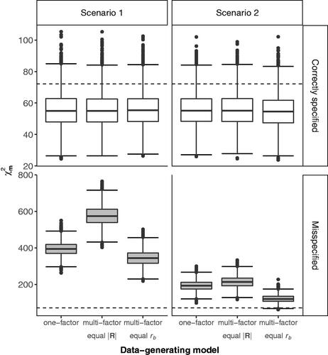
Estimating correctly-specified model results in a sample chisquare statistic ${\chi }_m^2$ of the target model m to the saturated model that has a near-zero value plus some upwards bias that is a function of sample size and the number of variables (Moshagen, 2012). The latter two data characteristics are constant across the three data-generating model conditions, which should result in similar bias magnitude. Hence, if we fit correctly-specified models to data of each of the three data-generating models, we would theoretically expect to see the exact same central chisquare distribution to pop up for the chisquare model fit statistic. Figure 1 illustrates and confirms these theoretical predictions based upon the 5000 replicates. For the chisquare statistic ${\chi }_m^2$ the distribution is indeed equivalent up to minor Monte Carlo variation under each of the three data-generating models when a correctly specified model is fitted, with about 92.5% of the 5,000 replications per data-generating model resulting in a non-statistically-significant chisquare statistic (i.e., ${\chi }_m^2\le 72.15,$ the 5% critical value for df = 54). Withstanding the difference in the amount of data correlation between the scenarios, these results do apply to both scenario 1 and scenario 2.

Figure 1. ${\chi }^2$ distribution under correctly- and misspecified models. The dotted line corresponds to the 5% critical value ${\chi }_{df=54}^2=72.15$ With ${\chi }_m^2$ chisquare of the model of interest; $\left|\mathbf{R}\right|$ determinant of the model-implied population correlation matrix as an expression of the degree of multivariate dependence; r_b within-block correlation. In both scenarios, sample size n = 200. The misspecified model is a multi-factor model for the one-factor model, and vice versa (see also Table 1).

As a corollary, given that the RMSEA is a function³ of only the target model’s chisquare, degrees of freedom, and sample size, the same equivalence of distributions across the three data generating model conditions also holds for this member of the family of parsimony fit indices. For the RMSEA, equivalent distributions were indeed observed (M = .015, and SD = .016, across all models) with values for 95% of the replicates falling in the interval $[.00,.05].$

3.1.2. Incremental Fit

The same equivalence of distribution across all of the data-generating models does not apply for the incremental fit indices, neither across scenarios nor within a scenario. For instance, although the CFI is on average as high as .99 in scenario 1, only the distribution under M1 and M2 is similar, but characterized by heavier tails in the case of M3 with a lower adjacent⁴ CFI value of .95 and a minimum of .89 compared to a lower adjacent CFI value of .97 and a minimum of .94 for both M1 and M2 (see Figure 2). When applying the commonly adopted .95 rule of thumb, this would result in assessing 4% of the correctly specified M3 models as showing non-acceptable fit to the data, compared to close to 0% for M1 and M2. With the lower amount of data correlation in scenario 2, this pattern of findings reproduces but with larger sampling variation in CFI values under all models, resulting in assessing 14 and 15% of replicates under M1 and M2 as non-acceptable according to the $\text{CFI}\ge .95$ rule of thumb with lower adjacent CFI values of .92 and .92 and minima of .81 and .84 compared to 29% of non-acceptably fitting replicates under M3 with lower adjacent CFI value of .85 and a minimum of .70.

Figure 2. CFI distribution under correctly- and misspecified models. The dotted line corresponds to the commonly adopted .95 CFI rule of thumb. With $\left|\mathbf{R}\right|$ determinant of the model-implied population correlation matrix as an expression of the degree of multivariate dependence; r_b within-block correlation. In both scenarios, sample size n = 200. The misspecified model is a multi-factor model for the one-factor model, and vice versa (see also Table 1).

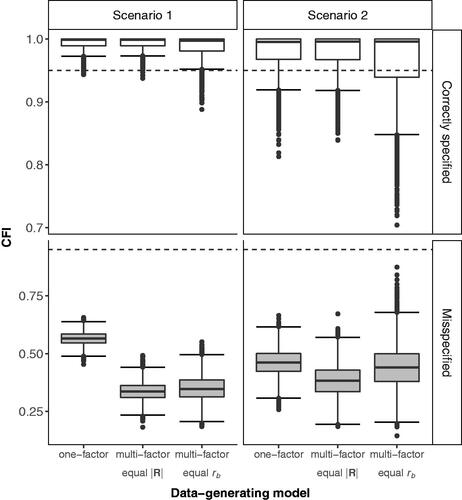
The equivalence of CFI distributions under M1 and M2 is due to both having a similar CFI numerator (i.e., based on the ${\chi }_m^2$ of a correctly specified model with the same degrees of freedom and equal sample size) and denominators with similar baseline value based on ${\chi }_0^2=-\hspace{0.17em}\text{log}\hspace{0.17em}(|\mathbf{R}|)(n-1),$ reflecting the degree of multivariate dependence in the data (see Table 1). In contrast, M3 also has a similar numerator but has a smaller baseline which makes it harder to differentiate between the model of interest and the baseline model, resulting in the heavier CFI tails under M3. In scenario 2, with the amount of data correlation being lower compared to scenario 1, the smaller baseline for all three data-generating conditions amplifies the variation in CFI including numerous observed values that are not even in line with the common rule of thumb guidelines for correctly specified models.

Trends similar to CFI’s apply to other incremental fit indices, but the increased sampling variance in scenario 2 and the heavier tail under M3 now apply to both the lower and upper tail of the distribution as both TLI and NFI are, in contrast to CFI, not restricted to an upper bound of 1. In sum, these trends show that the degree of multivariate dependence plays an integral part in the observed differences in CFI distribution, the performance of common rules of thumb, and variation in the sampling distribution of the incremental fit indices by changes in the baseline for comparison, regardless of changes in model type.

3.2. Misspecified Models

3.2.1. Absolute Fit

To consider misspecified models we fitted an orthogonal multi-factor model with independent cluster structure to data generated under M1 (one-factor model with equal loadings), and a one-factor model to data generated under models M2 and M3 (orthogonal multi-factor models with independent cluster structure and equal loadings) (see Table 1). The resulting misspecified models, denoted by M1′, M2′, and M3′, have absolute misspecification as measured by ${\chi }_{M\prime }^2$ of a similar magnitude for M1′ (${\chi }_{\mathrm{M1}\prime }^2:M=395$) and M3′ (${\chi }_{\mathrm{M3}\prime }^2:M=345$), but about one and a half times larger misspecification for M2′ (${\chi }_{\mathrm{M2}\prime }^2:M=576$) in scenario 1 (see left panel of Figure 1). For scenario 2, the chisquare values were reduced as they were bounded by the lower amount of data correlation. Differences in chisquare values between models were more compressed with M2′ still the lowest (${\chi }_{\mathrm{M2}\prime }^2:M=215$), now more closely followed by M1′ (${\chi }_{\mathrm{M1}\prime }^2:M=194$), but still a good distance to M3′ (${\chi }_{\mathrm{M3}\prime }^2:M=123$). Under each data-generating condition, the misspecified model resulted in rejecting the chisquare test of equal fit to the saturated model for almost exactly 100% of the replicates.

In terms of parsimony-adjusted absolute fit as measured by the RMSEA the chisquare values translated to an average RMSEA of .18, .22, and .16 for M1′ to M3′, respectively under scenario 1 and reduced to about half those values in scenario 2 (with the lower amounts of data correlation) to an average RMSEA of .11, .12, and .08 for M1′ to M3′, respectively. As a consequence, applying the popular rule of thumb of RMSEA below .08 in scenario 2 would wrongly assess M3′ as an acceptable fitting model for 52% of the replicates.

3.2.2. Incremental Fit

When looking at incremental fit indices, the magnitude pattern of misspecification shifts compared to the absolute fit indices. For scenario 1, M1′ results in higher incremental fit values than both M2′ and M3′, and the latter two being equal in size (e.g., see left panel of Figure 2; $\text{CFI}:M=.56,.34,$ &.35, respectively). The magnitude of CFI values seems to imply that M1′ is the least misspecified, and M2′ and M3′ the most misspecified among the three models (i.e., $\mathrm{M}1\prime <(\mathrm{M}2\prime ,\mathrm{M}3\prime )$). In contrast, the magnitude order of ${\chi }^2$ indicated M3′ and M1′ to be the least misspecified and M2′ the most misspecified (i.e., $(\mathrm{M}3\prime ,\mathrm{M}1\prime )<\mathrm{M}2\prime$).

How can these irreconcilable differences in assessment of the magnitude of model misspecification or model fit be explained? Well, M2′ and M3′ are both one-factor models wrongly fitted to data from a multi-factor, whereas M1′ is a one-factor model wrongly fitted to a multi-factor model, and hence the obvious culprit for these CFI differences must be the difference in model type? Yet, by making such an inference, we would be caught off base by not accounting for the nature of incremental fit indices and applicable baseline differences. Whereas chisquare and RMSEA are more absolute measures of misspecification (raw or parsimony-adjusted), the incremental fit indices are relative measures with the amount of absolute misspecification under the baseline model as a standardized metric.

Although M1′ and M3′ have similar ${\chi }_m^2$ values (i.e., basis of the numerator in incremental fit indices) for the target model, the baseline model in case of data generated under M1 has a larger ${\chi }_0^2$ value than under M3, leading to $\mathrm{M}1\prime >\mathrm{M}3\prime$ in CFI value. Hence, relatively speaking in CFI terms, the model M1′ is less badly misspecified compared to the baseline model for data from M1 than is the model M3′ compared to the baseline model for data from M3. Furthermore, a large ${\chi }_m^2$ is divided by a large baseline chisquare in M2′’s case and that happens to result in a CFI value similar to dividing a smaller target model chisquare by a smaller baseline chisquare in M3′’s case.

In other words, by trying to compare CFI values across models fitted on different datasets, we are looking at values on different standardized metrics as if they were comparable in an absolute sense and are now essentially ignoring the fact that we are comparing different units, literally, percentages of different baseline totals. Note that the same reasoning applies to scenario 2, although the pattern of incomparable values across models differs.

4. Implications

What all of this hopefully clarifies, is that we should resist the temptation to interpret values of incremental fit indices as if they were comparable in an absolute sense because they are only comparable in the case that their baselines are comparable at the data level (e.g., for CFI the non-centrality parameter of the baseline model λ_b) and not at the mere conceptual level (i.e., it is not sufficient that both baseline models are the null model). Such a realization has major implications for the interpretation and use of incremental fit indices, for the theoretical (im)possibility of default universal rules of thumb in their application, and for simulation studies mapping incremental fit indices as if their value is comparable in an absolute sense across any and all conditions.

4.1. Theoretical (im)Possibility of Default Universal Rules of Thumb

The fact that, in contrast to absolute fit indices, the distribution of incremental fit indices even varies across correctly specified models of equal degrees of freedom and with equal sample size (cf. compare top panels of Figures 1 and 2) implies that adopting a universally applicable general cutoff rule of thumb might not be the most fruitful idea for incremental fit indices. This is not illogical. When placing a target model of interest along a relatively small baseline-to-saturated continuum as in scenario 2 (i.e., in case of a null baseline reflected by a small value of $\left|\mathbf{R}\right|$), it will always be closely fitting in absolute sense to both the baseline and the saturated model, as all models are relatively alike. This implies that model differentiation is unreliable in case of a small baseline, incremental fit indices become less informative, and placing a fixed threshold for a universal rule of thumb becomes nigh impossible (see also, van Laar & Braeken, 2021). The opposite holds in the case of a large baseline.

4.2. Baseline Differences as Confounder in Simulation Studies

Realizing the non-ignorability of the baseline not only applies to SEM practitioners in the field, but also to past and future simulation studies where values of CFI, TLI, and family are simply tracked regardless of baseline comparability, leading to an obvious confound in their design, comparative statements, and recommendations for relative fit measures. In general, we argue that to further advance our joint understanding of goodness-of-fit measures and their behavior in practice within the SEM field, we need more theoretically driven and less exploratory simulation studies. The latter is too much at risk of making conclusions based on artifacts in the chosen design factors. One element in an exploratory study design potentially impacts many other easily overlooked confounding factors under the hood.

4.3. Determinant Not Average Pairwise Correlation

In SEM, the relative model discrepancy to the null baseline, in incremental fit indices stemming from the chisquare, does not take into account the location of the correlation in the data that your model fails to capture nor does it encode how much of the average correlation your model has captured, but instead it encodes how much of the dominant correlation (i.e., the determinant is the product of eigenvalues of R) in the data the model captures. The central role of this determinant should revive some interest in understanding classic measures of multivariate statistics (e.g., Anderson, 1958) to further our understanding of more modern SEM practices. Whereas people in practice often already find it hard to interpret the absolute magnitude of variance, it is fair to say that even fewer people have a good intuition about what a large or small determinant (i.e., generalized variance) is for their dataset.

Explicit reporting of this determinant⁵ $\left|\mathbf{R}\right|$ would help in gaining some intuition on common reference values for this data characteristic in your field of application and eventually allow for a better interpretation of the relative and absolute magnitude of incremental fit indices with the null model as a baseline, even across datasets. By making the presence of the core components of the null baseline explicit in the reporting, the need to take it into account when interpreting incremental fit indices also becomes explicit and non-ignorable (for a small reporting example and corresponding R syntax, see Appendix B).

Note that this rationale with respect to interpretation is not necessarily limited to incremental fit indices. There are other fit measures it could be extended to, even though their baseline for meaningful interpretation might be different. For example, the Standardized Root Mean Square Residual (SRMR) fit index is also a standardized measure, and hence similar interpretation and practice recommendations should apply here. The core difference to the incremental fit indices considered here is that SRMR is residual-based and not chisquare-based. As a consequence, SRMR’s metric is not a function of the determinant but of the average observed pairwise correlation $\overline{r}.$ In our small working example, the SRMR distributions for correctly specified models would indeed be equivalent under M2 and M3, but not under M1, as the former two have equal average correlation values but differ from M1’s average correlation value. In other words, SRMR evaluates fit in an average pairwise dependence sense, in contrast to incremental fit indices who evaluate fit in terms of multivariate dependence (i.e., $\left|\mathbf{R}\right|$). Realizing this difference helps in understanding what type of model fit each fit index codes for. Yet for all standardized fit indices, the base for interpretation needs to be taken into consideration and absolute value judgments across any and all conditions are not recommended.

4.4. Transferability

Although our working example is rather small, the underlying principles should apply across different scenarios. Even when extending the scope to models involving mean-structure, other baselines than the null model (e.g., Rigdon, 1998; Widaman & Thompson, 2003), non-normality corrections, or different estimation methods, the formulas for numerator and denominator and the character and metric of the baseline might slightly change, but the practical implication that incremental fit indices are only large or small in comparison to a data-specific baseline, and not a universal threshold reference value, will never disappear.

5. Practical Recommendation

CFI, TLI, and the entire incremental fit family are improperly treated in the current all too common one-off model assessment approach where they are seen as an absolute value in a mere search for a model adequacy threshold number. Instead, in a reasoned model comparison strategy, incremental fit indices are a useful benchmark metric for interpreting the relative magnitude (i.e., effect size) of the paths in which the set of competing models differ. Thus, we should strive to use incremental fit indices (Bentler & Bonett, 1980) as intended, to evaluate the relevance of cumulative theoretically motivated model restrictions in terms of % reduction in absolute misspecification as measured by the adopted baseline model.

Additional information

Funding

This study was supported by a research grant [FRIPRO-HUMSAM261769] for young research talents of the Norwegian Research Council.

Notes

1 NFI uses absolute misspecification as given by the model’s chisquare to the saturated model, CFI uses the model’s noncentrality parameter ($\lambda ={\chi }^2-\text{df}$), and TLI the ratio of chisquare to degrees of freedom of the model.

2 Given the homogeneity within and across blocks, the required within-block correlation can be obtained from the fact that the determinant for M2 reduces to the product of the within-block determinants and the relation $\left|{\mathbf{R}}_{\mathrm{M}1}\right|=[1+(I-1)r_b]{[1-r_b]}^{I-1}$(e.g., Graybill, 1983).

3 Root Mean Square Error of Approximation: $\text{RMSEA}=\frac{\sqrt{{\chi }_m^2-\text{df}}}{\sqrt{\text{df}(n-1)}}.$

4 Lower Adjacent Value: the smallest observation above or equal to the lower inner fence (i.e., first quartile minus the interquartile range) in a boxplot.

5 The determinant of the observed correlation matrix $\left|\mathbf{R}\right|$ can be easily extracted from default software. For R::lavaan, this can be extracted from the fitted model, in the example syntax stored in an object labeled “fit”: exp(−(fitmeasures(fit)[["baseline.chisq"]]/(inspect(fit, "nobs")−1))).

Appendix A.

The Chisquare of the Null Model is Proportional to Minus the log Determinant of the Observed Correlation Matrix (${\chi }_0^2\propto -\hspace{0.17em}\text{log}\hspace{0.17em}\left|\mathbf{R}\right|$)

For the default CFI with a null model as baseline, the value of CFI is based on the ratio of misspecification between the model of interest and the null model: (1) $${\text{CFI}}_{(m,0)}=1-\frac{{\lambda }_m}{{\lambda }_0}=1-\frac{{\chi }_m^2-{\text{df}}_m}{{\chi }_0^2-{\text{df}}_0}$$(1)

Equation (1)(1) $${\text{CFI}}_{(m,0)}=1-\frac{{\lambda }_m}{{\lambda }_0}=1-\frac{{\chi }_m^2-{\text{df}}_m}{{\chi }_0^2-{\text{df}}_0}$$(1) shows how the misspecification of both models would be estimated by their non-centrality parameter, being the difference between the model’s chisquare of exact fit against the saturated model and the model’s degrees of freedom. Focusing on the denominator of CFI, the standard of comparison, and hence the core component of CFI, is then ${\chi }_0^2-\mathrm{d}{\mathrm{f}}_0,$ the chisquare of the null model with degrees of freedom $\mathrm{d}{\mathrm{f}}_0=I(I-1)/2)$ and I the number of manifest variables. The chisquare value of the null model can be rewritten as the product of the sample size n and the minimum value F₀ of the used fit function to estimate the models (i.e., ${\chi }_0^2=F_0(n-1)$).

Under maximum likelihood estimation, F₀ is a function of the discrepancy between the model-implied variance-covariance matrix ${\widehat{\mathbf{\Sigma }}}_0$ under the null model and the observed variance-covariance matrix S (e.g., Bollen, 1989), where $\text{tr}(\mathbf{X})$ and $\left|\mathbf{X}\right|$ are respectively the trace and determinant of a matrix X (cf. Equation (2)(2) $$F_0=\hspace{0.17em}\text{log}\hspace{0.17em}\left|{\widehat{\mathbf{\Sigma }}}_0\right|-\hspace{0.17em}\text{log}\hspace{0.17em}\left|\mathbf{S}\right|+\text{tr}(\mathbf{S}{\widehat{\mathbf{\Sigma }}}_0^{-1})-I$$(2) ). (2) $$F_0=\hspace{0.17em}\text{log}\hspace{0.17em}\left|{\widehat{\mathbf{\Sigma }}}_0\right|-\hspace{0.17em}\text{log}\hspace{0.17em}\left|\mathbf{S}\right|+\text{tr}(\mathbf{S}{\widehat{\mathbf{\Sigma }}}_0^{-1})-I$$(2) (3) $$=\hspace{0.17em}\text{log}\hspace{0.17em}|\mathbf{diag}(\mathbf{S})|-\hspace{0.17em}\text{log}\hspace{0.17em}\left|\mathbf{S}\right|+\text{tr}(\mathbf{Sdiag}{(\mathbf{S})}^{-1})-I$$(3) (4) $$=\hspace{0.17em}\text{log}\hspace{0.17em}|\mathbf{diag}(\mathbf{S})|-\hspace{0.17em}\text{log}\hspace{0.17em}\left|\mathbf{S}\right|+I-I$$(4)

Key in getting to the expression for the chisquare ${\chi }_0^2$ for the null model as mentioned in the main text (i.e., $-\hspace{0.17em}\text{log}\hspace{0.17em}\left|\mathbf{R}\right|$ up to a sample size factor), is that the minimal fit value F₀ for the null model can be further simplified using the fact that the model-implied covariance matrix under the null model comes down to a diagonal matrix $\mathbf{diag}(\mathbf{S})$ with the observed variances on the diagonal (cf. Equation (3)(3) $$=\hspace{0.17em}\text{log}\hspace{0.17em}|\mathbf{diag}(\mathbf{S})|-\hspace{0.17em}\text{log}\hspace{0.17em}\left|\mathbf{S}\right|+\text{tr}(\mathbf{Sdiag}{(\mathbf{S})}^{-1})-I$$(3) ). This results in $\mathbf{S}{\widehat{\mathbf{\Sigma }}}_0^{-1}$ leading to a matrix with all ones on the diagonal such that the trace equals the number of observed variables I and cancels out the subsequent – I term in the expression for F₀ (cf. Equation (4)(4) $$=\hspace{0.17em}\text{log}\hspace{0.17em}|\mathbf{diag}(\mathbf{S})|-\hspace{0.17em}\text{log}\hspace{0.17em}\left|\mathbf{S}\right|+I-I$$(4) ).

Using the fact that the determinant of a matrix product can be split into products of determinants, each of the remaining two log determinants can be written out given that a variance-covariance matrix S is a multiplicative function of a corresponding correlation matrix R and an inverse diagonal matrix with standard deviations on the diagonal. Thus we have (5) $$\text{log}\hspace{0.17em}\left|\mathbf{S}\right| =\hspace{0.17em}\text{log}\hspace{0.17em}\left|\sqrt{\mathbf{diag}(\mathbf{S})}\mathbf{R}\sqrt{\mathbf{diag}(\mathbf{S})}\right|$$(5) (6) $$=\hspace{0.17em}\text{log}\hspace{0.17em}\left|\sqrt{\mathbf{diag}(\mathbf{S})}\right|+\hspace{0.17em}\text{log}\hspace{0.17em}\left|\mathbf{R}\right|+\hspace{0.17em}\text{log}\hspace{0.17em}\left|\sqrt{\mathbf{diag}(\mathbf{S})}\right|$$(6) (7) $$=\hspace{0.17em}\text{log}\hspace{0.17em}\prod _{j=1}^I\sqrt{S_{jj}}+\hspace{0.17em}\text{log}\hspace{0.17em}\left|\mathbf{R}\right|+\hspace{0.17em}\text{log}\hspace{0.17em}\prod _{j=1}^I\sqrt{S_{jj}}$$(7) (8) $$=\hspace{0.17em}\text{log}\hspace{0.17em}\prod _{j=1}^I{S}_{jj}+\hspace{0.17em}\text{log}\hspace{0.17em}\left|\mathbf{R}\right|$$(8) and (9) $$\text{log}\hspace{0.17em}|\mathbf{diag}(\mathbf{S})|=\hspace{0.17em}\text{log}\hspace{0.17em}\left|\sqrt{\mathbf{diag}(\mathbf{S})}\mathbf{I}\sqrt{\mathbf{diag}(\mathbf{S})}\right|$$(9) (10) $$=\hspace{0.17em}\text{log}\hspace{0.17em}\prod _{j=1}^I{S}_{jj}+0$$(10) where Equation (10)(10) $$=\hspace{0.17em}\text{log}\hspace{0.17em}\prod _{j=1}^I{S}_{jj}+0$$(10) makes use of the fact that the correlation matrix of a diagonal variance-covariance matrix is an identity matrix I which determinant is exactly equal to 1.

The re-expressions of the log determinant terms in Equations (8)(8) $$=\hspace{0.17em}\text{log}\hspace{0.17em}\prod _{j=1}^I{S}_{jj}+\hspace{0.17em}\text{log}\hspace{0.17em}\left|\mathbf{R}\right|$$(8) and (10)(10) $$=\hspace{0.17em}\text{log}\hspace{0.17em}\prod _{j=1}^I{S}_{jj}+0$$(10) allow to simplify the expression for F₀ further by elimination (11) $$F_0=\hspace{0.17em}\text{log}\hspace{0.17em}|\mathbf{diag}(\mathbf{S})|-\hspace{0.17em}\text{log}\hspace{0.17em}\left|\mathbf{S}\right|$$(11) (12) $$=\hspace{0.17em}\text{log}\hspace{0.17em}\prod _{j=1}^I{S}_{jj}-\hspace{0.17em}\text{log}\hspace{0.17em}\prod _{j=1}^I{S}_{jj}-\hspace{0.17em}\text{log}\hspace{0.17em}\left|\mathbf{R}\right|$$(12) (13) $$=-\hspace{0.17em}\text{log}\hspace{0.17em}\left|\mathbf{R}\right|$$(13) such that the denominator of CFI under the null model comes down to $${\lambda }_0={\chi }_0^2-{\text{df}}_0=F_0(n-1)-{\text{df}}_0=-\hspace{0.17em}\text{log}\hspace{0.17em}\left|\mathbf{R}\right|(n-1)-I(I-1)/2$$

Appendix B.

Mini Example to Report Incremental Fit Indices with Corresponding R::Lavaan Code

The SEM-package lavaan (Rosseel, 2012) in the free statistical software environment R (R Core Team, 2020) contains a built-in dataset variant of a well-known study by Holzinger and Swineford (1939). Situated in the study of human intelligence, the dataset contains scores on I = 9 cognitive ability tests (named variables x1 to x9 in the dataset) for n = 301 children. In practice, we advocate the use of incremental fit indices as intended, that is in the context of a reasoned model comparison strategy. Without being able to elaborate too much on specifics of the field or dataset, we can still posit a fairly realistic set of competing models for the current context as an example in case, but with a somewhat simplified underlying theoretical motivation.

Set of Competing Models

A historical finding in the intelligence field is that cognitive tests, no matter their specifics, tend to positively correlate within a general population. This would correspond to a so-called positive manifold as reflected by the appropriateness of a one-factor model ${\mathrm{M}}_1$ covering all 9 tests. Yet the nine cognitive tests are said to have some common structural elements, with the first three tests being more the visuo-spatial type, the second three tests being more verbal-text related, and the last three more speed-based. It would be natural to expect these clusters to also be reflected in the strength of the intercorrelations between the test scores. Yet how this exactly surfaces, one can disagree about. Model ${\mathrm{M}}_{2a}$ considers three orthogonal factors, one for each of the three independent item clusters. This model also implies that intercorrelations among cognitive tests of a different type would be negligible. Model ${\mathrm{M}}_{2b}$ with three oblique factors, one for each of the three independent item clusters, offers a less strict perspective by implying that the dominant correlation is within the clusters but allowing some correlation between clusters. A final model ${\mathrm{M}}_3$ covers all bases by considering a one-factor model but with residual correlations among cognitive tests within the same cluster.

The model comparison strategy further involves locating the set of competing models within a continuum of models from the worst fitting baseline null model ${\mathrm{M}}_0$ to the perfect fitting saturated model ${\mathrm{M}}_S$ (Bentler & Bonett, 1980). The results are summarized and reported in Table B.1. Corresponding R-code for the models and results can be found at https://osf.io/f6jnm/?view_only=e367c654fbcd47248667e170442592c3.

Table B.1. Model comparison results for the set of competing models.

	${\mathrm{M}}_0$	${\mathrm{M}}_1$	${\mathrm{M}}_{2a}$	${\mathrm{M}}_{2b}$	${\mathrm{M}}_3$	${\mathrm{M}}_S$
${\chi }^2$	919	312	154	85	35	0
df	36	27	27	24	18	0
p	<.001	<.001	<.001	<.001	0.010	1.000
λ	883	285	127	61	17	0
${\text{CFI}}_{(m,0)}$	0.00	0.68	0.86	0.93	0.98	1.00
$\left|\mathbf{R}\right|=0.047$, n = 301, I = 9.

Note. λ = non-centrality for the estimated model (i.e., $\lambda ={\chi }^2-\text{df}$); CFI = CFI value for estimated model (i.e., ${\text{CFI}}_{(m,0)}=1-\frac{{\lambda }_m}{{\lambda }_0}$); $\left|\mathbf{R}\right|$ = determinant of the observed correlation matrix (i.e., the degree of multivariate dependence); n = sample size; I = number of items. Here one would typically further clarify the model specifications and highlight the differences among the models. Yet, to keep the appendix compact see the text above.

Results

We can see that accounting for the implied positive manifold or the expectation that performance on cognitive tests correlates by default as in ${\mathrm{M}}_1,$ reduces the specification error in terms of the multivariate degree of dependence present in the data by 68% (${\text{CFI}}_{({\mathrm{M}}_1,{\mathrm{M}}_0)}=.68$). Note how in linear regression, one would generally already be quite happy with such a relative reduction in predictor error variance as implied by an r-square of .68. Although the model does not fit close to perfect in an absolute sense, there is sufficient to disregard the implied uncorrelatedness of test performances by model ${\mathrm{M}}_0.$ At the same time, we see that ignoring the positive manifold idea and only accounting for the cluster structure as in ${\mathrm{M}}_{2a}$ leads to a reduction of 86%, an additional 18% reduction in misspecification error of the multivariate dependence compared to ${\mathrm{M}}_1.$ This finding implies that the dominant correlation structure in the dataset is indeed between cognitive tests of the same type. Allowing for some structural intercorrelation between the clusters does reduce misspecification somewhat more with an additional 7%, amount to a total reduction of 93% under ${\mathrm{M}}_{2b}.$ Further covering both perspectives with a structural positive manifold and variable residual interdependence within a cluster, as in ${\mathrm{M}}_3,$ leads to an additional reduction of 5% in misspecification error, bringing us, relatively speaking within 2% (${\text{CFI}}_{({\mathrm{M}}_3,{\mathrm{M}}_0)}$ =.98), in the immediate neighborhood of the ‘perfect’ yet unstructured saturated model ${\mathrm{M}}_S.$

Simplified Conclusion

In a reasoned model comparison strategy, incremental fit indices are a useful benchmark metric for interpreting the relative magnitude (i.e., effect size) of the paths in which the set of competing models differ. Together these results imply that the paths corresponding to the cluster structure in terms of cognitive test type are clearly pronounced, but that not all cognitive tests adhere to a strict clustering and still intercorrelate across types as well. When inspecting the correlation matrix among the cognitive tests, you can also clearly see the cluster structure, but also the first visuo-spatial test correlating with the majority of other tests regardless of type.

Notice that in our assessments there was no explicit need for rules of thumb nor a focus on absolute fit, as in the end interest would be more about strengths of the different perspectives as put forward by the competing models. This appears to us as a more healthy approach than a one-off model assessment approach using binary conclusions based on indefensible universal rules of thumb (e.g. CFI≥.95). For one specific study, the value of reporting determinant, sample size, and number of variables might not be directly apparent. Yet, these summary statistics would become relevant once you intend to compare incremental fit indices across different studies to assess whether one study’s 93% is comparable to another study’s 95%, and for general meta-analysis purposes. Hence, we recommend including these by default, and doing so is luckily extremely simple in practice.

References

- Anderson, T. (1958). An introduction to multivariate statistical analysis. Wiley.
- Baguley, T. (2009). Standardized or simple effect size: What should be reported? British Journal of Psychology, 100, 603–617.
- Beauducel, A., & Wittmann, W. W. (2005). Simulation study on fit indexes in CFA based on data with slightly distorted simple structure. Structural Equation Modeling: A Multidisciplinary Journal, 12, 41–75.
- Bentler, P. M. (1990). Comparative fit indexes in structural models. Psychological Bulletin, 107, 238–246.
- Bentler, P. M., & Bonett, D. G. (1980). Significance tests and goodness of fit in the analysis of covariance structures. Psychological Bulletin, 88, 588–606.
- Bollen, K. A. (1989). Structural equations with latent variables. John Wiley & Sons, Inc.
- Fan, X., & Sivo, S. A. (2007). Sensitivity of fit indices to model misspecification and model types. Multivariate Behavioral Research, 42, 509–529.
- Graybill, F. A. (1983). Matrices with applications in statistics (2nd ed.). Wadsworth International Group.
- Holzinger, K. J., & Swineford, F. (1939). A study in factor analysis: The stability of a bi-factor solution. University of Chicago Press.
- Hu, L., & Bentler, P. M. (1999). Cutoff criteria for fit indexes in covariance structure analysis: Conventional criteria versus new alternatives. Structural Equation Modeling: A Multidisciplinary Journal, 6, 1–55.
- Jackson, D. L., Gillaspy, J. A., & Purc-Stephenson, R. (2009). Reporting practices in confirmatory factor analysis: An overview and some recommendations. Psychological Methods, 14, 6–23.
- Lai, K., & Green, S. B. (2016). The problem with having two watches: Assessment of fit when RMSEA and CFI disagree. Multivariate Behavioral Research, 51, 220–239.
- Marsh, H. W., Balla, J. R., & McDonald, R. P. (1988). Goodness-of-fit indexes in confirmatory factor analysis: The effect of sample size. Psychological Bulletin, 103, 391–410.
- McDonald, R. P., & Ho, M. R. (2002). Principles and practice in reporting structural equation analyses. Psychological Methods, 7, 64–82.
- Moshagen, M. (2012). The model size effect in SEM: Inflated goodness-of-fit statistics are due to the size of the covariance matrix. Structural Equation Modeling: A Multidisciplinary Journal, 19, 86–98.
- Niemand, T., & Mai, R. (2018). Flexible cutoff values for fit indices in the evaluation of structural equation models. Journal of the Academy of Marketing Science, 46, 1148–1172.
- R Core Team (2020). R: A language and environment for statistical computing.
- Raykov, T. (2005). Bias-corrected estimation of noncentrality parameters of covariance structure models. Structural Equation Modeling: A Multidisciplinary Journal, 12, 120–129.
- Rigdon, E. E. (1998). The equal correlation baseline model for comparative fit assessment in structural equation modeling. Structural Equation Modeling: A Multidisciplinary Journal, 5, 63–77.
- Rosseel, Y. (2012). lavaan: An R package for structural equation modeling. Journal of Statistical Software, 48, 1–36.
- Tucker, L. R., & Lewis, C. (1973). A reliability coefficient for maximum likelihood factor analysis. Psychometrika, 38, 1–10.
- van Laar, S., & Braeken, J. (2021). Understanding the comparative fit index: It’s all about the base! Practical Assessment, Research, and Evaluation, 26, Article 26. https://doi.org/10.7275/23663996
- Widaman, K. F., & Thompson, J. S. (2003). On specifying the null model for incremental fit indices in structural equation modeling. Psychological Methods, 8, 16–37.
- Yuan, K.-H., & Bentler, P. M. (2000). Three likelihood-based methods for mean and covariance structure analysis with nonnormal missing data. Sociological Methodology, 30, 165–200.