A Faster Procedure for Estimating SEMs Applying Minimum Distance Estimators With a Fixed Weight Matrix

Abstract

This study presents a separable nonlinear least squares (SNLLS) implementation of the minimum distance (MD) estimator employing a fixed-weight matrix for estimating structural equation models (SEMs). In contrast to the standard implementation of the MD estimator, in which the complete set of parameters is estimated using nonlinear optimization, the SNLLS implementation allows a subset of parameters to be estimated using (linear) least squares (LS). The SNLLS implementation possesses a number of benefits, such as faster convergence, better performance in ill-conditioned estimation problems, and fewer required starting values. The present work demonstrates that SNLLS, when applied to SEM estimation problems, significantly reduces the estimation time. Reduced estimation time makes SNLLS particularly useful in applications involving some form of resampling, such as simulation and bootstrapping.

Keywords:

• Minimum distance estimation
• numerical efficiency
• quadratic form fit function
• structural equation models

1. Introduction

This study addresses the application of separable nonlinear least squares (SNLLS) when performing covariance structure analysis (CSA). SNLLS was first introduced by Golub and Pereyra (1973), who showed that for a certain type of nonlinear estimation problems, a subset of parameters can be estimated using numerically efficient least squares (LS). As will be discussed below, several studies have shown that parameter separation offers a number of numerical benefits, such as faster convergence, better performance when the estimation problem is ill-conditioned (i.e., problems in which the ratio between the largest and the smallest singular value of the covariance matrix is large), and fewer required starting values.

SNLLS is typically applied to problems involving some form of nonlinear regression analysis, but not exclusively so. A recent study by Kreiberg et al. (2021) suggested an SNLLS implementation of the minimum distance (MD) estimator for estimating confirmatory factor analysis (CFA) models. The motivation for the current study is to generalize the results in Kreiberg et al. (2021) by outlining an SNLLS implementation for estimating structural equation models (SEMs). This is important for several reasons. First, it makes SNLLS applicable to a wider range of models. Second, at this stage, little is known about the potential benefits of applying SNLLS in the context of CSA. The outlined SNLLS implementation may pave the way for future research on how to improve the numerical performance of CSA based estimators.

To make the idea of SNLLS clearer, consider the familiar MD quadratic form objective function (1) $$F\left(\mathit{\vartheta }\right)={\left({\mathit{s}}_x-{\mathit{\sigma }}_x\left(\mathit{\vartheta }\right)\right)}^T\mathit{V}\left({\mathit{s}}_x-{\mathit{\sigma }}_x\left(\mathit{\vartheta }\right)\right),$$(1) where ${\mathit{s}}_x$ and ${\mathit{\sigma }}_x\left(\mathit{\vartheta }\right)$ are covariance vectors derived from the sample and the model, respectively, $\mathit{\vartheta }$ is the parameter vector and $\mathit{V}$ is a weighting matrix chosen by the user. We consider the case in which $\mathit{V}$ is a fixed matrix (i.e., when $\mathit{V}$ is not a function of $\mathit{\vartheta }$). Such cases include well-known estimators such as unweighted least squares (ULS), generalized least squares (GLS), and weighted least squares (WLS). The standard implementation of Equation (1)(1) $$F\left(\mathit{\vartheta }\right)={\left({\mathit{s}}_x-{\mathit{\sigma }}_x\left(\mathit{\vartheta }\right)\right)}^T\mathit{V}\left({\mathit{s}}_x-{\mathit{\sigma }}_x\left(\mathit{\vartheta }\right)\right),$$(1) is a one-step estimation procedure, here referred to as nonlinear least squares (NLLS), that involves the use of nonlinear optimization techniques. Estimation is performed by searching the parameter space for the value of $\mathit{\vartheta }$ that minimizes Equation (1)(1) $$F\left(\mathit{\vartheta }\right)={\left({\mathit{s}}_x-{\mathit{\sigma }}_x\left(\mathit{\vartheta }\right)\right)}^T\mathit{V}\left({\mathit{s}}_x-{\mathit{\sigma }}_x\left(\mathit{\vartheta }\right)\right),$$(1) . In contrast, the SNLLS implementation of Equation (1)(1) $$F\left(\mathit{\vartheta }\right)={\left({\mathit{s}}_x-{\mathit{\sigma }}_x\left(\mathit{\vartheta }\right)\right)}^T\mathit{V}\left({\mathit{s}}_x-{\mathit{\sigma }}_x\left(\mathit{\vartheta }\right)\right),$$(1) is a two-step estimation procedure that works by splitting $\mathit{\vartheta }$ into two subsets. In the first step, one subset of parameters is estimated using nonlinear optimization. In the second step, based on the estimates obtained in the first step, the remaining subset of parameters is estimated using LS. As demonstrated in Kreiberg et al. (2021), SNLLS provides parameter estimates and a minimum objective function value identical to those obtained using NLLS. It obviously follows that the asymptotic properties of the estimator are maintained. The presentation below presents a general framework for how to accomplish parameter separation in the case of SEMs.

Over the years, SNLLS has become popular in applied research across a wide range of scientific disciplines. Golub and Pereyra (2003) compiled a list of real-world examples of SNLLS applications. Mullen (2008) subsequently provided a comprehensive overview of SNLLS for a number of applications in physics and chemistry. SNLLS has also proved useful in systems and control applications. For instance, Söderström et al. (2009), Söderström & Mossberg (2011), and Kreiberg et al. (2016) applied CSA to handle the errors-in-variables (EIV) estimation problem. The work in these studies showed how to implement the MD estimator using SNLLS.

Several studies have documented that the SNLLS implementation of nonlinear estimators offers a number of benefits. For instance, Sjöberg and Viberg (1997) evaluated the numerical performance of SNLLS when applied to neural-network minimization problems. Their main conclusions were that SNLLS provides faster convergence and performs better in cases in which the estimation problem is ill-conditioned. A recent study by Dattner et al. (2020) investigated the performance of SNLLS when applied to estimation problems involving ordinary differential equations (ODEs). Their simulations showed that SNLLS provides faster convergence as well as parameter estimates of similar or higher accuracy than what is achieved by traditional nonlinear procedures.

The remainder of this article is organized as follows. Section 2 establishes the notation used throughout the article. In this section, we provide a brief overview of the SEM framework and the associated MD estimator. Section 3 outlines how to modify the MD objective function to accommodate the SNLLS implementation of the estimator when applied to SEMs. Section 4 compares the numerical efficiency of SNLLS and NLLS when applied to real-world estimation problems. Finally, Section 5 presents some concluding remarks.

2. Background

2.1. Notation

Before presenting the SEM framework, it will be useful to introduce the following notation. Let $\mathit{x}$ be a $p\times 1$ zero-mean random vector, and let ${\mathit{\Sigma }}_x$ be the associated $p\times p$ covariance matrix given by (2) $${\mathit{\Sigma }}_x=E\left[\mathit{x}{\mathit{x}}_{\mathrm{\hspace{0.17em}}}^T\right],$$(2) where $E$ is the expectation operator and the superscript T is the transpose of a vector or a matrix. The number of nonredundant elements in ${\mathit{\Sigma }}_x$ is $h=2^{-1}p\left(p+1\right),$ given that no restrictions other than symmetry are placed on the elements of ${\mathit{\Sigma }}_x.$ A covariance vector containing the nonredundant elements (i.e., the lower half of ${\mathit{\Sigma }}_x$ including the diagonal) is (3) $${\mathit{\sigma }}_x=\mathit{vech}\left({\mathit{\Sigma }}_x\right).$$(3) In this expression, $\mathit{vech}$ is the operation of vectorizing the nonredundant elements of ${\mathit{\Sigma }}_x.$ Alternatively, ${\mathit{\sigma }}_x$ is obtained by (4) $${\mathit{\sigma }}_x={\mathit{K}}_x^{T}vec\left({\mathit{\Sigma }}_x\right).$$(4) Here, $\mathit{vec}$ is the operation of vectorizing the elements of a matrix by stacking its columns, and ${\mathit{K}}_x$ is a $p^2\times h$ matrix obtained from (5) $${\mathit{K}}_x={\mathit{L}}_x{\left({\mathit{L}}_x^T{\mathit{L}}_x\right)}^{-1},$$(5) where ${\mathit{L}}_x$ is a $p^2\times h$ selection matrix containing only ones and zeros. This matrix has the additional usage (6) $$\mathit{vec}\left({\mathit{\Sigma }}_x\right)={\mathit{L}}_x{\mathit{\sigma }}_x.$$(6) In the case of symmetry, ${\mathit{L}}_x$ is referred to as the duplication matrix in the literature (see Magnus & Neudecker, 1999). The matrices ${\mathit{L}}_x$ and ${\mathit{K}}_x$ can be formed to handle covariance matrices with additional structure beyond symmetry. For instance, in the case that ${\mathit{\Sigma }}_x$ is a diagonal, ${\mathit{K}}_x$ is constructed so that ${\mathit{\sigma }}_x$ contains only the elements on the diagonal of ${\mathit{\Sigma }}_x.$ Appendix A outlines a general framework for how to obtain ${\mathit{L}}_x$ and ${\mathit{K}}_x$ for various structures characterizing ${\mathit{\Sigma }}_x.$

We now expand the previous notation. Let ${\mathit{x}}_1$ and ${\mathit{x}}_2$ be $p_1\times 1$ and $p_2\times 1$ zero-mean random vectors, respectively. A $p=p_1+p_2$ dimensional column vector is given by (7) $$\mathit{x}={\left({\mathit{x}}_1^T\mathrm{ }{\mathit{x}}_2^T\right)}^T.$$(7) The associated $p\times p$ covariance matrix is (8) $${\mathit{\Sigma }}_x=\left(\begin{array}{cc}\underset{\left(p_1\times p_1\right)}{{\mathit{\Sigma }}_{x_1}}& \underset{\left(p_1\times p_2\right)}{{\mathit{\Sigma }}_{x_2,x_1}^T}\\ \underset{\left(p_2\times p_1\right)}{{\mathit{\Sigma }}_{x_2,x_1}}& \underset{\left(p_2\times p_2\right)}{{\mathit{\Sigma }}_{x_2}}\end{array}\right),$$(8) where (9) $${\mathit{\Sigma }}_{x_1}=E\left[{\mathit{x}}_1{\mathit{x}}_1^T\right],\mathrm{ }{\mathit{\Sigma }}_{x_2}=E\left[{\mathit{x}}_2{\mathit{x}}_2^T\right],\mathrm{ }{\mathit{\Sigma }}_{x_2,x_1}=E\left[{\mathit{x}}_2{\mathit{x}}_1^T\right].$$(9)

As before, the vector consisting of the nonredundant elements of ${\mathit{\Sigma }}_x$ is given by ${\mathit{\sigma }}_x.$ However, for later, it will be more convenient to work with the vector (10) $${\stackrel{\sim }{\mathit{\sigma }}}_x={\left({\mathit{\sigma }}_{x_1}^T\mathrm{ }{\mathit{\sigma }}_{x_2}^T\mathrm{ }{\mathit{\sigma }}_{x_2,x_1}^T\right)}^T,$$(10) where (11) $${\mathit{\sigma }}_{x_1}={\mathit{K}}_{x_1}^{T}vec\left({\mathit{\Sigma }}_{x_1}\right), {\mathit{\sigma }}_{x_2}={\mathit{K}}_{x_2}^{T}vec\left({\mathit{\Sigma }}_{x_2}\right), {\mathit{\sigma }}_{x_2,x_1}=\mathit{vec}\left({\mathit{\Sigma }}_{x_2,x_1}\right).$$(11)

Note that ${\stackrel{\sim }{\mathit{\sigma }}}_{\mathit{x}}$ contains the same elements as ${\mathit{\sigma }}_x,$ but in a different order. The last equation in Equation (11)(11) $${\mathit{\sigma }}_{x_1}={\mathit{K}}_{x_1}^{T}vec\left({\mathit{\Sigma }}_{x_1}\right), {\mathit{\sigma }}_{x_2}={\mathit{K}}_{x_2}^{T}vec\left({\mathit{\Sigma }}_{x_2}\right), {\mathit{\sigma }}_{x_2,x_1}=\mathit{vec}\left({\mathit{\Sigma }}_{x_2,x_1}\right).$$(11) follows from the fact that there is no redundancy in ${\mathit{\Sigma }}_{x_2,x_1}.$ Appendix A shows how to derive a matrix ${\stackrel{\sim }{\mathit{L}}}_x.$ Then, by using Equations (4)(4) $${\mathit{\sigma }}_x={\mathit{K}}_x^{T}vec\left({\mathit{\Sigma }}_x\right).$$(4) and (5)(5) $${\mathit{K}}_x={\mathit{L}}_x{\left({\mathit{L}}_x^T{\mathit{L}}_x\right)}^{-1},$$(5) , we obtain the covariance vector (12) $${\stackrel{\sim }{\mathit{\sigma }}}_x={\stackrel{\sim }{\mathit{K}}}_x^{T}vec\left({\mathit{\Sigma }}_x\right).$$(12)

2.2. The SEM Framework

With the basic notation in place, we are ready to introduce the SEM framework, which consists of the following three equations (excluding constant terms) (13) $$\mathit{\eta }=\mathit{B}\mathit{\eta }+\mathit{\Gamma }\mathit{\xi }+\mathit{\delta },$$(13) (14) $${\mathit{x}}_1={\mathit{\Lambda }}_1\mathit{\eta }+{\mathit{ϵ}}_1,$$(14) (15) $${\mathit{x}}_2={\mathit{\Lambda }}_2\mathit{\xi }+{\mathit{ϵ}}_2.$$(15) The first equation is the structural equation, which specifies the causal relationships among the latent variables. In this equation, $\mathit{\eta }$ and $\mathit{\xi }$ are respectively $p_{\mathit{\eta }}\times 1$ and $p_{\xi }\times 1$ random vectors, $\mathit{\delta }$ is a $p_{\eta }\times 1$ random noise vector, and $\mathit{B}$ and $\mathit{\Gamma }$ are respectively $p_{\eta }\times p_{\eta }$ and $p_{\eta }\times p_{\xi }$ parameter matrices relating the latent random vectors. The last two equations are measurement equations. In these equations, ${\mathit{x}}_1$ and ${\mathit{x}}_2$ are respectively $p_1\times 1$ and $p_2\times 1$ observed random vectors, ${\mathit{ϵ}}_1$ and ${\mathit{ϵ}}_2$ are noise vectors of similar dimensions, and ${\mathit{\Lambda }}_1$ and ${\mathit{\Lambda }}_2$ are respectively $p_1\times p_{\eta }$ and $p_2\times p_{\xi }$ parameter matrices relating the observed and the latent random vectors. All random vectors are zero-mean.

It is assumed that $\mathit{I}-\mathit{B}$, where I is the identity matrix, is nonsingular such that $\mathit{\eta }$ is uniquely determined by $\mathit{\xi }$ and $\mathit{\delta }.$ It is further assumed that $\mathit{\delta }$ and $\mathit{\xi }$ are mutually uncorrelated, and that ${\mathit{ϵ}}_1$ and ${\mathit{ϵ}}_2$ are mutually uncorrelated with $\mathit{\eta }$ and $\mathit{\xi },$ respectively. The noise vectors ${\mathit{ϵ}}_1$ and ${\mathit{ϵ}}_2$ are allowed to correlate.

The specification additionally includes the following covariance matrices (16) $$\begin{array}{l}{\mathit{\Sigma }}_{\xi }=E\left[\mathit{\xi }{\mathit{\xi }}^T\right],\mathrm{ }{\mathit{\Sigma }}_{\delta }=E\left[\mathit{\delta }{\mathit{\delta }}_{\mathrm{\hspace{0.17em}}}^T\right],\mathrm{ }{\mathit{\Sigma }}_{{ϵ}_1}=E\left[{\mathit{ϵ}}_1{\mathit{ϵ}}_1^T\right],\\ {\mathit{\Sigma }}_{{ϵ}_2}=E\left[{\mathit{ϵ}}_2{\mathit{ϵ}}_2^T\right],\mathrm{ }{\mathit{\Sigma }}_{{ϵ}_2,{ϵ}_1}=E\left[{\mathit{ϵ}}_2{\mathit{ϵ}}_1^T\right].\end{array}\mathrm{ }$$(16) The nonredundant elements of ${\mathit{\Sigma }}_{\xi },$ ${\mathit{\Sigma }}_{\delta },$ ${\mathit{\Sigma }}_{{ϵ}_1},$ ${\mathit{\Sigma }}_{{ϵ}_2}$ and ${\mathit{\Sigma }}_{{ϵ}_2,{ϵ}_1}$ are given by the covariance vectors (17) $$\begin{array}{l}{\mathit{\sigma }}_{\xi }={\mathit{K}}_{\xi }^{T}vec\left({\mathit{\Sigma }}_{\xi }\right),\mathrm{ }{\mathit{\sigma }}_{\delta }={\mathit{K}}_{\delta }^{T}vec\left({\mathit{\Sigma }}_{\delta }\right),\mathrm{ }{\mathit{\sigma }}_{{ϵ}_1}={\mathit{K}}_{{ϵ}_1}^{T}vec\left({\mathit{\Sigma }}_{{ϵ}_1}\right),\\ {\mathit{\sigma }}_{{ϵ}_2}={\mathit{K}}_{{ϵ}_2}^{T}vec\left({\mathit{\Sigma }}_{{ϵ}_2}\right),\mathrm{ }{\mathit{\sigma }}_{{ϵ}_2,{ϵ}_1}=\mathit{vec}\left({\mathit{\Sigma }}_{{ϵ}_2,{ϵ}_1}\right).\end{array}$$(17) Let $\mathit{\vartheta }$ be a parameter vector containing the free elements in $\mathit{B},$ $\mathit{\Gamma },$ ${\mathit{\Lambda }}_1,$ ${\mathit{\Lambda }}_2,$ ${\mathit{\Sigma }}_{\xi },$ ${\mathit{\Sigma }}_{\delta },$ ${\mathit{\Sigma }}_{{ϵ}_1},$ ${\mathit{\Sigma }}_{{ϵ}_2}$ and ${\mathit{\Sigma }}_{{ϵ}_2,{ϵ}_1},$ and let $\mathit{H}={\left(\mathit{I}-\mathit{B}\right)}^{-1}.$ The covariance matrix implied by Equations (13)–(15) is (18) $${\mathit{\Sigma }}_x\left(\mathit{\vartheta }\right)=\left(\begin{array}{ll}{\mathit{\Lambda }}_1\mathit{H}\left(\mathit{\Gamma }{\mathit{\Sigma }}_{\xi }{\mathit{\Gamma }}^T+{\mathit{\Sigma }}_{\delta }\right){\mathit{H}}^T{\mathit{\Lambda }}_1^T+{\mathit{\Sigma }}_{{ϵ}_1}& {\mathit{\Lambda }}_1\mathit{H}\mathit{\Gamma }{\mathit{\Sigma }}_{\xi }{\mathit{\Lambda }}_2^T+{\mathit{\Sigma }}_{{ϵ}_2,{ϵ}_1}^T\\ {\mathit{\Lambda }}_2{\mathit{\Sigma }}_{\xi }{\mathit{\Gamma }}^T{\mathit{H}}^T{\mathit{\Lambda }}_1^T+{\mathit{\Sigma }}_{{ϵ}_2,{ϵ}_1}& {\mathit{\Lambda }}_2{\mathit{\Sigma }}_{\xi }{\mathit{\Lambda }}_2^T+{\mathit{\Sigma }}_{{ϵ}_2}\end{array}\right).$$(18)

2.3. The MD Estimator

Suppose that a sample of data points ${\mathit{x}}_i$ (for $i=1,\dots ,N$) is available. An estimate of ${\mathit{\Sigma }}_x$ is then computed using (19) $${\mathit{S}}_x=\frac{1}{N}\sum _{i=1}^N{\mathit{x}}_i{\mathit{x}}_i^T.$$(19) Given ${\mathit{S}}_x,$ the aim is to estimate the true parameter vector ${\mathit{\vartheta }}_0.$ An estimate of ${\mathit{\vartheta }}_0$ is obtained by (20) $$\begin{array}{c}\widehat{\mathit{\vartheta }}=\underset{\hspace{0.17em}}{\mathrm{arg\hspace{0.17em}min}}F\left(\mathit{\vartheta }\right),\\ \mathit{\vartheta }\end{array}$$(20) where $F\left(\mathit{\vartheta }\right)$ is a scalar function that expresses the distance between the observed and the model-implied covariance structure. Below, we focus on the MD objective function given by (21) $$F\left(\mathit{\vartheta }\right)={\left({\mathit{s}}_x-{\mathit{\sigma }}_x\left(\mathit{\vartheta }\right)\right)}^T\mathit{V}\left({\mathit{s}}_x-{\mathit{\sigma }}_x\left(\mathit{\vartheta }\right)\right).$$(21) In this expression, ${\mathit{s}}_x$ and ${\mathit{\sigma }}_x\left(\mathit{\vartheta }\right)$ are vectors containing the nonredundant elements of ${\mathit{S}}_x$ and ${\mathit{\Sigma }}_x\left(\mathit{\vartheta }\right),$ respectively. That is, (22) $${\mathit{s}}_x={\mathit{K}}_x^{T}vec\left({\mathit{S}}_x\right), {\mathit{\sigma }}_x\left(\mathit{\vartheta }\right)={\mathit{K}}_x^{T}vec\left({\mathit{\Sigma }}_x\left(\mathit{\vartheta }\right)\right).$$(22) Moreover, the matrix $\mathit{V}$ is a positive definite weighting matrix. Under suitable conditions, and for the right choice of $\mathit{V},$ the MD estimator is consistent and asymptotically normal. Note that consistency does not depend on $\mathit{V}$ as long as $\mathit{V}$ converges in probability to a symmetric positive definite matrix.

Using a proper algorithm, Equation (21)(21) $$F\left(\mathit{\vartheta }\right)={\left({\mathit{s}}_x-{\mathit{\sigma }}_x\left(\mathit{\vartheta }\right)\right)}^T\mathit{V}\left({\mathit{s}}_x-{\mathit{\sigma }}_x\left(\mathit{\vartheta }\right)\right).$$(21) is minimized by numerically searching the parameter space until some convergence criterion is satisfied. For the estimation problem to be feasible, it is a necessary condition that the number of elements in ${\mathit{s}}_x-{\mathit{\sigma }}_x\left(\mathit{\vartheta }\right)$ is at least as large as the number of free parameters in $\mathit{\vartheta }.$

3. Modifying the MD Quadratic Form Objective Function

Next, we outline how to modify the objective function in Equation (21)(21) $$F\left(\mathit{\vartheta }\right)={\left({\mathit{s}}_x-{\mathit{\sigma }}_x\left(\mathit{\vartheta }\right)\right)}^T\mathit{V}\left({\mathit{s}}_x-{\mathit{\sigma }}_x\left(\mathit{\vartheta }\right)\right).$$(21) to accommodate the SNLLS implementation. To do so, we need some additional notation. Let ${\mathit{\vartheta }}_{\beta ,\gamma ,\lambda }$ be a $t_{{\mathit{\vartheta }}_{\beta ,\gamma ,\lambda }}\times 1$ vector containing the free elements in $\mathit{B},$ $\mathit{\Gamma },$ ${\mathit{\Lambda }}_1$, and ${\mathit{\Lambda }}_2,$ and let ${\mathit{\sigma }}_{\xi ,\delta ,ϵ}$ be a $t_{{\sigma }_{\xi ,\delta ,ϵ}}\times 1$ vector containing the free elements in ${\mathit{\Sigma }}_{\xi },$ ${\mathit{\Sigma }}_{\delta },$ ${\mathit{\Sigma }}_{{ϵ}_1},$ ${\mathit{\Sigma }}_{{ϵ}_2}$, and ${\mathit{\Sigma }}_{{ϵ}_2,{ϵ}_1}.$ The vector ${\mathit{\sigma }}_{\xi ,\delta ,ϵ}$ is formed by (23) $${\mathit{\sigma }}_{\xi ,\delta ,ϵ}={\left({\mathit{\sigma }}_{\xi }^T {\mathit{\sigma }}_{\delta }^T {\mathit{\sigma }}_{{ϵ}_1}^T {\mathit{\sigma }}_{{ϵ}_2}^T {\mathit{\sigma }}_{{ϵ}_2,{ϵ}_1}^T\right)}^T.$$(23) The complete parameter vector now becomes (24) $$\mathit{\vartheta }={\left({\mathit{\vartheta }}_{\beta ,\gamma ,\lambda }^T {\mathit{\sigma }}_{\xi ,\delta ,ϵ}^T\right)}^T.$$(24) The key to applying SNLLS is the separation of parameters, which involves expressing the covariance vector in Equation (10)(10) $${\stackrel{\sim }{\mathit{\sigma }}}_x={\left({\mathit{\sigma }}_{x_1}^T\mathrm{ }{\mathit{\sigma }}_{x_2}^T\mathrm{ }{\mathit{\sigma }}_{x_2,x_1}^T\right)}^T,$$(10) using (25) $${\stackrel{\sim }{\mathit{\sigma }}}_x=\mathit{G}\left({\mathit{\vartheta }}_{\beta ,\gamma ,\lambda }\right){\mathit{\sigma }}_{\xi ,\delta ,ϵ}.$$(25) In this expression, $\mathit{G}\left({\mathit{\vartheta }}_{\beta ,\gamma ,\lambda }\right)$ is a tall matrix valued function (i.e., a matrix consisting of more rows than columns) assumed to have full column rank. In Appendix B, it is shown that $\mathit{G}\left({\mathit{\vartheta }}_{\beta ,\gamma ,\lambda }\right)$ takes the general form (26) $$\mathit{G}\left({\mathit{\vartheta }}_{\beta ,\gamma ,\lambda }\right)=\left(\begin{array}{ccccc}{\mathit{K}}_{x_1}^T\left({\mathit{\Lambda }}_1\mathit{H}\mathit{\Gamma }\otimes {\mathit{\Lambda }}_1\mathit{H}\mathit{\Gamma }\right){\mathit{L}}_{\xi }& {\mathit{K}}_{x_1}^T\left({\mathit{\Lambda }}_1\mathit{H}\otimes {\mathit{\Lambda }}_1\mathit{H}\right){\mathit{L}}_{\delta }& {\mathit{K}}_{x_1}^T{\mathit{L}}_{{ϵ}_1}& \mathbf{0}& \mathbf{0}\\ {\mathit{K}}_{x_2}^T\left({\mathit{\Lambda }}_2\otimes {\mathit{\Lambda }}_2\right){\mathit{L}}_{\xi }& \mathbf{0}& \mathbf{0}& {\mathit{K}}_{x_2}^T{\mathit{L}}_{{ϵ}_2}& \mathbf{0}\\ \left({\mathit{\Lambda }}_1\mathit{H}\mathit{\Gamma }\otimes {\mathit{\Lambda }}_2\right){\mathit{L}}_{\xi }& \mathbf{0}& \mathbf{0}& \mathbf{0}& \mathit{I}\end{array}\right),$$(26) where $\otimes$ is the Kronecker product, the 0s are zero matrices of compatible sizes, and $\mathit{I}$ is the identity matrix. It is now possible to write the objective function using (27) $$F\left({\mathit{\vartheta }}_{\beta ,\gamma ,\lambda }, {\mathit{\sigma }}_{\xi ,\delta ,ϵ}\right)={({\stackrel{\sim }{\mathit{s}}}_x-\mathit{G}\left({\mathit{\vartheta }}_{\beta ,\gamma ,\lambda }\right){\mathit{\sigma }}_{\xi ,\delta ,ϵ})}^T\stackrel{\sim }{\mathit{V}}({\stackrel{\sim }{\mathit{s}}}_x-\mathit{G}\left({\mathit{\vartheta }}_{\beta ,\gamma ,\lambda }\right){\mathit{\sigma }}_{\xi ,\delta ,ϵ}),$$(27) where ${\stackrel{\sim }{\mathit{s}}}_x$ and $\stackrel{\sim }{\mathit{V}}$ correspond to ${\mathit{s}}_x$ and $\mathit{V},$ respectively, but with their rows and columns rearranged according to the order in ${\stackrel{\sim }{\mathit{\sigma }}}_x.$ For some value of $\mathit{G}\left({\mathit{\vartheta }}_{\beta ,\gamma ,\lambda }\right),$ the solution to the problem of minimizing Equation (27)(27) $$F\left({\mathit{\vartheta }}_{\beta ,\gamma ,\lambda }, {\mathit{\sigma }}_{\xi ,\delta ,ϵ}\right)={({\stackrel{\sim }{\mathit{s}}}_x-\mathit{G}\left({\mathit{\vartheta }}_{\beta ,\gamma ,\lambda }\right){\mathit{\sigma }}_{\xi ,\delta ,ϵ})}^T\stackrel{\sim }{\mathit{V}}({\stackrel{\sim }{\mathit{s}}}_x-\mathit{G}\left({\mathit{\vartheta }}_{\beta ,\gamma ,\lambda }\right){\mathit{\sigma }}_{\xi ,\delta ,ϵ}),$$(27) w.r.t. ${\mathit{\sigma }}_{\xi ,\delta ,ϵ}$ is a straightforward application of LS (28) $${\widehat{\mathit{\sigma }}}_{\xi ,\delta ,ϵ}\left({\mathit{\vartheta }}_{\beta ,\gamma ,\lambda }\right)={\left({\mathit{G}}^T\left({\mathit{\vartheta }}_{\beta ,\gamma ,\lambda }\right)\stackrel{\sim }{\mathit{V}}\mathit{G}\left({\mathit{\vartheta }}_{\beta ,\gamma ,\lambda }\right)\right)}^{-1}{\mathit{G}}^T\left({\mathit{\vartheta }}_{\beta ,\gamma ,\lambda }\right)\stackrel{\sim }{\mathit{V}}{\stackrel{\sim }{\mathit{s}}}_x.$$(28) Since ${\widehat{\mathit{\sigma }}}_{\xi ,\delta ,ϵ}$ depends on ${\mathit{\vartheta }}_{\beta ,\gamma ,\lambda }$, it is necessary to outline how to obtain an estimate ${\widehat{\mathit{\vartheta }}}_{\beta ,\gamma ,\lambda }$ without directly involving ${\mathit{\sigma }}_{\xi ,\delta ,ϵ}$. Theorem 2.1 in Golub and Pereyra (1973) provides the justification for replacing ${\mathit{\sigma }}_{\xi ,\delta ,ϵ}$ in Equation (27)(27) $$F\left({\mathit{\vartheta }}_{\beta ,\gamma ,\lambda }, {\mathit{\sigma }}_{\xi ,\delta ,ϵ}\right)={({\stackrel{\sim }{\mathit{s}}}_x-\mathit{G}\left({\mathit{\vartheta }}_{\beta ,\gamma ,\lambda }\right){\mathit{\sigma }}_{\xi ,\delta ,ϵ})}^T\stackrel{\sim }{\mathit{V}}({\stackrel{\sim }{\mathit{s}}}_x-\mathit{G}\left({\mathit{\vartheta }}_{\beta ,\gamma ,\lambda }\right){\mathit{\sigma }}_{\xi ,\delta ,ϵ}),$$(27) with the right-hand side of Equation (28)(28) $${\widehat{\mathit{\sigma }}}_{\xi ,\delta ,ϵ}\left({\mathit{\vartheta }}_{\beta ,\gamma ,\lambda }\right)={\left({\mathit{G}}^T\left({\mathit{\vartheta }}_{\beta ,\gamma ,\lambda }\right)\stackrel{\sim }{\mathit{V}}\mathit{G}\left({\mathit{\vartheta }}_{\beta ,\gamma ,\lambda }\right)\right)}^{-1}{\mathit{G}}^T\left({\mathit{\vartheta }}_{\beta ,\gamma ,\lambda }\right)\stackrel{\sim }{\mathit{V}}{\stackrel{\sim }{\mathit{s}}}_x.$$(28) . Doing so, leads to the modified objective function (29) $$F\left({\mathit{\vartheta }}_{\beta ,\gamma ,\lambda }\right)={\stackrel{\sim }{\mathit{s}}}_x^T\stackrel{\sim }{\mathit{V}}{\stackrel{\sim }{\mathit{s}}}_x-{\stackrel{\sim }{\mathit{s}}}_x^T\stackrel{\sim }{\mathit{V}}\mathit{G}\left({\mathit{\vartheta }}_{\beta ,\gamma ,\lambda }\right){\left({\mathit{G}}^T\left({\mathit{\vartheta }}_{\beta ,\gamma ,\lambda }\right)\stackrel{\sim }{\mathit{V}}\mathit{G}\left({\mathit{\vartheta }}_{\beta ,\gamma ,\lambda }\right)\right)}^{-1}{\mathit{G}}^T\left({\mathit{\vartheta }}_{\beta ,\gamma ,\lambda }\right)\stackrel{\sim }{\mathit{V}}{\stackrel{\sim }{\mathit{s}}}_x.$$(29) Apart from some slight notational differences, the derivation of Equation (29)(29) $$F\left({\mathit{\vartheta }}_{\beta ,\gamma ,\lambda }\right)={\stackrel{\sim }{\mathit{s}}}_x^T\stackrel{\sim }{\mathit{V}}{\stackrel{\sim }{\mathit{s}}}_x-{\stackrel{\sim }{\mathit{s}}}_x^T\stackrel{\sim }{\mathit{V}}\mathit{G}\left({\mathit{\vartheta }}_{\beta ,\gamma ,\lambda }\right){\left({\mathit{G}}^T\left({\mathit{\vartheta }}_{\beta ,\gamma ,\lambda }\right)\stackrel{\sim }{\mathit{V}}\mathit{G}\left({\mathit{\vartheta }}_{\beta ,\gamma ,\lambda }\right)\right)}^{-1}{\mathit{G}}^T\left({\mathit{\vartheta }}_{\beta ,\gamma ,\lambda }\right)\stackrel{\sim }{\mathit{V}}{\stackrel{\sim }{\mathit{s}}}_x.$$(29) is similar to the derivation in Kreiberg et al. (2021). From the preceding presentation, it follows that SNLLS is a two-step procedure. In the first step, ${\widehat{\mathit{\vartheta }}}_{\beta ,\gamma ,\lambda }$ is obtained by minimizing Equation (29)(29) $$F\left({\mathit{\vartheta }}_{\beta ,\gamma ,\lambda }\right)={\stackrel{\sim }{\mathit{s}}}_x^T\stackrel{\sim }{\mathit{V}}{\stackrel{\sim }{\mathit{s}}}_x-{\stackrel{\sim }{\mathit{s}}}_x^T\stackrel{\sim }{\mathit{V}}\mathit{G}\left({\mathit{\vartheta }}_{\beta ,\gamma ,\lambda }\right){\left({\mathit{G}}^T\left({\mathit{\vartheta }}_{\beta ,\gamma ,\lambda }\right)\stackrel{\sim }{\mathit{V}}\mathit{G}\left({\mathit{\vartheta }}_{\beta ,\gamma ,\lambda }\right)\right)}^{-1}{\mathit{G}}^T\left({\mathit{\vartheta }}_{\beta ,\gamma ,\lambda }\right)\stackrel{\sim }{\mathit{V}}{\stackrel{\sim }{\mathit{s}}}_x.$$(29) applying nonlinear optimization. In the second step, using ${\widehat{\mathit{\vartheta }}}_{\beta ,\gamma ,\lambda }$ from the first step, ${\widehat{\mathit{\sigma }}}_{\mathit{\xi },\mathit{\delta },\mathit{ϵ}}$ is obtained by Equation (28)(28) $${\widehat{\mathit{\sigma }}}_{\xi ,\delta ,ϵ}\left({\mathit{\vartheta }}_{\beta ,\gamma ,\lambda }\right)={\left({\mathit{G}}^T\left({\mathit{\vartheta }}_{\beta ,\gamma ,\lambda }\right)\stackrel{\sim }{\mathit{V}}\mathit{G}\left({\mathit{\vartheta }}_{\beta ,\gamma ,\lambda }\right)\right)}^{-1}{\mathit{G}}^T\left({\mathit{\vartheta }}_{\beta ,\gamma ,\lambda }\right)\stackrel{\sim }{\mathit{V}}{\stackrel{\sim }{\mathit{s}}}_x.$$(28) .

The major benefit of the formulation in Equation (29)(29) $$F\left({\mathit{\vartheta }}_{\beta ,\gamma ,\lambda }\right)={\stackrel{\sim }{\mathit{s}}}_x^T\stackrel{\sim }{\mathit{V}}{\stackrel{\sim }{\mathit{s}}}_x-{\stackrel{\sim }{\mathit{s}}}_x^T\stackrel{\sim }{\mathit{V}}\mathit{G}\left({\mathit{\vartheta }}_{\beta ,\gamma ,\lambda }\right){\left({\mathit{G}}^T\left({\mathit{\vartheta }}_{\beta ,\gamma ,\lambda }\right)\stackrel{\sim }{\mathit{V}}\mathit{G}\left({\mathit{\vartheta }}_{\beta ,\gamma ,\lambda }\right)\right)}^{-1}{\mathit{G}}^T\left({\mathit{\vartheta }}_{\beta ,\gamma ,\lambda }\right)\stackrel{\sim }{\mathit{V}}{\stackrel{\sim }{\mathit{s}}}_x.$$(29) is that the minimization w.r.t. ${\mathit{\vartheta }}_{\beta ,\gamma ,\lambda }$ represents a lower dimensional optimization problem. Thus, the computational load when minimizing $F\left({\mathit{\vartheta }}_{\beta ,\gamma ,\lambda }\right)$ w.r.t. ${\mathit{\vartheta }}_{\beta ,\gamma ,\lambda }$ is smaller, and in some cases by a considerable margin, than what is the case when minimizing Equation (21)(21) $$F\left(\mathit{\vartheta }\right)={\left({\mathit{s}}_x-{\mathit{\sigma }}_x\left(\mathit{\vartheta }\right)\right)}^T\mathit{V}\left({\mathit{s}}_x-{\mathit{\sigma }}_x\left(\mathit{\vartheta }\right)\right).$$(21) w.r.t. $\mathit{\vartheta }.$ This is especially the case when the number of elements in ${\mathit{\sigma }}_{\xi ,\delta ,ϵ}$ is large compared with the number of elements in ${\mathit{\vartheta }}_{\beta ,\gamma ,\lambda }.$

4. Illustrations

This section provides two examples that illustrate the difference in numerical efficiency between the two implementations, SNLLS and NLLS, of the MD estimator when applied to SEMs. Numerical performance is assessed by studying the convergence of the optimizer and the time it takes the optimizer to reach its minimum. Since timing depends on other processes running on the device performing the estimation, it is recommended to compute the average estimation time over multiple runs. Estimation and timing are performed using Matlab (2020, version R2020b). The two implementations are compared under the following conditions:

• Algorithm: The optimizer is a Quasi-Newton (QN) design applying the Broyden–Fletcher–Goldfarb–Shanno (BFGS) Hessian update mechanism (default in Matlab).

• Gradient: For simplicity, the gradient is computed using a finite difference approach. The computation is based on a centered design, which is supposed to provide greater accuracy at the expense of being more time-consuming.

• Tolerances: Tolerances are set to their default values (details are found in the Matlab documentation).

• Starting values: Starting values are taken from the open-source R (R Core Team, 2021) package lavaan (Rosseel, 2012). The starting values for the free elements are as follows:

  • – ${\mathit{\Lambda }}_1$ and ${\mathit{\Lambda }}_2$ are computed using the non-iterative fabin 3 estimator (see Hägglund, 1982).

  • – $\mathit{B}$ and $\mathit{\Gamma }$ are set to zero.

  • – ${\mathit{\Sigma }}_{\mathit{\xi }}$ and ${\mathit{\Sigma }}_{\delta }$ are set to zero except for the diagonal elements, which are set to 0.05.

  • – ${\mathit{\Sigma }}_{{ϵ}_1}$ and ${\mathit{\Sigma }}_{{ϵ}_2}$ are set to zero except for the diagonal elements, which are set to half the observed variance. For the examples below, no starting values are required for the elements in ${\mathit{\Sigma }}_{{ϵ}_2}$_,ϵ1

Note that SNLLS only requires starting values for the parameter vector $\mathit{\vartheta }$_β,γ,λ, whereas NLLS requires starting values for the complete parameter vector $\mathit{\vartheta }.$

• Estimator: The GLS estimator is used throughout the examples. The GLS estimator uses a weight matrix of the form (30) $$\stackrel{\sim }{\mathit{V}}=2^{-1}{\stackrel{\sim }{\mathit{L}}}_x^T\left({\mathit{S}}^{-1}⨂\hspace{0.17em}{\mathit{S}}^{-1}\right){\stackrel{\sim }{\mathit{L}}}_x.$$(30)

• Timing: In each example, the model is re-estimated 1000 times using the same empirical covariance matrix as input.

To ensure that our programming is correct, we compared the estimation results to the results obtained using lavaan.

4.1. Example 1

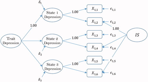
The first example considers a model for the medical illness of depression. The data ($N=323)$ used in this example are taken from Geiser (2012) and consist of six indicators of depression. In the data, $X_{1,1}$ and $X_{1,2}$ are indicators of the first-order common factor Depression State 1, $X_{1,3}$ and $X_{1,4}$ are indicators of the first-order common factor Depression State 2, and $X_{1,5}$ and $X_{1,6}$ are indicators of the first-order common factor Depression State 3. The three factors themselves are indicators of the second-order common trait factor Depression. The model additionally contains an indicator-specific factor labeled IS. Indicators $X_{1,1},$ $X_{1,2},$ $X_{1,3},$ $X_{1,5}$, and the factor Depression State 1 serve as marker variables. The path diagram illustrating the structure of the model is shown in Figure 1.

Figure 1. Geiser (2012).

Results of the estimation are presented in Table 1. As seen from the table, the number of iterations and function evaluations is (It, Fe) $=$ (23, 375) for SNLLS and (It, Fe) $=$ (145, 5439) for NLLS. As expected, the required computational load for minimizing $F\left({\mathit{\vartheta }}_{\beta ,\gamma ,\lambda }\right)$ w.r.t. ${\mathit{\vartheta }}_{\beta ,\gamma ,\lambda }$ is far less than the required load for minimizing $F\left(\mathit{\vartheta }\right)$ w.r.t. $\mathit{\vartheta }.$ Figure 2 shows the convergence profiles for the two implementations. From the figure, it is clear that the SNLLS objective function $F\left({\mathit{\vartheta }}_{\beta ,\gamma ,\lambda }\right)$ starts at a point much closer to its minimum of 0.0109 than what is seen for the NLLS objective function $F\left(\mathit{\vartheta }\right).$ In terms of estimation time, the mean time is 0.0334 sec. for SNLLS and 0.1408 sec. for NLLS. Thus, SNLLS is faster by a factor of 0.1408/0.0334 $=$ 4.2153. The results in this example clearly suggest that the SNLLS implementation is numerically more efficient than the standard NLLS implementation.

Figure 2. Convergence profile, Geiser (2012).

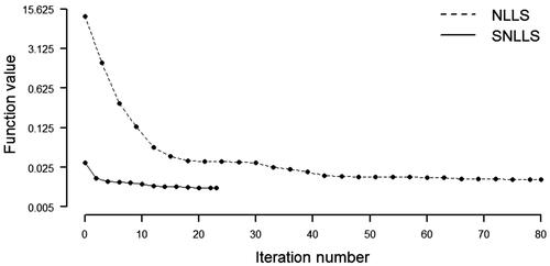
Table 1. Timing results, Geiser (2012).

	SNLLS	NLLS
Mean est. time (in sec.)	0.0334	0.1408
Median est. time in (sec.)	0.0323	0.1393
Standard dev. est. time in (sec.)	0.0047	0.0067
Minimum objective func. value	0.0109	0.0109
Number of iterations (It)	23	145
Number func. evaluations (Fe)	375	5439
$t_{{\sigma }_{\xi ,\delta ,ϵ}}/t_{{\mathit{\vartheta }}_{\beta ,\gamma ,\lambda }}$	1.57	1.57

4.2. Example 2

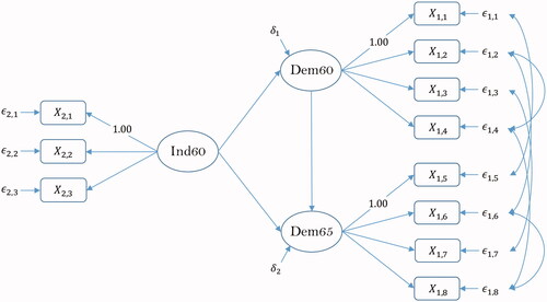
The second example considers a model for industrialization and political democracy. The model is taken from Bollen (1989), and has been used extensively in books, tutorials, etc. The data consist of 11 indicators of industrialization and political democracy for 75 countries ($N=75).$ In the data, $X_{1,1},\dots ,X_{1,4}$ are indicators of the common factor Political Democracy at time 1 (1960), $X_{1,5},\dots ,X_{1,8}$ are indicators of the common factor Political Democracy at time 2 (1965) and $X_{2,1},\dots ,X_{2,3}$ are indicators of the common factor Industrialization at time 1 (1960). Due to the repeated measurement design, the unique factors belonging to $X_{1,i}$ and $X_{1,i+4}$ for $i=1,\dots ,4$ are set to correlate. Additionally, the unique factors belonging to $X_{1,i}$ and $X_{1,i+2}$ for $i=2, 6$ are set to correlate. Indicators $X_{1,1},$ $X_{1,5}$ and $X_{2,1}$ serve as marker variables. The path diagram of the model is shown in Figure 3.

Figure 3. Bollen (1989).

Results of the estimation are presented in Table 2. The results in this example generally confirm the results from the previous example. In this case, the number of iterations and function evaluations are (It, Fe) $=$ (26, 759) for SNLLS and (It, Fe) $=$ (230, 14742) for NLLS. Figure 4 shows the convergence profiles for the two implementations. The patterns in the figure resemble those in Figure 2. Considering the estimation time, the mean time is 0.1257 sec. for SNLLS and 0.8263 sec. for NLLS. In this case, SNLLS proves to be faster by a factor of 0.8263/0.1257 $=$ 6.5736.

Figure 4. Convergence profile, Bollen (1989).

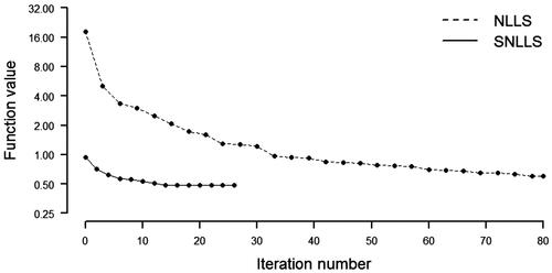
Table 2. Timing results, Bollen (1989).

	SNLLS	NLLS
Mean est. time (in sec.)	0.1257	0.8263
Median est. time in (sec.)	0.1244	0.8246
Standard dev. est. time in (sec.)	0.0106	0.0182
Minimum objective func. value	0.4858	0.4858
Number of iterations (It)	26	230
Number func. evaluations (Fe)	759	14742
$t_{{\sigma }_{\mathrm{\xi },\mathrm{\delta },ϵ}}/t_{{\mathit{\vartheta }}_{\beta ,\gamma ,\lambda }}$	1.82	1.82

5. Concluding Remarks

In this study, we have presented an SNLLS implementation of the MD objective function for estimating SEMs. The outlined framework includes all necessary expressions for applying SNLLS, and represents a generalization of previously known results. Using examples from the SEM literature, we demonstrated that the computational load of applying SNLLS is considerably less than that of applying NLLS. Another benefit of SNLLS is that fewer starting values are required, which may mitigate potential problems due to the somewhat arbitrary choice of starting values for the covariance parameters.

The present work may have several interesting extensions. First, as shown by research, SNLLS may hold a potential for improving numerical performance in situations in which the estimation problem is ill-conditioned. Thus, an interesting case for future research would be to compare the numerical performance of SNLLS and NLLS under more challenging conditions in which the condition number of the observed covariance matrix is large. Second, the SNLLS implementation is not yet available for maximum likelihood (ML) estimation. Some initial work on this topic is underway. This work, combined with the previous point, may lead to an improved implementation of the ML estimator when applied to SEMs.

Appendices

A. Deriving L and K  

Let $\mathit{x}$ be an arbitrary $p\times 1$ random vector, and let ${\mathit{\Sigma }}_x=\left\{{\sigma }_{i,j}\right\}$ be the associated $p\times p$ covariance matrix. The purpose of the following presentation is to introduce an algebraic framework that facilitates eliminating the redundancy originating from the structure of ${\mathit{\Sigma }}_x.$ To do so, let ${\mathit{K}}_x$ be a matrix such that (A1) $${\mathit{\sigma }}_x={\mathit{K}}_x^{T}vec\left({\mathit{\Sigma }}_x\right),$$(A1) where ${\mathit{\sigma }}_x$ is a covariance vector containing the nonredundant elements of ${\mathit{\Sigma }}_x$ and ${\mathit{K}}_x$ is a matrix obtained by (A2) $${\mathit{K}}_x={\mathit{L}}_x{\left({\mathit{L}}_x^T{\mathit{L}}_x\right)}^{-1}.$$(A2) In this expression, ${\mathit{L}}_x$ is a selection matrix (i.e., a matrix composed of zeros and ones).

Below, we propose a rather general framework that applies to any structure characterizing ${\mathit{\Sigma }}_x.$ Before presenting some examples on how to obtain ${\mathit{L}}_x,$ it is necessary to introduce some additional notation. Let $\mathit{E}\left(u,v\right)=\left\{e_{i,j}\left(u,v\right)\right\}$ denote a $p\times p$ matrix (for $i,j=1,\dots ,p$) with elements (A3) $$e_{i,j}\left(u,v\right)=\{\begin{array}{cc} 1& if {\sigma }_{i,j}={\sigma }_{u,v}\\ 0& o\mathit{therwise}\end{array} .$$(A3) Next, we demonstrate how to obtain ${\mathit{L}}_x$ for two standard cases and one case specialized for the SNLLS implementation.

Case 1:

As a start, consider the case in which ${\mathit{\Sigma }}_x$ is symmetric and no other restrictions are placed on its elements. The covariance vector containing the $2^{-1}p\left(p+1\right)$ nonredundant elements of ${\mathit{\Sigma }}_x$ is (A4) $${\mathit{\sigma }}_x={\left({\sigma }_{1,1} \dots {\sigma }_{p,1} {\sigma }_{2,2} \dots {\sigma }_{p,2} {\sigma }_{3,3} \dots \dots {\sigma }_{p,p}\right)}^T.$$(A4) Applying (A3), the matrix ${\mathit{L}}_{\mathit{x}}$ is formed by horizontally concatenating $2^{-1}p\left(p+1\right)$ vectors using (A5) $$\begin{array}{c}{\mathit{L}}_x=(\mathit{vec}\left(\mathit{E}\left(1,1\right)\right) \dots \mathit{vec}\left(\mathit{E}\left(p,1\right)\right) \mathit{vec}\left(\mathit{E}\left(2,2\right)\right) \dots \mathit{vec}\left(\mathit{E}\left(p,2\right)\right)\\ \mathit{vec}\left(\mathit{E}\left(3,3\right)\right) \dots \dots \mathit{vec}\left(\mathit{E}\left(p,p\right)\right)).\end{array}$$(A5)

Case 2:

Now, consider the case in which ${\mathit{\Sigma }}_x$ is diagonal. The covariance vector containing the $p$ nonredundant elements of ${\mathit{\Sigma }}_x$ is given by (A6) $${\mathit{\sigma }}_x={\left({\sigma }_{1,1} {\sigma }_{2,2} \dots {\sigma }_{p,p}\right)}^T.$$(A6) The matrix ${\mathit{L}}_x$ is now formed by horizontally concatenating $p$ vectors (A7) $${\mathit{L}}_x=\left(\mathit{vec}\left(\mathit{E}\left(1,1\right)\right) \mathit{vec}\left(\mathit{E}\left(2,2\right)\right) \dots \mathit{vec}\left(\mathit{E}\left(p,p\right)\right)).\right.$$(A7) Before introducing the third and final case, it is necessary to expand the notation. Let ${\mathit{x}}_1$ and ${\mathit{x}}_2$ be respectively $p_1\times 1$ and $p_2\times 1$ random vectors, and let $\mathit{x}$ be a $p=p_1+p_2$ dimensional column vector obtained by stacking ${\mathit{x}}_1$ and ${\mathit{x}}_2$ in the following way (A8) $$\mathit{x}={\left({\mathit{x}}_1^T {\mathit{x}}_2^T\right)}^T.$$(A8) The associated p × p covariance matrix is given by (A9) $${\mathit{\Sigma }}_x=\left(\begin{array}{cc}\underset{\left(p_1\times p_1\right)}{{\mathit{\Sigma }}_{x_1}}& \underset{\left(p_1\times p_2\right)}{{\mathit{\Sigma }}_{x_2,x_1}^T}\\ \underset{\left(p_2\times p_1\right)}{{\mathit{\Sigma }}_{x_2,x_1}}& \underset{\left(p_2\times p_2\right)}{{\mathit{\Sigma }}_{x_2}}\end{array}\right).$$(A9)

Case 3:

As in the first case, suppose that no other restrictions, apart from symmetry, are placed on the elements of ${\mathit{\Sigma }}_x.$ Let the covariance vector containing the $2^{-1}p\left(p+1\right)$ nonredundant elements of ${\mathit{\Sigma }}_x$ be given by (A10) $${\stackrel{\sim }{\mathit{\sigma }}}_x={\left({\mathit{\sigma }}_{x_1}^T {\mathit{\sigma }}_{x_2}^T {\mathit{\sigma }}_{x_2,x_1}^T\right)}^T,$$(A10) where (A11) $${\mathit{\sigma }}_{x_1}={\left({\sigma }_{1,1}\mathrm{ }\dots \mathrm{ }{\sigma }_{p_1,1}\mathrm{ }{\sigma }_{2,2}\mathrm{ }\dots \mathrm{ }{\sigma }_{p_1,2}\mathrm{ }{\sigma }_{3,3}\mathrm{ }\dots \mathrm{ }\dots \mathrm{ }{\sigma }_{p_1,p_1}\right)}^T,$$(A11) (A12) $${\mathit{\sigma }}_{x_2}={\left({\sigma }_{p_1+1,p_1+1}\mathrm{ }\dots \mathrm{ }{\sigma }_{p,p_1+1}\mathrm{ }{\sigma }_{p_1+2,p_1+2}\mathrm{ }\dots \mathrm{ }{\sigma }_{p,p_1+2}\mathrm{ }{\sigma }_{p_1+3,p_1+3}\mathrm{ }\dots \mathrm{ }\dots \mathrm{ }{\sigma }_{p,p}\right)}^T,$$(A12) (A13) $${\mathit{\sigma }}_{x_2,x_1}={\left({\sigma }_{p_1+1,1}\mathrm{ }\dots \mathrm{ }{\sigma }_{p,1}\mathrm{ }{\sigma }_{p_1+1,2}\mathrm{ }\dots \mathrm{ }{\sigma }_{p,2}\mathrm{ }{\sigma }_{p_1+1,3}\mathrm{ }\dots \mathrm{ }\dots \mathrm{ }{\sigma }_{p,p_1}\right)}^T.$$(A13)

Construct a matrix ${\stackrel{\sim }{\mathit{L}}}_x$ by horizontally concatenating three matrices (A14) $${\stackrel{\sim }{\mathit{L}}}_x=({({\stackrel{\sim }{\mathit{L}}}_x)}_{1,1} {({\stackrel{\sim }{\mathit{L}}}_x)}_{1,2} {({\stackrel{\sim }{\mathit{L}}}_x)}_{1,3}),$$(A14) where the submatrices are given by (A15) $$\begin{array}{c}{({\stackrel{\sim }{\mathit{L}}}_x)}_{1,1}=(\mathit{vec}\left(\mathit{E}\left(1,1\right)\right)\mathrm{ }\dots \mathrm{ }\mathit{vec}\left(\mathit{E}\left(p_1,1\right)\right)\mathrm{ }\mathit{vec}\left(\mathit{E}\left(2,2\right)\right)\mathrm{ }\dots \mathrm{ }\mathit{vec}\left(\mathit{E}\left(p_1,2\right)\right)\\ \mathrm{ }\mathit{vec}\left(\mathit{E}\left(3,3\right)\right)\mathrm{ }\dots \mathrm{ }\dots \mathrm{ }\mathit{vec}\left(\mathit{E}\left(p_1,p_1\right)\right)),\end{array}\mathrm{ }$$(A15) (A16) $$\begin{array}{c}{({\stackrel{\sim }{\mathit{L}}}_x)}_{1,2}=(\mathit{vec}\left(\mathit{E}\left(p_1+1,p_1+1\right)\right)\mathrm{ }\dots \mathrm{ }\mathit{vec}\left(\mathit{E}\left(p,p_1+1\right)\right)\\ vec\left(\mathit{E}\left(p_1+2,p_1+2\right)\right)\mathrm{ }\dots \mathrm{ }\mathit{vec}\left(\mathit{E}\left(p,p_1+2\right)\right)\\ \mathrm{ }\mathit{vec}\left(\mathit{E}\left(p_1+3,p_1+3\right)\right)\mathrm{ }\dots \mathrm{ }\dots \mathrm{ }\mathit{vec}\left(\mathit{E}\left(p,p\right)\right)),\end{array}\mathrm{ }$$(A16) (A17) $$\begin{array}{c}{({\stackrel{\sim }{\mathit{L}}}_x)}_{1,3}=(\mathit{vec}\left(\mathit{E}\left(p_1+1,1\right)\right)\mathrm{ }\dots \mathrm{ }\mathit{vec}\left(\mathit{E}\left(p,1\right)\right)\mathrm{ }\mathit{vec}\left(\mathit{E}\left(p_1+1,2\right)\right)\mathrm{ }\dots \mathrm{ }\mathit{vec}\left(\mathit{E}\left(p,2\right)\right)\\ \mathit{vec}\left(\mathit{E}\left(p_1+1,3\right)\right)\mathrm{ }\dots \mathrm{ }\dots \mathrm{ }\mathit{vec}(\mathit{E}\left(p,p_1\right))).\end{array}\mathrm{ }\mathrm{ }$$(A17) The number of columns in (A15(A15) $$\begin{array}{c}{({\stackrel{\sim }{\mathit{L}}}_x)}_{1,1}=(\mathit{vec}\left(\mathit{E}\left(1,1\right)\right)\mathrm{ }\dots \mathrm{ }\mathit{vec}\left(\mathit{E}\left(p_1,1\right)\right)\mathrm{ }\mathit{vec}\left(\mathit{E}\left(2,2\right)\right)\mathrm{ }\dots \mathrm{ }\mathit{vec}\left(\mathit{E}\left(p_1,2\right)\right)\\ \mathrm{ }\mathit{vec}\left(\mathit{E}\left(3,3\right)\right)\mathrm{ }\dots \mathrm{ }\dots \mathrm{ }\mathit{vec}\left(\mathit{E}\left(p_1,p_1\right)\right)),\end{array}\mathrm{ }$$(A15) ), (A16(A16) $$\begin{array}{c}{({\stackrel{\sim }{\mathit{L}}}_x)}_{1,2}=(\mathit{vec}\left(\mathit{E}\left(p_1+1,p_1+1\right)\right)\mathrm{ }\dots \mathrm{ }\mathit{vec}\left(\mathit{E}\left(p,p_1+1\right)\right)\\ vec\left(\mathit{E}\left(p_1+2,p_1+2\right)\right)\mathrm{ }\dots \mathrm{ }\mathit{vec}\left(\mathit{E}\left(p,p_1+2\right)\right)\\ \mathrm{ }\mathit{vec}\left(\mathit{E}\left(p_1+3,p_1+3\right)\right)\mathrm{ }\dots \mathrm{ }\dots \mathrm{ }\mathit{vec}\left(\mathit{E}\left(p,p\right)\right)),\end{array}\mathrm{ }$$(A16) ), and (A17(A17) $$\begin{array}{c}{({\stackrel{\sim }{\mathit{L}}}_x)}_{1,3}=(\mathit{vec}\left(\mathit{E}\left(p_1+1,1\right)\right)\mathrm{ }\dots \mathrm{ }\mathit{vec}\left(\mathit{E}\left(p,1\right)\right)\mathrm{ }\mathit{vec}\left(\mathit{E}\left(p_1+1,2\right)\right)\mathrm{ }\dots \mathrm{ }\mathit{vec}\left(\mathit{E}\left(p,2\right)\right)\\ \mathit{vec}\left(\mathit{E}\left(p_1+1,3\right)\right)\mathrm{ }\dots \mathrm{ }\dots \mathrm{ }\mathit{vec}(\mathit{E}\left(p,p_1\right))).\end{array}\mathrm{ }\mathrm{ }$$(A17) ) is $2^{-1}{p}_1\left(p_1+1\right),$ $2^{-1}{p}_2\left(p_2+1\right)$ and $p_2\times p_1,$ respectively.

B. Deriving $\mathit{G}\left({\mathit{\vartheta }}_{\beta ,}{ }_{\gamma ,}{ }_{\lambda }\right)$

The derivation below uses the following matrix identity (B1) $$\mathit{vec}\left(\mathit{ABC}\right)=\left({\mathit{C}}^T⨂\mathit{A}\right)vec\left(\mathit{B}\right),$$(B1) where $\mathit{A},$ $\mathit{B}$, and $\mathit{C}$ are matrices of compatible sizes. In addition, we make use of the following relations (B2) $$\begin{array}{c}vec\left({\mathit{\Sigma }}_{\xi }\right)={\mathit{L}}_{\xi }{\mathit{\sigma }}_{\xi }, \mathit{vec}\left({\mathit{\Sigma }}_{\delta }\right)={\mathit{L}}_{\delta }{\mathit{\sigma }}_{\delta }, \mathit{vec}\left({\mathit{\Sigma }}_{{ϵ}_1}\right)={\mathit{L}}_{{ϵ}_1}{\mathit{\sigma }}_{{ϵ}_1},\\ vec\left({\mathit{\Sigma }}_{{ϵ}_2}\right)={\mathit{L}}_{{\mathit{ϵ}}_2}{\mathit{\sigma }}_{{ϵ}_2}.\end{array}$$(B2) The model-implied covariance matrix is (B3) $$\begin{array}{c}{\mathit{\Sigma }}_x\left(\mathit{\vartheta }\right)=\left(\begin{array}{cc}{\mathit{\Sigma }}_{x_1}\left(\mathit{\vartheta }\right)& {\mathit{\Sigma }}_{x_2,x_1}^{\mathit{T}}\left(\mathit{\vartheta }\right)\\ {\mathit{\Sigma }}_{x_2,x_1}\left(\mathit{\vartheta }\right)& {\mathit{\Sigma }}_{x_2}\left(\mathit{\vartheta }\right)\end{array}\right)\\ =\left(\begin{array}{cc}{\mathit{\Lambda }}_1\mathit{H}\left(\mathit{\Gamma }{\mathit{\Sigma }}_{\xi }{\mathit{\text{Γ}}}^T+{\mathit{\Sigma }}_{\delta }\right){\mathit{H}}^T{\mathit{\Lambda }}_1^{\mathit{T}}+{\mathit{\Sigma }}_{{ϵ}_1}& {\mathit{\Lambda }}_1\mathit{H}\mathit{\Gamma }{\mathit{\Sigma }}_{\xi }{\mathit{\Lambda }}_2^T+{\mathit{\Sigma }}_{{\mathit{ϵ}}_2,{ϵ}_1}^T\\ {\mathit{\Lambda }}_2{\mathit{\Sigma }}_{\xi }{\mathit{\Gamma }}^T{\mathit{H}}^T{\mathit{\Lambda }}_1^T+{\mathit{\Sigma }}_{{ϵ}_2,{ϵ}_1}& {\mathit{\Lambda }}_2{\mathit{\Sigma }}_{\xi }{\mathit{\Lambda }}_2^T+{\mathit{\Sigma }}_{{ϵ}_2}\end{array}\right)\\ =\left(\begin{array}{cc}{\mathit{\Lambda }}_1\mathit{H}\mathit{\Gamma }{\mathit{\Sigma }}_{\xi }{\mathit{\Gamma }}^T{\mathit{H}}^T{\mathit{\Lambda }}_1^T+{\mathit{\Lambda }}_1\mathit{H}{\mathit{\Sigma }}_{\delta }{\mathit{H}}^T{\mathit{\Lambda }}_1^T+{\mathit{\Sigma }}_{{ϵ}_1}& {\mathit{\Lambda }}_1\mathit{H}\mathit{\Gamma }{\mathit{\Sigma }}_{\xi }{\mathit{\Lambda }}_2^T+{\mathit{\Sigma }}_{{ϵ}_2,{ϵ}_1}^T\\ {\mathit{\Lambda }}_2{\mathit{\Sigma }}_{\xi }{\mathit{\Gamma }}^T{\mathit{H}}^T{\mathit{\Lambda }}_1^T+{\mathit{\Sigma }}_{{ϵ}_2,{ϵ}_1}& {\mathit{\Lambda }}_2{\mathit{\Sigma }}_{\xi }{\mathit{\Lambda }}_2^T+{\mathit{\Sigma }}_{{ϵ}_2}\end{array}\right).\end{array}$$(B3) Applying SNLLS, the key is to express the model-implied covariance vector using the form (B4) $$\begin{array}{c}{\stackrel{\sim }{\mathit{\sigma }}}_x\left(\mathit{\vartheta }\right)={\left({\mathit{\sigma }}_{x_1}^T\left(\mathit{\vartheta }\right)\mathrm{ }{\mathit{\sigma }}_{x_2}^T\left(\mathit{\vartheta }\right)\mathrm{ }{\mathit{\sigma }}_{x_2,x_1}^T\left(\mathit{\vartheta }\right)\right)}^T\\ :=\mathit{G}\left({\mathit{\vartheta }}_{\beta ,\gamma ,\lambda }\right){\mathit{\sigma }}_{\xi ,\delta ,ϵ}.\end{array}$$(B4) To do so, it is necessary to vectorize the individual blocks of (B3). Starting with the block ${\mathit{\Sigma }}_{x_1}\left(\mathit{\vartheta }\right),$ we have (B5) $$\begin{array}{l}{\mathit{\sigma }}_{x_1}\left(\mathit{\vartheta }\right)={\mathit{K}}_{x_1}^{T}vec\left({\mathit{\Sigma }}_{x_1}\left(\mathit{\vartheta }\right)\right)\\ ={\mathit{K}}_{x_1}^{T}vec\left({\mathit{\Lambda }}_1\mathit{H}\mathit{\Gamma }{\mathit{\Sigma }}_{\xi }{\mathit{\Gamma }}^{\mathit{T}}{\mathit{H}}^{\mathit{T}}{\mathit{\Lambda }}_1^{\mathit{T}}\right)+{\mathit{K}}_{x_1}^{T}vec\left({\mathit{\Lambda }}_1\mathit{H}{\mathit{\Sigma }}_{\mathit{\delta }}{\mathit{H}}^{\mathit{T}}{\mathit{\Lambda }}_1^{\mathit{T}}\right)+{ \mathit{K}}_{x_1}^{T}vec\left({\mathit{\Sigma }}_{{\mathit{ϵ}}_1}\right)\\ ={\mathit{K}}_{x_1}^T\left({\mathit{\Lambda }}_1\mathit{H}\mathit{\Gamma }\otimes {\mathit{\Lambda }}_1\mathit{H}\mathit{\Gamma }\right)vec\left({\mathit{\Sigma }}_{\xi }\right)+{\mathit{K}}_{x_1}^T\left({\mathit{\Lambda }}_1\mathit{H}\otimes {\mathit{\Lambda }}_1\mathit{H}\right)vec\left({\mathit{\Sigma }}_{\delta }\right)+{\mathit{K}}_{x_1}^{T}vec\left({\mathit{\Sigma }}_{{\mathit{ϵ}}_1}\right).\\ \end{array}$$(B5) Using (B1(B1) $$\mathit{vec}\left(\mathit{ABC}\right)=\left({\mathit{C}}^T⨂\mathit{A}\right)vec\left(\mathit{B}\right),$$(B1) ) and (B2(B2) $$\begin{array}{c}vec\left({\mathit{\Sigma }}_{\xi }\right)={\mathit{L}}_{\xi }{\mathit{\sigma }}_{\xi }, \mathit{vec}\left({\mathit{\Sigma }}_{\delta }\right)={\mathit{L}}_{\delta }{\mathit{\sigma }}_{\delta }, \mathit{vec}\left({\mathit{\Sigma }}_{{ϵ}_1}\right)={\mathit{L}}_{{ϵ}_1}{\mathit{\sigma }}_{{ϵ}_1},\\ vec\left({\mathit{\Sigma }}_{{ϵ}_2}\right)={\mathit{L}}_{{\mathit{ϵ}}_2}{\mathit{\sigma }}_{{ϵ}_2}.\end{array}$$(B2) ), it follows that (B6) $$\begin{array}{c}{\mathit{\sigma }}_{x_1}\left(\mathit{\vartheta }\right)={\mathit{K}}_{x_1}^T\left({\mathit{\Lambda }}_1\mathit{H}\mathit{\Gamma }\otimes {\mathit{\Lambda }}_1\mathit{H}\mathit{\Gamma }\right){\mathit{L}}_{\xi }{\mathit{\sigma }}_{\xi }+{\mathit{K}}_{x_1}^T\left({\mathit{\Lambda }}_1\mathit{H}\otimes {\mathit{\Lambda }}_1\mathit{H}\right){\mathit{L}}_{\delta }{\mathit{\sigma }}_{\delta }+{\mathit{K}}_{x_1}^T{\mathit{L}}_{{ϵ}_1}{\mathit{\sigma }}_{{ϵ}_1}\\ =\left({\mathit{K}}_{x_1}^T\left({\mathit{\Lambda }}_1\mathit{H}\mathit{\Gamma }\otimes {\mathit{\Lambda }}_1\mathit{H}\mathit{\Gamma }\right){\mathit{L}}_{\xi }\mathrm{ }{\mathit{K}}_{x_1}^T\left({\mathit{\Lambda }}_1\mathit{H}\otimes {\mathit{\Lambda }}_1\mathit{H}\right){\mathit{L}}_{\delta }\mathrm{ }{\mathit{K}}_{x_1}^T{\mathit{L}}_{{ϵ}_1}\mathrm{ }\mathbf{0}\mathrm{ }\mathbf{0}\right){\mathit{\sigma }}_{\xi ,\delta ,ϵ}.\end{array}$$(B6) Next, we consider the block ${\mathit{\Sigma }}_{x_2}\left(\mathit{\vartheta }\right).$ Using the same procedure as before, we have (B7) $$\begin{array}{l}{\mathit{\sigma }}_{x_2}\left(\mathit{\vartheta }\right)={\mathit{K}}_{x_2}^{T}vec\left({\mathit{\Sigma }}_{x_2}\left(\mathit{\vartheta }\right)\right)\\ ={\mathit{K}}_{x_2}^{T}vec\left({\mathit{\Lambda }}_2{\mathit{\Sigma }}_{\xi }{\mathit{\Lambda }}_2^T\right)+{\mathit{K}}_{x_2}^{T}vec\left({\mathit{\Sigma }}_{{ϵ}_2}\right)\\ \begin{array}{c}={\mathit{K}}_{x_2}^T\left({\mathit{\Lambda }}_2\otimes {\mathit{\Lambda }}_2\right)vec\left({\mathit{\Sigma }}_{\xi }\right)+{\mathit{K}}_{x_2}^{T}vec\left({\mathit{\Sigma }}_{{ϵ}_2}\right)\\ \begin{array}{c}={\mathit{K}}_{x_2}^T\left({\mathit{\Lambda }}_2\otimes {\mathit{\Lambda }}_2\right){\mathit{L}}_{\xi }{\mathit{\sigma }}_{\xi }+{\mathit{K}}_{x_2}^T{\mathit{L}}_{{ϵ}_2}{\mathit{\sigma }}_{{ϵ}_2}\\ =\left({\mathit{K}}_{x_2}^T\left({\mathit{\Lambda }}_2\otimes {\mathit{\Lambda }}_2\right){\mathit{L}}_{\xi }\mathrm{ }\mathbf{0}\mathrm{ }\mathbf{0}\mathrm{ }{\mathit{K}}_{x_2}^T{\mathit{L}}_{{ϵ}_2}\mathrm{ }\mathbf{0}\right){\mathit{\sigma }}_{\xi ,\delta ,ϵ}.\end{array}\end{array}\end{array}$$(B7) Finally, for the block ${\mathit{\Sigma }}_{x_2,x_1}\left(\mathit{\vartheta }\right),$ it follows that (B8) $$\begin{array}{l}{\mathit{\sigma }}_{x_2,x_1}\left(\mathit{\vartheta }\right)=\mathit{vec}\left({\mathit{\Sigma }}_{x_2,x_1}\left(\mathit{\vartheta }\right)\right)\\ =\mathit{vec}\left({\mathit{\Lambda }}_2{\mathit{\Sigma }}_{\xi }{\mathit{\Gamma }}^T{\mathit{H}}^T{\mathit{\Lambda }}_1^T\right)+\mathit{vec}\left({\mathit{\Sigma }}_{{ϵ}_2,{ϵ}_1}\right)\\ \begin{array}{c}=\left({\mathit{\Lambda }}_1\mathit{H}\mathit{\Gamma }\otimes {\mathit{\Lambda }}_2\right)vec\left({\mathit{\Sigma }}_{\xi }\right)+\mathit{vec}\left({\mathit{\Sigma }}_{{ϵ}_2,{ϵ}_1}\right)\\ =\left({\mathit{\Lambda }}_1\mathit{H}\mathit{\Gamma }\otimes {\mathit{\Lambda }}_2\right){\mathit{L}}_{\xi }{\mathit{\sigma }}_{\xi }+{\mathit{\sigma }}_{{ϵ}_2,{ϵ}_1}\\ =\left(\left({\mathit{\Lambda }}_1\mathit{H}\mathit{\Gamma }\otimes {\mathit{\Lambda }}_2\right){\mathit{L}}_{\xi }\mathrm{ }\mathbf{0}\mathrm{ }\mathbf{0}\mathrm{ }\mathbf{0}\mathrm{ }\mathit{I}\right){\mathit{\sigma }}_{\xi ,\delta ,ϵ}.\end{array}\end{array}$$(B8) Putting the pieces together, we obtain (B9) $$\left(\begin{array}{c}{\mathit{\sigma }}_{x_1}\left(\mathit{\vartheta }\right)\\ {\mathit{\sigma }}_{x_2}\left(\mathit{\vartheta }\right)\\ {\mathit{\sigma }}_{x_2,x_1}\left(\mathit{\vartheta }\right)\end{array}\right)=\left(\begin{array}{ccccc}{\mathit{K}}_{x_1}^T\left({\mathit{\Lambda }}_1\mathit{H}\mathit{\Gamma }\otimes {\mathit{\Lambda }}_1\mathit{H}\mathit{\Gamma }\right){\mathit{L}}_{\xi }& {\mathit{K}}_{x_1}^T\left({\mathit{\Lambda }}_1\mathit{H}\otimes {\mathit{\Lambda }}_1\mathit{H}\right){\mathit{L}}_{\delta }& {\mathit{K}}_{x_1}^T{\mathit{L}}_{{ϵ}_1}& \mathbf{0}& \mathbf{0}\\ {\mathit{K}}_{x_2}^T\left({\mathit{\Lambda }}_2\otimes {\mathit{\Lambda }}_2\right){\mathit{L}}_{\xi }& \mathbf{0}& \mathbf{0}& {\mathit{K}}_{x_2}^T{\mathit{L}}_{{ϵ}_2}& \mathbf{0}\\ \left({\mathit{\Lambda }}_1\mathit{H}\mathit{\Gamma }\otimes {\mathit{\Lambda }}_2\right){\mathit{L}}_{\xi }& \mathbf{0}& \mathbf{0}& \mathbf{0}& \mathit{I}\end{array}\right) \times {\mathit{\sigma }}_{\xi ,\delta ,ϵ}.$$(B9)

References

- Bollen, K. A. (1989). Structural equations with latent variables. Wiley.
- Dattner, I., Ship, H., & Voit, E. O. (2020). Separable nonlinear least-squares parameter estimation for complex dynamic systems. Complexity, 2020, 1–11. https://doi.org/10.1155/2020/6403641
- Geiser, C. (2012). Data analysis with Mplus. Guilford Press.
- Golub, G. H., & Pereyra, V. (1973). The differentiation of pseudo-inverses and nonlinear least squares problems whose variables separate. SIAM Journal on Numerical Analysis, 10, 413–432. https://doi.org/10.1137/0710036
- Golub, G. H., & Pereyra, V. (2003). Separable nonlinear least squares: The variable projection method and its applications. Inverse Problems, 19, R1–R26. https://doi.org/10.1088/0266-5611/19/2/201
- Hägglund, G. (1982). Factor analysis by instrumental variables methods. Psychometrika, 47, 209–222. https://doi.org/10.1007/BF02296276
- Kreiberg, D., Marcoulides, K., & Olsson, U. H. (2021). A faster procedure for estimating CFA models applying minimum distance estimators with a fixed weight matrix. Structural Equation Modeling: A Multidisciplinary Journal, 28, 725–739. https://doi.org/10.1080/10705511.2020.1835484
- Kreiberg, D., Söderström, T., & Yang-Wallentin, F. (2016). Errors-in-variables system identification using structural equation modeling. Automatica, 66, 218–230. https://doi.org/10.1016/j.automatica.2015.12.007
- Magnus, J. R., & Neudecker, H. (1999). Matrix differential calculus with applications in statistics and econometrics. John Wiley & Sons.
- MATLAB version R2020b. (2020). The MathWorks Inc.
- Mullen, K. M. (2008). Separable nonlinear models: Theory, implementation and applications in physics and chemistry [Ph.D. thesis]. Vrije Universiteit Amsterdam.
- R Core Team (2021). R: A language and environment for statistical computing. R Foundation for Statistical Computing. http://www.R-project.org/
- Rosseel, Y. (2012). lavaan: An R package for structural equation modeling. Journal of Statistical Software, 48, 1–36. https://doi.org/10.18637/jss.v048.i02
- Sjöberg, J., & Viberg, M. (1997). Separable non-linear least-squares minimization-possible improvements for neural net fitting. In Neural networks for signal processing VII. Proceedings of the 1997 IEEE signal processing society workshop (pp. 345–354). IEEE.
- Söderström, T., & Mossberg, M. (2011). Accuracy analysis of a covariance matching approach for identifying errors-in-variables systems. Automatica, 47, 272–282. https://doi.org/10.1016/j.automatica.2010.10.046
- Söderström, T., Mossberg, M., & Hong, M. (2009). A covariance matching approach for identifying errors-in-variables systems. Automatica, 45, 2018–2031. https://doi.org/10.1016/j.automatica.2009.05.010