Power Analysis for the Random Intercept Cross-Lagged Panel Model Using the powRICLPM R-Package

Abstract

The random intercept cross-lagged panel model (RI-CLPM) is a popular model among psychologists for studying reciprocal effects in longitudinal panel data. Although various texts and software packages have been published concerning power analyses for structural equation models (SEM) generally, none have proposed a power analysis strategy that is tailored to the particularities of the RI-CLPM. This can be problematic because mismatches between the power analysis design, the model, and reality, can negatively impact the validity of the recommended sample size and number of repeated measures. As power analyses play an increasingly important role in the preparation phase of research projects, an RI-CLPM-specific strategy for the design of a power analysis is detailed, and implemented in the R-package powRICLPM. This paper focuses on the (basic) bivariate RI-CLPM, and extensions to include constraints over time, measurement error (leading to the stable trait autoregressive trait state model), non-normal data, and bounded estimation.

Keywords:

• Power
• random intercept cross-lagged panel model
• R-package
• stable trait autoregressive trait state model

A popular model among psychologists for the analysis of panel data is the random intercept cross-lagged panel model (RI-CLPM). It was first formally introduced by Hamaker et al. (2015) as an extension of the traditional cross-lagged panel model (CLPM; Rogosa, 1980) to account for stable, between-unit differences in the data. Unlike the CLPM, the RI-CLPM separates stable, between-unit variance from fluctuating, within-unit variance: The autoregressive effects can then be interpreted as purely within-unit effects and carry-over (rather than estimates of stability of the rank-order of units, as is the case in the CLPM), and cross-lagged effects can be interpreted as the within-unit effect or “spillover” of one domain into another (Mulder & Hamaker, 2021). This feature addresses some long-standing concerns that researchers have had about panel data analysis, such as the conflation of within- and between-unit variance for studying within-unit processes, unobserved heterogeneity, and bias in the cross-lagged effects due to omitted variables (Andersen, 2021; Hamaker et al., 2015; Heise, 1970; Kenny & Zautra, 1995, 2001). The reader is referred to Usami (2021), Zyphur, Allison, et al. (2020), and Zyphur, Voelkle, et al. (2020) for an overview of how related SEM models address these concerns.

A frequently asked question by substantive researchers in relation to the RI-CLPM, is about the required sample size for detecting hypothesized effects. Such questions of statistical power are especially relevant in the design phase of a study: Underpowered study designs are more likely to result in Type II errors (i.e., incorrectly failing to reject the null-hypothesis of no effect), whereas overpowered studies (i.e., study designs with a sample size larger than necessary to find hypothesized effects) can place an unreasonable burden on the research resources (Zhang & Liu, 2018). While there are some general rules of thumb in the structural equation modeling (SEM) literature for what is regarded an adequate sample size (cf. Barrett, 2007; Jackson, 2003; Little, 2013; MacCallum et al., 1996), in practice, statistical power depends on many factors and assumptions, making it difficult to come up with a generally applicable sample size recommendation. When planning a longitudinal study, it is therefore advized to perform a power analysis that is tailored to a particular research context and research question, to find the optimal study design (Oertzen et al., 2010; Wang & Rhemtulla, 2021; Wolf et al., 2013). However, it can be challenging to design and perform such a study for researchers who are inexperienced with simulation-based power analyses, the particularities of a model, and the software required to automate the process.

This paper proposes a strategy for setting up and executing a power analysis for the RI-CLPM based on Monte Carlo simulations, and implements it in the R-package powRICLPM. Although treatments on the design and implementation of Monte Carlo studies have appeared before (cf. Lee, 2015; Muthén & Muthén, 2002; Paxton et al., 2001; Wang & Rhemtulla, 2021; Zhang & Liu, 2018), these texts are not particular to the characteristics of the RI-CLPM, or target model (mis)fit rather than specific parameters within the model. Performing a power analysis for the RI-CLPM involves numerous model-specific and complex decisions which have not been described in the literature yet. The focus of this paper is on à priori power analysis (e.g., during the planning phase of a study, or as part of a grant proposal), but the procedure can similarly be used for post hoc power analysis (e.g., at a reviewer’s request, or because dropout or nonresponse resulted in a lower-than-expected sample size; Hancock & French, 2013).

The paper is organized as follows: First, an illustrative example concerning academic amotivation is introduced that is used throughout. Second, the RI-CLPM itself is presented, as well as the factors influencing its power. Third, a 6-step power analysis strategy is laid out. Fourth, this strategy is demonstrated using the powRICLPM package and the illustrative example. Fifth, extensions of the power analysis strategy are described, including the addition of constraints on parameters over time, measurement error (thereby leading to the bivariate stable trait autoregressive trait state model by Kenny & Zautra, 2001), non-normal data, and bounded estimation. This paper concludes with limitations of the proposed procedure and a comparison with other software packages for power analysis.

1. Illustrating Example: Self-Alienation and Academic Amotivation

Suppose we are interested in the prevention of loss of academic motivation in students, and have reason to believe (based on previous research and expert opinion) that self-alienation is a driving factor herein. More specifically, we want to investigate the reciprocal effects of self-alienation X (the feeling that one does not know oneself) and academic amotivation Y (a lack of intrinsic or extrinsic motivation for pursuing academic goals) in college students over time. Unfortunately, due to time and money constraints, we are unable to design a randomized experiment in which self-alienation X is intervened on, and are therefore bound to observational data. As such, we want to use the RI-CLPM to estimate cross-lagged effects while controlling for stable, between-person differences in self-alienation and academic amotivation. Suppose further that we deem the assumptions underlying the RI-CLPM plausible, namely that the reciprocal effects between self-alienation and academic amotivation are: (a) linear; (b) constant across units (homogeneity); (c) constant across the values of our observed variables and error terms (no effect modification); (d) not affected by unobserved time-varying confounding; and (e) the error terms (approximately) follow a multivariate normal distribution (Gische & Voelkle, 2021).

Prior to the start of the data collection, we want to perform a power analysis to determine the required sample size N and number of repeated measures T for detecting potential reciprocal effects with a power level of 0.8. Planning for N and T is a matter of balance: It can be beneficial in terms of time and costs to collect an additional wave of data rather than additional participants, or vice versa, while maintaining the desired level of statistical power. Some researchers, like Winkens et al. (2006), explicitly include a “costs function” in their power analysis to determine an optimal trade-off in terms of sample size and number of repeated measures (as well as other factors).

2. The Model

Figure 1 presents an RI-CLPM for a study design with three repeated measures. Let X_it and Y_it be the observed values for self-alienation and academic amotivation for individual i at time point t, respectively. By fitting an RI-CLPM, these observed variables are decomposed into three independent components: grand means ${\mu }_{X,t}$ and ${\mu }_{Y,t}$ for each time-point, time-invariant random intercept factors $R{I}_{X,i}$ and $R{I}_{Y,i},$ and time-varying within-components $W_{X,it}$ and $W_{Y,it},$ for self-alienation and academic amotivation respectively. These decompositions are represented by (1) $$X_{it}={\mu }_{X,t}+R{I}_{X,i}+W_{X,it},$$(1) (2) $$Y_{it}={\mu }_{Y,t}+R{I}_{Y,i}+W_{Y,it}.$$(2)

Figure 1. A bivariate random intercept cross-lagged panel model with three waves of data. α_t and δ_t are autoregressive effects of W_X and W_Y, respectively. γ_t and β_t are the cross-lagged effects of $W_{X,t-1}$ on $W_{Y,t}$ and $W_{Y,t-1}$ on $W_{X,t},$ respectively. The mean structure with ${\mu }_{X,t}$ and ${\mu }_{Y,t}$ is not explicitly included here.

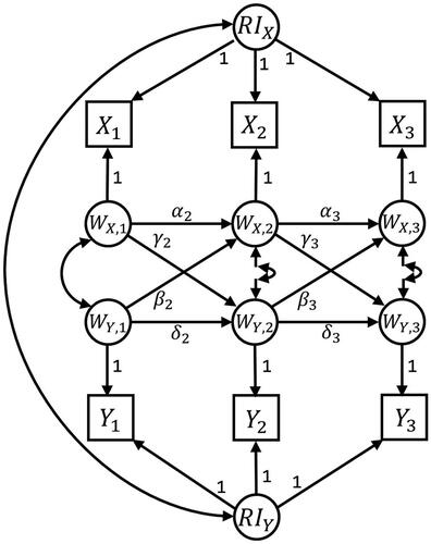
The grand means are time-specific means across all individuals, and they can be freely estimated in the model or constrained over time. The random intercepts RI_X and RI_Y are latent factors, with the observed measures for self-alienation as indicators for RI_X and the observed measures for academic amotivation for RI_Y. They capture individuals’ stable, time-invariant (i.e., for the duration of the study) deviations from the grand means ${\mu }_{X,t}$ and ${\mu }_{Y,t},$ such that the random intercept factors exclusively represent between-person variance. In the standard RI-CLPM presented here, the factor loadings of the random intercept factors are fixed at 1, implying that the size of the stable, between-person differences is invariant over time. However this may be an assumption that researchers want to check by freely estimating these factor loadings and comparing model fit (Mulder & Hamaker, 2021). Finally, the within-components $W_{X,it}$ and $W_{Y,it}$ represent the deviation of an individual at a specific time-point from the individual’s expected score based on the grand mean and the random intercept.

Next, autoregressive and cross-lagged effects are added between the within-components at subsequent waves, such that (3) $$W_{X,it}={\alpha }_t{W}_{X,i,t-1}+{\beta }_t{W}_{Y,i,t-1}+u_{it},$$(3) (4) $$W_{Y,it}={\delta }_t{W}_{Y,i,t-1}+{\gamma }_t{W}_{X,i,t-1}+v_{it},$$(4) where α_t represents the autoregressive effect of self-alienation from wave t − 1 to wave t, δ_t represents the autoregressive effect of academic amotivation from wave t − 1 to wave t, β_t is the cross-lagged effect from academic amotivation at wave t − 1 to self-alienation at wave t, and γ_t is the cross-lagged effect from self-alienation at wave t − 1 to academic amotivation at wave t. u_it and v_it are zero-mean normally distributed residuals with variances ${\sigma }_{u,t}^2$ and ${\sigma }_{v,t}^2,$ respectively, and they are allowed to covary with each other within each wave. Because the within-person variance is separated from the stable, between-person variance, the lagged effects pertain exclusively to within-person fluctuations. The autoregressive parameters α_t and δ_t can then be interpreted as carry-over or inertia (Kuppens et al., 2010; Suls et al., 1998), whereas the cross-lagged parameters β_t and γ_t represent the within-person spill-over of the one construct into the other (i.e., controlled for stable, between-person differences), and vice versa. Finally, including a covariance between the between-components RI_X and RI_Y completes the basic setup of the RI-CLPM. The model is flexible, and can be extended to include constraints over time, time-invariant and time-varying predictors and outcomes, multiple groups, multiple indicators (Mulder & Hamaker, 2021), and interactions to test for moderation (Ozkok et al., 2022).

2.1. Factors Influencing Power

Besides sample size and the number of repeated measures, there are many other factors that influence the RI-CLPM’s power to detect individual non-zero parameters.¹ It is important to carefully consider and include these in the setup of a power analysis as they can impact the validity of the power analysis results. Here, these factors are divided into two groups: Characteristics of the study design, and characteristics of the data.

Characteristics of the study design that influence statistical power are interesting because they are under control of the researcher, and can be tweaked to achieve the desired amount of power. Sample size and number of repeated measures are the two most obvious examples of such factors. Others include: (a) the significance criterion, where a larger criterion leads to a higher probability of rejecting the null-hypothesis of no effect, but also increases the probability of Type I errors (Zhang & Liu, 2018); (b) model complexity, where it has been suggested that models with fewer freely estimated parameters, for example due to imposed parameter constraints over time, have more power to detect non-null effects (Wang & Rhemtulla, 2021); and (c) in the case of a multiple-indicator RI-CLPM, the number of indicators, as the inclusion of multiple indicators allows for controlling for measurement error, thereby increasing power (Oertzen et al., 2010; Wang & Rhemtulla, 2021).

Characteristics of the data that impact power are important to consider as well. Even though these cannot be controlled by the researcher, failing to adequately represent these data characteristics in the simulated data in the power analysis can negatively affect the validity of the power analysis results. These factors include: (a) the effect size, where larger effects in the data result in larger test statistics, and thus greater power to reject the null-hypothesis of no effect (Wang & Rhemtulla, 2021); (b) non-normality, because many SEM models actually assume multivariate normal data, and non-normality then negatively impacts power (Yuan et al., 2015; Zhang 2014); (c) missing data, although some missing data patterns have a larger impact than others (Zhang & Liu, 2018); (d) the reliability of indicators, where smaller measurement error variances leads to larger power (this is also related to the impact of the use of multiple indicators on power; Oertzen et al., 2010; Wang & Rhemtulla, 2021); and (e) the proportion of between-unit variance in the observed data. This last factor warrants additional explanation as the decomposition of observed variance into independent between-unit and within-unit variance is particular to the RI-CLPM (and the stable trait autoregressive trait state model, as discussed in Section 5.2 “Measurement Error”). If a large portion of the observed variance is captured by the random intercepts, this implies that relatively little variance remains in the within-components. Consequently, point estimates of parameters at the within-unit level of the model, including the lagged effects of interest, are less certain, leading to higher standard errors and lower power. This point will be illustrated in Section 4 using the illustrative example.

3. The Power Analysis Strategy

With the illustrative example, the RI-CLPM, and the factors influencing its statistical power introduced, a strategy for RI-CLPM power analysis is presented next. Because analytical solutions to power-related questions often become intractable in realistic situations, with small sample sizes, complex models, and when the underlying assumptions of a model are not met (Bandalos & Leite, 2013; Lee, 2015), this power analysis strategy relies on Monte Carlo simulations instead (Paxton et al., 2001). In general, a Monte Carlo study is based on generating R samples from a model that is thought to represent the population of interest (referred to as the population model), and then estimating the parameters in each sample $r=1,\dots ,R.$ The parameter estimates from each sample are then collected, forming an (artificial) empirical sampling distribution for each parameter. The performance of the estimated parameters is then based on properties of this sampling distribution. In the case of a power analysis, the population model is the same as the estimated model: Here, the RI-CLPM. Sampling distribution properties of interest include the proportion of times the confidence interval for the parameter(s) of interest does not include 0 (i.e., the power), the width of the associated confidence interval(s) (i.e., the accuracy), and the mean square error (MSE). Other properties exist, like the percentage and relative bias, the standard deviation around the mean parameter estimate, and the coverage rate of the confidence interval, but are typically not the primary focus of a power analysis.

The power analysis strategy presented here contains 6 steps:

1. Determine experimental conditions of interest (e.g., with varying sample sizes, numbers of repeated measures, or proportions of between-unit variance, amongst other things).

2. Choose and/or compute population parameter values.

3. Generate data from an RI-CLPM using the population parameter values from step 2.

4. Estimate an RI-CLPM on the data generated in step 3.

5. Repeat steps 3 and 4 R times for each experimental condition.

6. Summarize the R results and compare across experimental conditions.

3.1. Step 1: Define Experimental Conditions

The first step entails determining the experimental conditions that you are interested in simulating the power for. In this context, an experimental condition is a combination of values for each factor that influences the RI-CLPM’s power, for instance, the experimental condition with a sample size of 500, 3 repeated measures, a significance criterion of 0.05, a $50:50$ proportion of within- and between-unit variance, data with a skewness of 0, etc. In an à priori power analysis, a range of experimental conditions is included, where sample sizes and numbers of repeated measures are typically varying across conditions. If none of the included experimental conditions leads to the desired amount of power, the range of experimental conditions can be extended.

The key issue here is determining what are realistic values for the factors (other than the sample size and the number of repeated measures) that make up an experimental condition. If data are generated under conditions that are not representative of empirical data, the validity of the power analysis results can be severely limited (Lee, 2015; Paxton et al., 2001). This can happen, for example, when researchers wrongly assume a $90:10$ proportion of within-:between-unit variance, whereas in reality it is approximately $50:50.$ Therefore, it is recommended to define values for these factors using theory, such that any decisions can be explained and defended. Previous studies on the same topic and expert knowledge can be important sources of information for deciding what are realistic values (Bandalos & Leite, 2013; Muthén & Muthén, 2002). When the appropriateness of certain choices are ambiguous, it might be recommendable to limit the values to conservative options: For example, a higher proportion of between-unit variance, or increased levels of non-normality. Alternatively, these factors can be allowed to vary across simulation conditions as well, rather than relying on a single (ambiguous) decision. This allows the researcher to determine what conditions are tolerable without loss of the desired power level (Bandalos & Leite, 2013).

For the illustrative example, let the sample size range from 200 to 2000 using steps of 100, and the number of repeated measures range from 3 to 5. Regarding appropriate values for the proportion of between-unit variance, Kim et al. (2018) found 56% and 59% stable, between-unit variance for self-alienation and academic amotivation, respectively, for biweekly measurements, for a total of eight weeks. However, there is likely to be some uncertainty in basing the proportion of between-unit variance on previous research because research designs and contexts are never perfectly equivalent. For example, we might think that intervals of 1 month between repeated measures better reflect the time it takes for the causal effect under study to take place (Heise, 1970; Mitchell & James, 2001), and therefore plan to take monthly measurements rather than biweekly measurements. This difference in the timing of measurements is likely to affect the proportion of between-unit variance in the collected data. Therefore, to take this uncertainty into account, a range of proportions of between-unit variance is included in the power analysis, namely 0.3, 0.5, and 0.7. Furthermore, for the sake of interpretability of this illustrative example, the traditional significance criterion of 0.05 is used to denote significance, and we assume no deviations from normality, no missing data, and no measurement error (i.e., perfect reliability of the indicators).

3.2. Step 2: Choose and/or Compute Population Parameter Values

To generate data in step 3, a population model needs to be specified that acts as a data generating mechanism. To this end, population values need to be specified for each parameter in the RI-CLPM first. In this strategy, population values need to be set for: (a) the autoregressive and cross-lagged effects (standardized); (b) the correlations between within-components; and (c) the correlation between the random intercepts. Similar to defining the experimental conditions in step 1, the key issue is to choose population parameter values that are realistic. Again, it is recommended to base these decisions on previous literature, or expert opinion. In case of uncertainty, a good strategy might be to be conservative: Pick values on the smaller side of the plausible range. Other parameters in the RI-CLPM are either computed from these population parameter values (like the residual variances and covariances of the within-components at wave 2 and further), determined based on the experimental conditions as defined in step 1 (the random intercept variances), or set to 0 because they are not of primary interest here (the mean structure).

3.2.1. Step 2.1: Within-Unit Parameters

Within-unit parameters include the autoregressive effects α_t and δ_t, cross-lagged effects β_t and γ_t, variances and covariance for the within-components at wave 1, and the residual variances and covariances for the within-components at wave 2 and further. For the lagged effects we rely on the specification of standardized effects in the population model such that the power analysis does not depend on any particular metric. Kim et al. (2018) report standardized autoregressive effects of self-alienation and academic amotivation between 0.206 and 0.266, and between 0.294 and 0.529, respectively. The standardized cross-lagged effect from self-alienation to academic amotivation was estimated to be between 0.08 and 0.104, while the reverse effect was estimated to be between 0.154 and 0.301. Our strategy is to be conservative, and as such we specify a small effect of 0.20 for the autoregressive effect of self-alienation, and a small to medium effect of 0.30 for the autoregressive effect of academic amotivation (following guidelines by Cohen, 1988). This conservative approach would imply that the population parameter values for the cross-lagged effect of self-alienation to academic amotivation are set to be extremely small (i.e., 0.08). However, such small effects are arguably not interesting in practice and it is recommended to use a cutoff value—for example 0.10 as recommended by Paxton et al. (2001)—for population parameter values. We set the cross-lagged effects to be 0.10 for the effect from self-alienation to academic amotivation, and to be 0.15 for academic amotivation to self-alienation.

For these population values to be interpreted as standardized effects, the variances of the within-components need to be 1. At the first wave, the variances can be set to 1 directly as these variables are exogenous, and their covariance (which is now also the correlation) is set to 0.26, as reported by Kim et al. (2018). However, setting the variance of the within-components at wave 2 and further is more involved because these variables are endogenous. Hence, only the variances and covariance of the residuals can be set directly, rather than the variances of the within-components themselves. Taking the within-components of academic amotivation and self-alienation at wave 2 as an example, it can be shown using the path-tracing rules that their variances are a function of the variance they “inherit” from their predictors (the within-components of academic amotivation and self-alienation at the first wave), as well as the variance from their residuals (see Appendix A for details). Therefore, we must compute how much variance the residuals should have such that, together with the variance from their predictors, the variance of the within-components add up to 1.

The residual variances and covariance can be expressed as a function of the population values for the lagged effects and the correlations between the within-components (Kim & Nelson, 1999), as derived in Appendix B. Using this relationship, the residual variances and residual covariance for a wave t, given the lagged effects and the correlation between the within-components at the previous wave $t-1,$ can be computed such that it results in a variance of 1 for the within-components at wave t. For our example, this results in a residual variance of the within-component of self-alienation of 0.9219, a residual variance of the within-component of academic amotivation of 0.8844, and a residual covariance of 0.1755 at wave 2. Under the assumption of stationarity, whereby the lagged effects and the variances of and correlations between the within-components do not change over time, the residual variances and the residual covariance similarly apply to the within-components at wave 3 and further, ensuring that all within-components have a variance of 1, and that the population lagged effects can be interpreted as standardized effects at each time point.

3.2.2. Step 2.2: Between-Unit Parameters

Next, the population parameter values for the between-unit parameters need to be set, including the variances of, and covariance between the random intercepts. As the variances of the within-components are designed to be 1, the ratio of between- and within-unit variance is determined by the variance of the random intercepts: Setting the random intercept variances to 1 implies a 50% between- and 50% within-unit variance, while setting the random intercept variance to 3 leads to 75% between- and 25% within-unit variance in the observed variables. The proportion of between-unit variance is already chosen in step 1, so the exact population value of the random intercept variances can simply be computed from this. Finally, along the lines of Kim et al. (2018) we set the correlation between the random intercepts to be 0.35.

Optionally, the means can be set in the population model. While this can be of interest in the case of a multiple indicator RI-CLPM, the mean structure is typically not of (primary) interest in any basic RI-CLPM. In the former case, it is recommended to test if strong measurement invariance over time holds and therefore researchers should constrain the factor loadings and intercepts/means over time. As this is not of interest in the illustrative example, the mean structure is ignored here and the grand means are set to 0, ${\mu }_{X,t}={\mu }_{Y,t}=0.$

3.3. Steps 3–5: Generate Data, Estimate RI-CLPM, Repeat

Once the design of the power analysis has been decided upon (i.e., the experimental conditions and population parameter values are defined), it can be implemented. The process of running a Monte Carlo power analysis—repeatedly generating a sample of data from the population model and estimating parameter values—creates a lot of data and requires adequate computing power. It is therefore important to automate the process, and the R-package powRICLPM has been created specifically for this purpose, implementing the power analysis strategy outlined here. The package is demonstrated in Section 4.

There are 2 more factors to consider in these steps: The number of replications R, and the seed. First, the number of replications needs to be large enough to ensure that the results have converged to a stable solution (Muthén & Muthén, 2002): Too few replications will lead to a large uncertainty around the results, whereas too many replications can take a long time to run, especially for complex models, and large numbers of experimental conditions. An alternative strategy for dealing with many experimental conditions is to first run a power analysis with a reduced number of replications (e.g., 50 or 100 replications) to get preliminary results, and then validate these results, using a larger number of replications only for those experimental conditions that are close to the desired power levels. Second, use a seed to determine the starting point for the random simulation of data. This ensures that the results can be replicated.

3.2.4. Step 6: Summarize Results

Before interpreting the results, it is important to check if certain experimental conditions resulted in a high number of convergence issues or inadmissible results (e.g., negative variances). This indicates that the results of the power analysis for these conditions might be unreliable, and that estimation of the model in these conditions is unstable. The powRICLPM package keeps track of convergence issues, inadmissible parameter estimates, and fatal errors terminating an estimation procedure, and can report to the user the number of times each occurs per experimental condition.

Next, multiple metrics can be computed that summarize the simulated sampling distributions for the parameter of interest, per experimental condition. The powRICLPM package reports: (a) the mean estimate over all R replications; (b) the standard deviation of the estimates; (c) the mean standard error of the estimates; (d) the mean square error; (e) the accuracy, computed as the mean length of the confidence interval; (f) the coverage rate, computed as the proportion of times the confidence interval included the true population value; and (g) the power (Muthén & Muthén, 2002, Muthén & Muthén, 2017). In addition, it can be visualized how these metrics change across experimental conditions, for example as a function of sample size, number of repeated measures, and the proportion of between-unit variance. Using these metrics and visualizations, the sample sizes and number of repeated measures that lead to the desired amount of power can be determined.

4. The powRICLPM Package

The powRICLPM package provides functions to automate steps 2 to 5, as well as methods for summarizing the results of the analysis as described in step 6. It is available from the Comprehensive R Archive Network (CRAN). For the development version of the package (including the latest updates and functionalities) and fully annotated R-code for the illustrating example, the reader is referred to the package's online documentation at https://jeroendmulder.github.io/powRICLPM.

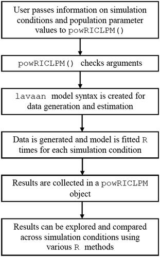
The main function powRICLPM() implements steps 2 to 5, and follows the procedure as outlined in Figure 2. First, users must specify: (a) which experimental conditions they want to explore using the sample_size, search_*, time_points, and ICC arguments, (b) the population parameter values of the lagged effects, and correlations between the within-components and between the random intercepts in the Phi, within_cor, and RI_cor arguments, respectively, and (c) their desired power level in the target_power argument. Optionally, users can specify skewness and kurtosis values to generate non-normal data, impose constraints on the estimation model, include measurement error in the simulated data, estimate measurement error variances (leading to the stable trait autoregressive trait state model) and use bounded estimation (Rosseel, 2020), which is discussed in Section 5 “Extending the Power Analysis”. Second, this input is used to compute the residual variances and covariances, and the random intercept variances for the population model. Third, for each experimental condition lavaan model syntax is generated to simulate data and estimate the RI-CLPM. Fourth, this syntax is used to repeatedly simulate data and estimate the RI-CLPM. For this, powRICLPM uses the R-package lavaan on the back-end (Rosseel 2012). Fifth, parameter estimates and standard errors are collected, and summaries are saved in an powRICLPM object. To quantify the uncertainty around the simulated power, powRICLPM implements a non-parametric bootstrapping procedure of the results: It involves taking B bootstrap samples (by default: 1000) of the significance of the parameter estimates to create a bootstrap distribution of the power for each experimental condition (Constantin et al., in press). The 95% confidence intervals of these bootstrap distributions represent the uncertainty around the simulated power. Finally, the user can use various methods such as summary(), give(), and plot() to explore the results.

Figure 2. Overview of power analysis procedure used by powRICLPM.

4.1. Illustrating Example

The illustrating example concerned determining the required sample size and number of repeated measures for detecting cross-lagged effects between self-alienation and academic amotivation with a power of 0.80. In step 2.1, it was argued that small cross-lagged effects of 0.10 and 0.15 were reasonable effect sizes to include in the power analysis (based on J. Kim et al., 2018), yet large enough to be practically interesting. Furthermore, in step 1 it was determined to include a range of proportions of between-unit variance in the experimental conditions, namely 0.3, 0.5, and 0.7. Continuing with this example, the experimental conditions to be included in the power analysis are further defined by selecting sample size candidates ranging from N = 200 to N = 2000, increasing with steps of 100, and numbers of repeated measures from T = 3 to T = 5. In total, this results in 19 sample sizes × 3 numbers of repeated measures × 3 proportions of between-unit variance, totalling 171 experimental conditions.

Following the suggestion in Section “Step 3–5: Generate data, estimate RI-CLPM, repeat”, the analysis is partitioned into a preliminary phase with reduced number of replications (R = 100), and a validation phase (R = 2000) with only those experimental conditions that are close to the desired results. The preliminary power analysis can be run using

out_preliminary <- powRICLPM(

  target_power = 0.8,

  search_lower = 200,

  search_upper = 2000,

  search_step = 100,

  time_points = c(3, 4, 5),

  ICC = c(0.3, 0.5, 0.7),

  RI_cor = 0.35,

  Phi = Phi,

  within_cor = 0.26,

  reps = 100,

  seed = 123456

)

where target_power denotes the desired power level, the search_* arguments define the lower bound, upper bound, and step size of the range of sample sizes to include, respectively, time_points denotes the numbers of time points, ICC denotes the proportions of between-person variance, RI_cor denotes the correlation between the random intercept factors, Phi refers to a matrix of lagged effects (see Appendix B), within_cor defines the correlation between the within-components, reps sets the number of Monte Carlo replications, and seed sets a seed for replicability. A visualization of the preliminary results across all 171 experimental conditions, specifically the power to detect a cross-lagged effect of 0.10 (standardized), can be obtained using

plot(out_preliminary, parameter = "wB2∼wA1")

and is displayed in Figure 3. Details about the naming conventions of parameters, ways to speed up the analysis using multicore processing, and tracking the analysis progress can be found in the package's online documentation or in the function documentation (accessible via ?powRICLPM()).

Inspecting the results using

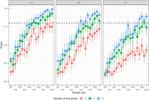
Figure 3. Results of preliminary power analysis for the RI-CLPM, based on 100 replications, for a cross-lagged effect of 0.10 (standardized). The different panels display results for conditions with a 0.3, 0.5 and 0.7 proportion of between-unit variance, respectively. The vertical error bars represent the uncertainty around the simulated power.

summary(out_preliminary)

shows that there were no fatal errors or convergence issues across any conditions in the preliminary power analysis. However, for the condition with 3 time points, 30% between person variance, and sample sizes from 200 to 500, there were 8, 5, 4, and 2 replications with inadmissible results, respectively. Investigating this further for the case with a sample size of 200, using

summary (out_preliminary, sample_size = 200, time_points = 3, ICC = 0.3)

shows that the problematic parameter is likely the variance of the random intercepts: The minimum estimate (across all replications) is negative, which leads to the inadmissible value warning. These inadmissible results might lead to bias in other parameters as well, and hence it is advisable to err on the side of caution while interpreting results for these experimental conditions (De Jonckere & Rosseel, 2022). A solution might be the use of bounded estimation, which is introduced in Section 5.

While these are only the preliminary results, the influence of sample size, number of repeated measures, and proportion of between-unit variance on power are already clearly visible in Figure 3: Experimental conditions with a higher number of repeated measures have more power to detect the cross-lagged effect of 0.10, and similarly for conditions with a relatively small proportion of stable, between-unit variance in the observed data. Focusing on the relation between number of time points and power, the preliminary results suggest that with the current range of sample sizes and proportions of between-unit variance, we cannot achieve desirable power to detect a small cross-lagged effect with 3 time points. Furthermore, the results suggest that a sample size upwards of a 1000 is required in the condition with the most advantageous proportion of between-unit variance (where proportion of between-unit variance is 0.3). For conditions with a 0.7 proportion of between-unit variance, sample sizes of approximately 1500 are needed with 5 repeated measures, whereas sample sizes upwards of 1700 are needed for 4 repeated measures. Based on these results, experimental conditions for validation are selected: The range of sample sizes is reduced to 900 to 1800, and experimental conditions with 3 repeated measures are omitted, resulting in 10 sample sizes × 2 numbers of repeated measures × 3 proportions of between-unit variance, totalling 60 experimental conditions for validation.

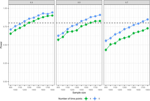
The validation results (obtained by updating the arguments of the R-code above) are displayed in Figure 4. The error bars representing the uncertainty surrounding the simulated power have shrunk considerably due to the higher number of replications, leading to more stable results. With equal proportions between- and within-unit variance (the middle panel of Figure 4, a sample size of approximately 1400 is needed for an RI-CLPM with 5 time points, and a sample size of 1600 is needed for RI-CLPM’s with 4 time points, for detecting small cross-lagged effects. Compare this to data containing higher proportions of between-unit variance, where sample sizes of 1600 or more and more than 2000 are required for RI-CLPM’s with 5 and 4 time points, respectively. In conditions with lower proportions of between-unit variance, a sample size of approximately 1100 is adequate for detecting small cross-lagged effects with 5 repeated measures, whereas a sample size of 1300 is needed for the case with 4 repeated measures.

Figure 4. Results of the validation phase of the power analysis for the RI-CLPM, based on 2000 replications. The different panels display results for conditions with a 0.3, 0.5 and 0.7 proportion of between-unit variance, respectively. The vertical error bars represent the uncertainty around the simulated power.

5. Extending the Power Analysis

So far, the primary focus has been on a basic bivariate RI-CLPM with experimental conditions varying over sample size, number of repeated measures, and proportion of between-unit variance. However, researchers might want to include additional factors in their experimental conditions to better align the power analysis to their research question or empirical context. Below various extensions that have been build into the powRICLPM package are discussed briefly, specifically: (a) imposing various constraints over time on the estimation model; (b) including measurement error in the simulated data and in the estimation model; (c) simulating non-normal data (i.e., skewness and kurtosis Blanca et al., 2013); and (d) the use of bounded estimation (Rosseel, 2020). Again, technical details on the implementation of these extensions, as well as example code, can be found in the package's online documentation and the function documentation. Extensions such as the multiple-group RI-CLPM or the multiple-indicator RI-CLPM are not supported by the package (yet), but are briefly discussed in the Discussion section. Moreover, note that the RI-CLPM is a flexible model, and that further extensions of the model are likely to be developed (e.g., Ozkok et al., 2022), each with its own idiosyncrasies when it comes to power analysis.

5.1. Constraints over Time

Means, autoregressive and cross-lagged effects, and residual variances and covariances can vary freely over time in the RI-CLPM. This is useful if the process under study is characterized by some kind of development, or if there are unequal intervals between repeated measures. For example, changes in the cross-lagged effects over time can be representative of a maturation process in individuals: The influence of one variable becomes more or less important in driving the other variable (and vice versa) as one gets older. However, imposing constraints on some of the parameters over time can be useful as well. It leads to more parsimonious results (e.g., a single set of lagged effects rather than different lagged effects between each pair of adjacent within-components), can reduce convergence issues, leads to interesting statistical equivalences with other popular panel models (for example, see Andersen, 2021; Hamaker, 2005), and increases power for the constrained parameters. In the proposed power analysis strategy above, the population model used to simulate data implicitly imposes constraints over time on the grand means μ (fixed to 0), lagged effects, and the residual variances and covariances. Essentially, the population model implies a stationary process such that for a person i the expected values $\mathbb{E}(X_{it})$ and $\mathbb{E}(Y_{it}),$ variances $\mathit{Var}(X_{it})$ and $\mathit{Var}(Y_{it}),$ and autocovariances $\mathit{Cov}(X_{it},X_{i,t+1})$ and $\mathit{Cov}(Y_{it},Y_{i,t+1})$ are independent of the time point t (Hamaker & Dolan, 2009). This was done for didactic purposes and ease of use of the power analysis strategy, as now only a a single set of population values for the lagged effects and within-component variance-covariance matrices has to be found, which can already be challenging. In contrast, the estimation model does not impose any of these constraints and freely estimates these parameters at each time point by default.

To accommodate researchers who choose to impose constraints over time on the estimation model, the powRICLPM package includes various constraint specifications via the constraints argument. It allows users to simulate the power for their specific RI-CLPM specification of interest, including a) constraints on the lagged effects over time with constraints =“lagged” b) constraints on the residual variances and covariances over time with constraints =“residuals”, or c) constraints on both the lagged effects and residual variance and covariances over time with constraints =“within”. Note that constraining the lagged effects to be time-invariant is only advized when the time interval between repeated measures is (approximately) equal (Gollob & Reichardt, 1987; Kuiper & Ryan, 2018). Furthermore, constraints on the lagged effects pertain only to the unstandardized effects, while the standardized effects are likely to be time-varying still. This is because standardization uses the variances of the within-component predictor and outcome, and these are typically not constrained to be the same over time, even with constraints on the residual variances and covariances. To obtain both time-invariant unstandardized and standardized effects, full stationarity constraints need to be imposed, which can be done with constraints =“stationarity”. These constraints are a function of the estimated autoregressive and cross-lagged effects, residual covariances, and the covariance between the within-components at the first wave. The derivations for these constraints can be found in the online supplementary materials of Mulder and Hamaker (2021).

Finally, full stationarity constraints have a long tradition in the econometric literature on dynamic panel models (for example, see Hamilton, 1994). Therefore, it is understandable that some researchers are interested in this specific specification of the RI-CLPM. However, researchers should feel comfortable with the assumptions one makes à priori when incorporating these constraints in the power analysis, as there can be various reasons why such constraints are not justified (e.g., varying time-intervals, maturation processes, development, etc.). An alternative approach is to not assume time-invariant lagged effects and residual variances beforehand (as one does if these constraints are included in the power analysis), but instead test the tenability of them using the collected data (Mulder & Hamaker, 2021).

5.2. Measurement Error

It is generally advisable to control for measurement error when analysing psychological data, as it is widely accepted that measurement error is likely to be present in psychological measurements (Savalei, 2019; Steyer et al., 1992). While the RI-CLPM actually does not include measurement error, it can in theory be added if four or more waves of data are available. This would make the model equivalent to the bivariate trait state error (TSE) model by Kenny and Zautra (1995)—later referred to as the bivariate stable trait autoregressive state trait (STARTS) model (Kenny & Zautra, 2001)—without constraints over time and with the stable trait factor loadings fixed to 1. However, the STARTS model is notorious for being empirically underidentified, commonly resulting in inadmissible solutions when sample sizes are small, leading Cole et al. (2005) to recommend a minimum of 8 waves of data (given a sample size of 500) or more. Therefore, the inclusion of measurement errors in the RI-CLPM can greatly impact the recommended sample size and number of repeated measures, not for reasons related to the power, but for reasons of empirical identification.

Within the powRICLPM package, users can include measurement error for the simulation of data (step 3) via the reliability argument, and in the estimation model (step 4) via the estimate_ME argument. The population values for the measurement error variances are determined by the package itself given the specified reliability of the indicators, the specified proportion of between-unit variance, and the within-unit component variances of 1.

5.3. Non-Normally Distributed Data

The RI-CLPM is fitted in SEM software using maximum likelihood estimation, thereby assuming multivariate normally distributed data. However, Micceri (1989) concludes that asymmetry in empirical distributions appears to be the rule for psychometric measurements rather than the exception. This is problematic as non-normality of the data can negatively impact the power of SEM models (Yuan et al., 2015). Therefore, if researchers have reason to believe that multivariate normality might not be a reasonable assumption for the data they plan on collecting, the power analysis should incorporate non-normal data as well (Yuan et al., 2015). powRICLPM allows for incorporating data with various degrees of skewness and kurtosis via the skewness and kurtosis arguments of the powRICLPM() function.

5.4. Bounded Estimation

Nonconvergence of the estimation model is disadvantageous for Monte Carlo power analyses because it reduces the effective number of replications the power analysis results are based on, and can slow down the analysis considerably as the optimization algorithm takes a long time searching for a solution that it ultimately does not find. It typically occurs when sample sizes are small (e.g., smaller than 100) and when the model is complex (e.g., when measurement error is included). Therefore, De Jonckere and Rosseel (2022) have implemented so-called bounded estimation in the R-package lavaan, placing bounds on the parameter space of the model. This prevents the optimization algorithm from searching in the completely wrong direction for parameters, for example, for negative solutions to the (residual) variances of latent variables.

Users of powRICLPM can make use of bounded estimation by setting the bounded argument to TRUE. Automatic wide bounds are then used as recommended by De Jonckere and Rosseel (2022), implying that (residual) variances (e.g., the random intercept variance, and residual variances of the within-components) have a small negative value as a lower bound, and the variances of the observed variables they load on as an upper bound. In the context of the RI-CLPM, the factor loadings are (usually) fixed, and no bounds are included for these parameters. The lagged effects are theoretically infinite, and hence there are no sensible bounds that can be placed à priori on these parameters.

6. Discussion

It is easy to underestimate the time and effort it can take to set up and execute a valid power analysis (e.g., see Footnote 2 of Paxton et al., 2001). While the increased focus within the scientific community on à prior power analysis is helpful for the progress of cumulative science, the design and execution of a valid power study is far from trivial for many applied researchers (De Jonckere & Rosseel, 2022; Maxwell et al., 2008). Nevertheless, investing time in a proper power analysis that is tailored to the particularities of one’s study is well-worth the effort, as it helps in the prevention of underpowered studies and can reduce unnecessary demand on study resources.

In this article, a 6-step Monte Carlo power analysis strategy that is tailored to the random intercept cross-lagged panel model was proposed and demonstrated. It was created with usability for applied researchers in mind and has been implemented in the R-package powRICLPM. For a basic power analysis, four sets of population parameter values are required as input, namely autoregressive and cross-lagged effects, variances and covariances for the within-unit components, the proportion of between-unit variance, and the correlation between the random intercepts. Choices for these population parameter values should be based on expert opinion or literature, or be grounded in theory. The powRICLPM package then computes the remaining population parameter values (e.g., the residual variances and covariances) and automates the process of repeatedly simulating data and estimating the model. Users can use the summary(), give(), and plot() functions to inspect the results, including convergence rates, mean square error, coverage rate, and power, among other metrics, across experimental conditions. Currently, the basic power analysis can be extended to include constraints over time on the estimation model, measurement error (i.e., the STARTS model), non-normal data, and bounded estimation.

6.1 Limitations

Step 2 of the strategy involves choosing population parameter values for the lagged effects and correlations between the within-unit components. While it is recommended to base these on theory and literature, this does not imply that any set of population parameters goes. There is a mathematical restriction on the population model-implied variance-covariance matrix that adds a degree of difficulty to the determination of these population parameter values, and introduces an element of trial-and-error to this step. Specifically, there are two restrictions that impact the population parameter values that users can specify. First, population values for the lagged effects should be chosen such that the data that are generated from these form a stable stationary system.² Second, the correlation matrix of the within-components is required to be positive definite in order to generate data from it.³ The powRICLPM package automatically checks if these restrictions are met, and throws an error otherwise. In that case, researchers should adjust the population parameter values for the lagged effects and correlations between the within-unit components accordingly, which often implies that these should be made smaller.

Furthermore, within a power analysis context one would expect the population model and the estimation model to be the same (i.e., it is assumed that the estimation model is actually the data generating model). However, as discussed in the Section “Constraints over time”, there is a discrepancy in the proposed power analysis strategy by design between the population model used to simulate the data, and the model that is estimated. The population model is based on full stationarity constraints, affecting the lagged effects, residual variances and covariances, and grand means, while the estimated model allows all parameters to be freely estimated over time. This setup was chosen for reasons of usability, without compromising the validity of the power analysis results. It ensures that users need to specify only a single set of lagged parameters and a single correlation for the within-components, which can be quite challenging already. It also implies that the power analysis results are conservative for situations where these constraints are valid, in the sense that a higher power would be achieved if constraints over time had been imposed on the estimation model. Further note that this difference between data generating mechanism and estimation model can be overruled using the constraints argument.

Moreover, it is possible that small sample sizes (<100) not only result in low statistical power, but also in bias in the parameter estimates. This is a phenomenon related to the large sample properties of maximum likelihood estimation, something that has been repeatedly reported on in the SEM literature (cf. De Jonckere & Rosseel, 2022; Rosseel, 2020; Wolf et al., 2013). The effect of small samples and a limited number of repeated measures on bias in RI-CLPM parameter estimates was not investigated here. However, it is advisable to check that bias is not a limiting factor (rather than power) for sample size recommendations when performing a power analysis using such limited sample sizes. For this, the bias as reported by powRICLPM package can be used.

A final limitation to take into account is that the sample size recommendations following the illustrating example assume a complete dataset, multivariate normally-distributed data, and no measurement error. However, missing data often do pose a problem in empirical datasets (especially in social sciences, it is nearly inevitable; Van Buuren, 2018, p. 7), observed data can show considerable deviations from normality (Blanca et al., 2013; Micceri, 1989), and many (indirect) psychological and behavioural measures are likely to include measurement error. Therefore, the conclusions from this illustrating example should be considered as lower bounds, and in practice greater sample sizes might be required to counter the negative effects of these suboptimal conditions on the power.

6.2 Comparison to Other Packages

Many different software programs have been developed for doing power analyses for SEM. They can be roughly categorized based on whether the power analysis is analytical or simulation-based, the price (free or paid option), and their generality (focusing on SEM models in general, or specific to a particular model). Below the focus is on some software packages that can be useful alternatives for RI-CLPM power analyses. For a more extensive overview of software packages available for Monte Carlo simulation studies for SEM, the reader is referred to Lee (2015).

The software package Mplus by L. K. Muthén and Muthén (2017) is a latent variable modeling program with a wide range of analysis options including Monte Carlo simulation analyses. The main advantage compared to the powRICLPM package is that it is much faster: Although no formal comparison of computation time was performed, from personal experiences a Monte Carlo power analysis for the RI-CLPM with a single experimental condition can take up to 10 minutes using powRICLPM, whereas it takes less than a minute using Mplus.⁴ Disadvantages of Mplus are that it is a paid option, does not run multiple experimental conditions simultaneously, and is not tailored to the RI-CLPM. As such, more steps need to be taken by the user to specify the power analysis for the RI-CLPM, including, for example, computing the residual variances and covariance of the within-unit components. To accommodate users of Mplus, the powRICLPM includes the powRICLPM_Mplus() function to generate Mplus syntax for RI-CLPM power analysis (for multiple experimental conditions simultaneously), which can be run subsequently in Mplus itself.

Various analytical power analysis options for SEM are available as well, including WebPower by Zhang and Liu (2018) or functions within the semTools R-package by Jorgensen et al. (2021). These options are useful, especially for the multiple group extension of the RI-CLPM (Mulder & Hamaker, 2021). The multiple group RI-CLPM is based on fitting a multiple group version of the RI-CLPM both with and without constraints across groups (e.g., the constraint of equal lagged effects), and comparing the model fit to determine whether the imposed constraints are tenable. Power thus refers to the probability of rejecting a bad-fitting model due to untenable across-group constraints in this context, rather than rejecting the null-hypothesis for a specific parameter (Wang & Rhemtulla, 2021). The effect size then refers to how much worse the constrained model fits the data compared to the more general model (with less, or no across-group constraints). Analytic solutions, like the likelihood ratio test by Satorra and Saris (1985) or power analyses based on the RMSEA by MacCallum et al. (1996), are more efficient to use for these types of power analyses than computationally intensive Monte Carlo simulation studies. For example, Jak et al. (2021) describes how the SSpower() function from the R-package semTools can be used for a multi-group SEM power analysis. It requires users to provide a SEM model without, and a model with (a single, or multiple) equality constraints across groups. The SSpower() function then performs a chi-square-based power analysis across a range of sample sizes to assess the tenability of the constraints (Jorgensen et al., 2021; Satorra & Saris, 1985).

7. Conclusion

In conclusion, this paper proposes a strategy for performing a power analysis specifically tailored to the particularities of the RI-CLPM. It is implemented in the R-package powRICLPM, which is designed to be as user-friendly as possible for applied researchers, and accommodates various extensions. Together, this paper and the R-package provide researchers with the resources to design a power analysis that produces valid recommendations for planning future research involving the RI-CLPM.

Acknowledgements

Annotated R code for the analyses performed in this article can be found in the online documentation of the powRICLPM R-package at https://jeroendmulder.github.io/powRICLPM/. I am part of the Consortium on Individual Development (CID). I would like to thank Ellen Hamaker for the discussions that have influenced this work and her useful feedback.

Disclosure statement

No potential conflict of interest was reported by the author(s).

Additional information

Funding

CID is funded through the Gravitation Program of the Dutch Ministry of Education, Culture, and Science and the Netherlands Organization for Scientific Research [NWO grant number 024.001.003].

Notes

1 To get some intuition of why increasing the number of repeated measures increases power in the RI-CLPM, it is useful to consider the concept of cluster-mean centering from the multilevel literature (Kreft et al., 1995). Rewriting Equations 1(1) $$X_{it}={\mu }_{X,t}+R{I}_{X,i}+W_{X,it},$$(1) and 2(2) $$Y_{it}={\mu }_{Y,t}+R{I}_{Y,i}+W_{Y,it}.$$(2) shows that the within-components in the model are obtained by subtracting the between-components from the observed variables. The parameters governing RI_X and RI_Y are unknown, however, and must be estimated from the data. This introduces measurement error in the between-components, and by Equations 1(1) $$X_{it}={\mu }_{X,t}+R{I}_{X,i}+W_{X,it},$$(1) and 2(2) $$Y_{it}={\mu }_{Y,t}+R{I}_{Y,i}+W_{Y,it}.$$(2) , also in the within-components (Asparouhov & Muthén, 2019). A larger number of repeated measures reduces the measurement error in RI_X and RI_Y, resulting in less error in the within-components, and thereby increasing the power to detect lagged effects (Zhang & Liu, 2018).

2 In technical terms, the eigenvalues of the matrix of lagged effects $\Phi$ should be within unit-circle.

3 In technical terms, the eigenvalues of the variance-covariance matrix of the within-unit residuals should be positive.

4 Computation time depends on many factors, including the speed of the CPU, the number of cores you are using, and the complexity of the model, etc.

Appendix A

Variance of Within-Components

The variance for the within-component of X at wave 2, $\mathit{Var}[W_{X,2}],$ can be expressed as (5) $$\begin{array}{l}Var[W_{X,2}]=Var[{\alpha }_2{W}_{X,1}+{\beta }_2{W}_{Y,1}+u_1],\hfill \\ =Var[{\alpha }_2{W}_{X,1}]+Var[{\beta }_2{W}_{Y,1}]+2{\alpha }_2{\beta }_{2}Cov[W_{X,1},W_{Y,1}]+Var[u_1],\hfill \\ ={\alpha }_2^{2}Var[W_{X,1}]+{\beta }_2^{2}Var[W_{Y,1}]+2{\alpha }_2{\beta }_{2}Cov[W_{X,1},W_{Y,1}]+Var[u_1],\hfill \\ ={\alpha }_2^2+{\beta }_2^2+2{\alpha }_2{\beta }_{2}Cov[W_{X,1},W_{Y,1}]+{\sigma }_u^2,\hfill \end{array}$$(5) which shows that it is a function of the lagged effects, ${\alpha }_2^2+{\beta }_2^2,$ the covariance between the predictors at the previous wave, $2{\alpha }_2{\beta }_{2}Cov[W_{X,1},W_{Y,1}],$ and the residual variance, ${\sigma }_u^2.$ This logic similarly applies to the variance of the within-component of academic amotivation.

Appendix B

Residual Variances and co-Variances at Wave 2 and Further

Let $\Phi$ be a square matrix of lagged effects with the diagonal elements representing autoregressive effects, and off-diagonal elements cross-lagged effects. Collecting these population parameter values for the illustrating example gives $$\Phi =\left[\begin{array}{cc}0.20& 0.15\\ 0.10& 0.30\end{array}\right].$$

Furthermore, let Σ be a variance-covariance matrix for the within-components at each time point. For the illustrating example, this results in $$\Sigma =\left[\begin{array}{cc}1& 0.26\\ 0.26& 1\end{array}\right]$$ with the diagonal elements representing the variances of the within-components, and the off-diagonal elements representing the correlation between the within-components.

C.-J. Kim and Nelson (1999, p. 27) present an expression for the unconditional covariance matrix of a stationary process as a function of the lagged effects and the residual variance covariance matrix. Rewriting this equation, the residual variances and covariances can be expressed as (6) $$\mathit{vec}(\Psi )=(I-\Phi \otimes \Phi )\mathit{vec}(\Sigma )$$(6) with $\Psi$ the residual variance-covariance matrix, I the identify matrix, and $\mathit{vec}(·)$ denoting the operation of putting the elements of a matrix into a column. Applying Equation (6)(6) $$\mathit{vec}(\Psi )=(I-\Phi \otimes \Phi )\mathit{vec}(\Sigma )$$(6) to the population parameter values of the illustrating example result in $$\Psi =\left[\begin{array}{cc}0.9219& 0.1755\\ 0.1755& 0.8844\end{array}\right]$$ where the diagonal elements represent the residual variances, and the off-diagonal represent the residual covariances needed to get within-components with a variance of 1.

References

- Andersen, H. K. (2021). Equivalent approaches to dealing with unobserved heterogeneity in cross-lagged panel models? Investigating the benefits and drawbacks of the latent curve model with structured residuals and the random intercept cross-lagged panel model. Psychological Methods, 2021, met0000285. https://doi.org/10.1037/met0000285
- Asparouhov, T., & Muthén, B. (2019). Latent variable centering of predictors and mediators in multilevel and time-series models. Structural Equation Modeling, 26, 119–142. https://doi.org/10.1080/10705511.2018.1511375
- Bandalos, D. L., & Leite, W. (2013). Use of Monte Carlo studies in structural equation modeling research. In G. R. Hancock & R. O. Mueller (Eds.), Structural equation modeling: A second course (2nd, pp. 625–666). IAP.
- Barrett, P. (2007). Structural equation modelling: Adjudging model fit. Personality and Individual Differences, 42, 815–824. https://doi.org/10.1016/j.paid.2006.09.018
- Blanca, M. J., Arnau, J., López-Montiel, D., Bono, R., & Bendayan, R. (2013). Skewness and kurtosis in real data samples. Methodology, 9, 78–84. https://doi.org/10.1027/1614-2241/a000057
- Cohen, J. (1988). Statistical Power Analysis for the Behavioral Sciences (2nd ed.). Routledge. https://doi.org/10.4324/9780203771587
- Cole, D. A., Martin, N. C., & Steiger, J. H. (2005). Empirical and conceptual problems with longitudinal trait-state models: Introducing a trait-state-occasion model. Psychological Methods, 10, 3–20. https://doi.org/10.1037/1082-989X.10.1.3.
- Constantin, M. A., Schuurman, N. K., & Vermunt, J. (in press.). A general monte carlo method for sample size analysis in the context of network models. https://doi.org/10.31234/osf.io/j5v7u
- De Jonckere, J., & Rosseel, Y. (2022). Using bounded estimation to avoid nonconvergence in small sample structural equation modeling. Structural Equation Modeling, 29, 412–427. https://doi.org/10.1080/10705511.2021.1982716
- Gische, C., & Voelkle, M. C. (2021). Beyond the mean: A flexible framework for studying causal effects using linear models. Psychometrika, 87, 868–901. https://doi.org/10.1007/s11336-021-09811-z
- Gollob, H. F., & Reichardt, C. S. (1987). Taking account of time lags in causal models. Child Development, 58, 80–92. https://doi.org/10.1111/j.1467-8624.1987.tb03492.x
- Hamaker, E. L. (2005). Conditions for the equivalence of the autoregressive latent trajectory model and a latent growth curve model with autoregressive disturbances. Sociological Methods & Research, 33, 404–416. https://doi.org/10.1177/0049124104270220
- Hamaker, E. L., & Dolan, C. V. (2009). Idiographic data analysis: Quantitative methods—From simple to advanced. In J. Valsiner, P. Molenaar, M. Lyra, & N. Chaudhary (Eds.), Dynamic process methodology in the social and developmental sciences (pp. 191–216). Springer US. https://doi.org/10.1007/978-0-387-95922-1_9
- Hamaker, E. L., Kuiper, R. M., & Grasman, R. P. (2015). A critique of the cross-lagged panel model. Psychological Methods, 20, 102–116. https://doi.org/10.1037/a0038889.
- Hamilton, J. D. (1994). Time series analysis. Princeton University Press.
- Hancock, G. R., & French, B. F. (2013). Power analysis in structural equation modeling. Structural Equation Modeling, 2013, 117–162.
- Heise, D. R. (1970). Causal inference from panel data. Sociological Methodology, 2, 3–27. https://doi.org/10.2307/270780
- Jackson, D. L. (2003). Revisiting sample size and number of parameter estimates: Some support for the N:q hypothesis. Structural Equation Modeling, 10, 128–141. https://doi.org/10.1207/S15328007SEM1001_6
- Jak, S., Jorgensen, T. D., Verdam, M. G. E., Oort, F. J., & Elffers, L. (2021). Analytical power calculations for structural equation modeling: A tutorial and Shiny app. Behavior Research Methods, 53, 1385–1406. https://doi.org/10.3758/s13428-020-01479-0.
- Jorgensen, T. D., Pornprasertmanit, S., Schoeman, A. M., & Rosseel, Y. (2021). semTools: Useful tools for structural equation modeling. https://cran.r-project.org/package=semTools
- Kenny, D. A., & Zautra, A. (1995). The trait-state-error model for multiwave data. Journal of Consulting and Clinical Psychology, 63, 52–59. https://doi.org/10.1037/0022-006X.63.1.52
- Kenny, D. A., & Zautra, A. (2001). Trait–state models for longitudinal data. New methods for the analysis of change. American Psychological Association, 2001, 243–263. https://doi.org/10.1037/10409-008
- Kim, C.-J., & Nelson, C. R. (1999). State-space models with regime Switchen. The MIT Press.
- Kim, J., Christy, A. G., Schlegel, R. J., Donnellan, M. B., & Hicks, J. A. (2018). Existential ennui: Examining the reciprocal relationship between self-alienation and academic amotivation. Social Psychological and Personality Science, 9, 853–862. https://doi.org/10.1177/1948550617727587
- Kreft, I. G., de Leeuw, J., & Aiken, L. S. (1995). The effect of different forms of centering in hierarchical linear models. Multivariate Behavioral Research, 30, 1–21. https://doi.org/10.1207/s15327906mbr3001_1
- Kuiper, R. M., & Ryan, O. (2018). Drawing conclusions from cross-lagged relationships: Re-considering the role of the time-interval. Structural Equation Modeling, 25, 809–823. https://doi.org/10.1080/10705511.2018.1431046
- Kuppens, P., Allen, N. B., & Sheeber, L. B. (2010). Emotional inertia and psychological maladjustment. Psychological Science, 21, 984–991. https://doi.org/10.1177/0956797610372634.
- Lee, S. (2015). Implementing a simulation study using multiple software packages for structural equation modeling. SAGE Open, 5, 215824401559182. https://doi.org/10.1177/2158244015591823
- Little, T. D. (2013). Longitudinal structural equation modeling. The Guilford Press.
- MacCallum, R. C., Browne, M. W., & Sugawara, H. M. (1996). Power analysis and determination of sample size for covariance structure modeling. Psychological Methods, 1, 130–149. https://doi.org/10.1037/1082-989X.1.2.130
- Maxwell, S. E., Kelley, K., & Rausch, J. R. (2008). Sample size planning for statistical power and accuracy in parameter estimation. Annual Review of Psychology, 59, 537–563. https://doi.org/10.1146/annurev.psych.59.103006.093735.
- Micceri, T. (1989). The unicorn, the normal curve, and other improbable creatures. Psychological Bulletin, 105, 156–166. https://doi.org/10.1037/0033-2909.105.1.156
- Mitchell, T. R., & James, L. R. (2001). Building better theory: Time and the specification of when things happen. The Academy of Management Review, 26, 530–547. https://doi.org/10.5465/amr.2001.5393889
- Mulder, J. D., & Hamaker, E. L. (2021). Three extensions of the random intercept cross-lagged panel model. Structural Equation Modeling, 28, 638–648. https://doi.org/10.1080/10705511.2020.1784738
- Muthén, L. K., & Muthén, B. O. (2002). How to use a Monte Carlo study to decide on sample size and determine power. Structural Equation Modeling, 9, 599–620. https://doi.org/10.1207/S15328007SEM0904_8
- Muthén, L. K., & Muthén, B. O. (2017). Mplus user’s guide. Muthén & Muthén.
- Oertzen, T., Hertzog, C., Lindenberger, U., & Ghisletta, P. (2010). The effect of multiple indicators on the power to detect inter-individual differences in change. The British Journal of Mathematical and Statistical Psychology, 63, 627–646. https://doi.org/10.1348/000711010X486633.
- Ozkok, O., Vaulont, M. J., Zyphur, M. J., Zhang, Z., Preacher, K. J., Koval, P., & Zheng, Y. (2022). Interaction effects in cross-lagged panel models: SEM with latent interactions applied to work-family conflict, job satisfaction, and gender. Organizational Research Methods, 25, 673–715. https://doi.org/10.1177/10944281211043733
- Paxton, P., Curran, P. J., Bollen, K. A., Kirby, J., & Chen, F. (2001). Monte Carlo experiments: Design and implementation. Structural Equation Modeling, 8, 287–312. https://doi.org/10.1207/S15328007SEM0802_7
- Rogosa, D. (1980). A critique of cross-lagged correlation. Psychological Bulletin, 88, 245–258. https://doi.org/10.1037/0033-2909.88.2.245
- Rosseel, Y. (2020). Small sample solutions for structural equation modeling. In R. Van de Schoot & M. Miocevic (Eds.), Small sample size solutions (pp. 226–238). Routledge.
- Satorra, A., & Saris, W. E. (1985). Power of the likelihood ratio test in covariance structure analysis. Psychometrika, 50, 83–90. https://doi.org/10.1007/BF02294150
- Savalei, V. (2019). A comparison of several approaches for controlling measurement error in small samples. Psychological Methods, 24, 352–370. https://doi.org/10.1037/met0000181.
- Steyer, R., Ferring, D., & Schmitt, M. J. (1992). States and traits in psychological assessment. European Journal of Psychological Assessment, 8, 79–98.
- Suls, J., Green, P., & Hillis, S. (1998). Emotional reactivity to everyday problems, affective inertia, and neuroticism. Personality and Social Psychology Bulletin, 24, 127–136. https://doi.org/10.1177/0146167298242002
- Usami, S. (2021). On the differences between general cross-lagged panel model and random-intercept cross-lagged panel model: Interpretation of cross-lagged parameters and model choice. Structural Equation Modeling, 28, 331–344. https://doi.org/10.1080/10705511.2020.1821690
- Van Buuren, S. (2018). Flexible imputation of missing data (2nd ed.). CRC Press.
- Wang, Y. A., & Rhemtulla, M. (2021). Power analysis for parameter estimation in structural equation modeling: A discussion and tutorial. Advances in Methods and Practices in Psychological Science, 4, 251524592091825. https://doi.org/10.1177/2515245920918253
- Winkens, B., Schouten, H. J., van Breukelen, G. J., & Berger, M. P. (2006). Optimal number of repeated measures and group sizes in clinical trials with linearly divergent treatment effects. Contemporary Clinical Trials, 27, 57–69. https://doi.org/10.1016/j.cct.2005.09.005.
- Wolf, E. J., Harrington, K. M., Clark, S. L., & Miller, M. W. (2013). Sample size requirements for structural equation models: An evaluation of power, bias, and solution propriety. Educational and Psychological Measurement, 73, 913–934. https://doi.org/10.1177/0013164413495237
- Yuan, K.-H., Tong, X., & Zhang, Z. (2015). Bias and efficiency for SEM with missing data and auxiliary variables: Two-stage robust method versus two-stage ML. Structural Equation Modeling, 22, 178–192. https://doi.org/10.1080/10705511.2014.935750
- Zhang, Z. (2014). Monte Carlo based statistical power analysis for mediation models: Methods and software. Behavior Research Methods, 46, 1184–1198. https://doi.org/10.3758/s13428-013-0424-0.
- Zhang, Z., & Liu, H. (2018). Sample size and measurement occasion planning for latent change score models through Monte Carlo Simulation. In E. Ferrer, S. M. Boker, & K. J. Grimm (Eds.), Longitudinal multivariate psychology (1st, pp. 189–211). Routledge. https://doi.org/10.4324/9781315160542-10
- Zyphur, M. J., Allison, P. D., Tay, L., Voelkle, M. C., Preacher, K. J., Zhang, Z., … Diener, E. (2020). From data to causes I: Building a general cross-lagged panel model (GCLM). Organizational Research Methods, 23, 651–687. https://doi.org/10.1177/1094428119847278
- Zyphur, M. J., Voelkle, M. C., Tay, L., Allison, P. D., Preacher, K. J., Zhang, Z., Hamaker, E. L., Shamsollahi, A., Pierides, D. C., Koval, P., & Diener, E. (2020). From data to causes II: Comparing approaches to panel data analysis. Organizational Research Methods, 109442811984728, 23, 688–716. https://doi.org/10.1177/1094428119847280