GSCA Pro—Free Stand-Alone Software for Structural Equation Modeling

Abstract

GSCA Pro is free, user-friendly software for generalized structured component analysis structural equation modeling (GSCA-SEM), which implements three statistical methods for estimating models with factors only, models with components only, and models with both factors and components. This tutorial aims to provide step-by-step illustrations of how to use the software to estimate such various models after briefly discussing model specification, estimation, and evaluation in GSCA-SEM.

Keywords:

• Generalized structured component analysis structural equation modeling
• GSCA pro
• structural equation modeling
• tutorial

1. Introduction

Researchers in various sciences are interested in investigating the path–analytic relationships between constructs such as self-esteem, depression, socioeconomic status, a region of interest, etc. As constructs themselves are abstract concepts that are not directly measurable, they are represented by proxies linked to empirical data (observed variables) in statistical models. This enables researchers to test hypotheses about the relationships between constructs (Rigdon, 2012). There are two traditional ways of statistically representing constructs: (common) factors and components (e.g., Jöreskog & Wold, 1982; Rigdon, 2012; Rigdon et al., 2017; Tenenhaus, 2008). Researchers have represented a construct as a factor, often synonymous with a latent variable or latent factor (e.g., Rhemtulla et al., 2020), under the premise that this construct is an external reality that causes observed variables to covary (e.g., Borsboom et al., 2003). On the other hand, researchers have represented a construct as a component or weighted composite of observed variables if the construct can be seen as a summary or aggregation of observed variables (e.g., Cho et al., 2022; Cho & Hwang, 2021).

When deciding on the appropriate statistical representation for a construct, it would be important to consider whether the construct is a real entity that causes or precedes observed variables, or if it is determined or preceded by those variables (e.g., Borsboom et al., 2003). If a construct is conceived to exist independently of individuals’ empirical characteristics and is the sole source of their correlations, a factor may be chosen to represent this construct in the model. Hence, observed variables manifested by factors, called reflective or effect indicators, are to be substantially intercorrelated. Factors have been used to statistically represent various psychological attributes generating observable measures in cognition, emotion, personality, and mental disorders (e.g., Borsboom et al., 2004; Guyon et al., 2018; van der Maas et al., 2014) and have served as a basis for scale construction (e.g., Bollen, 2011).

Conversely, if empirical characteristics are conceived to constitute different facets or aspects of a more general construct and compiling of the characteristics leads to this construct, a component may represent the construct in the model. For instance, body composition refers to an aggregation of body fat, muscle, and bone mineral in the body (Lohman, 1992). Physical activity is a combination of activity intensities at work, transport, and leisure, and time spent in sedentary behavior (Bull et al., 2009). Work stress may be seen as a compilation of the psychological demands of workload, workers’ perceived sense of control over their performance, safety stressors, work organization, and work atmosphere (Aittomäki et al., 2003). Socioeconomic status may be understood as a composite of an individual’s education level, income status, and prestige associated with their occupation (American Psychological Association, 2007). Observed variables generating a component in the model are referred to as composite indicators (Bollen, 2011). Different from reflective indicators, composite indicators do not have to intercorrelate as their correlations are not due to an underlying construct. Components have been utilized for index construction in various sciences (e.g., Cho & Hwang, 2023a; Fornell et al., 1996).

Structural equation modeling (SEM) has been a general statistical framework for specifying and examining how such statistical representations as factors or components are related to observed variables and how they are related among themselves, based on prior theory or knowledge. SEM has diverged into two domains, i.e., factor-based vs. component-based, depending on whether all constructs are represented as factors or components (e.g., Jöreskog & Wold, 1982; Rigdon, 2012; Rigdon et al., 2017; Tenenhaus, 2008).

The two SEM domains include different statistical methods. Covariance structure analysis (CSA; Jöreskog, 1978) has been a standard method for factor-based SEM, although there are other methods including model-implied instrumental variable methods (Bollen, 2020, 2019), factor score regression (Croon, 2002; Skrondal & Laake, 2001), structured factor analysis (Cho & Hwang, 2023b), and generalized structured component analysis with measurement errors incorporated (GSCA_M; Hwang et al., 2017). On the other hand, generalized structured component analysis (GSCA; Hwang & Takane, 2004, 2014) is the most general method for component-based SEM, which can include a long-standing component-based method, partial least squares path modeling or PLS-SEM, as a special case (Cho et al., 2022; Hwang & Cho, 2020). It has been theoretically and empirically shown that when an SEM method developed for one domain is used for the other domain, it results in biased solutions (Hwang et al., 2021; Sarstedt et al., 2016). For example, CSA will provide biased estimates of parameters in models with components (e.g., component loadings and path coefficients relating components), whereas GSCA will yield biased estimates of parameters in models with factors (e.g., factor loadings and path coefficients connecting factors).

Over the decades, all the methods have been used exclusively for either of the two SEM domains, permitting researchers to estimate models with either factors or components only. However, in practice, it does not seem uncommon that researchers may need to include both factors and components in the model to simultaneously consider a broad array of constructs from different disciplines. For example, researchers can be interested in examining how physical activity and body composition, both of which may be represented by components, affect the risk and severity of depressive disorders, which may be represented by factors (von Zimmermann et al., 2020).

Only recently, the next generation of SEM methods has emerged that permits estimating models with both factors and components in a unified framework. It includes consistent partial least squares (PLSc; Dijkstra, 2011; Dijkstra & Henseler, 2015a, 2015b) and integrated generalized structured component analysis (IGSCA; Hwang et al., 2021). As compared to PLSc, IGSCA can estimate more complex models, e.g., those with cross loadings, and is less prone to the occurrence of improper solutions. In addition, a recent study shows that IGSCA generally tends to perform better than PLSc under various situations (Hwang et al., 2021).

GSCA Pro is a stand-alone software program that implements GSCA, GSCA_M, and IGSCA for estimating structural equation models with factors only, models with components only, or models with both factors and components, respectively. The collection of the three methods is termed GSCA-SEM (Hwang, Cho, et al., 2023). The software is free of charge and can be downloaded from its website (www.gscapro.com). It provides a graphical user interface that allows users to easily draw their model as a path diagram, fit GSCA-SEM to the model, and obtain results.

In this tutorial, we aim to introduce GSCA Pro to researchers and practitioners as free and user-friendly software for GSCA-SEM. We begin by presenting an account of the three methods in GSCA-SEM, focusing on model specification, estimation, and evaluation. We then provide step-by-step illustrations of using the software to apply GSCA-SEM’s methods for estimating models with factors only, with components only, and with both factors and components.

2. Brief Introduction to GSCA-SEM

2.1. Model Specification and Estimation

As stated earlier, GSCA Pro is software for GSCA-SEM, an umbrella term that includes three SEM methods—GSCA, GSCA_M, and IGSCA. In model specification, GSCA involves three sub-models: the weighted relation, (component) measurement, and structural models. The weighted relation model explicitly defines a component as a weighted sum of indicators, where the weights assigned to a set of indicators to form a component are parameters. The (component) measurement model is used to specify the regression relationships of a set of indicators on its component, in which the regression coefficients called component loadings constitute parameters. The structural model is to specify the path analytic relationships between components, consisting of the (component) path coefficients as parameters. Specifically, the three sub-models are given as follows. (1) $$\mathbf{\gamma }=\mathbf{Wz} \left(\text{weighted relation model}\right)$$(1) (2) $$\mathbf{z}=\mathbf{C}\mathbf{\gamma }+\mathbf{\epsilon } \left(\text{measurement model}\right)$$(2) (3) $$\mathbf{\gamma }=\mathbf{B}\mathbf{\gamma }+\mathbf{\zeta } \left(\text{structural model}\right),$$(3) where z is a J by 1 vector of indicators, γ is a P by 1 vector of components, W is a P by J matrix of weights, C is a J by P matrix of component loadings, B is a P by P matrix of (component) path coefficients, and ε and ζ are J by 1 and P by 1 vectors of errors in the measurement and structural models, respectively.

The three sub-models are combined into a single equation, referred to as the GSCA model, as follows. (4) $$\begin{array}{l}\left[\begin{array}{c}z\\ \gamma \end{array}\right]=\left[\begin{array}{c}C\\ B\end{array}\right]\gamma +\left[\begin{array}{c}\epsilon \\ \zeta \end{array}\right]\\ \left[\begin{array}{c}z\\ Wz\end{array}\right]=\left[\begin{array}{c}C\\ B\end{array}\right]Wz+\left[\begin{array}{c}\epsilon \\ \zeta \end{array}\right]\\ \left[\begin{array}{c}I\\ W\end{array}\right]z=\left[\begin{array}{c}C\\ B\end{array}\right]Wz+\left[\begin{array}{c}\epsilon \\ \zeta \end{array}\right]\\ Vz=AWz+e,\end{array}$$(4) where I is the identity matrix of order J, V =$\left[\begin{array}{c}I\\ W\end{array}\right],$ A =$\left[\begin{array}{c}C\\ B\end{array}\right],$ and e =$\left[\begin{array}{c}\mathbf{\epsilon }\\ \mathbf{\zeta }\end{array}\right]$ (Hwang & Takane, 2014, p. 19). In its general form, the GSCA model can be considered a component-generating model, where a component is obtained by aggregating a set of given indicators in such a way that the component is to explain the total variance of its indicators and other components (Cho et al., 2022).

On the other hand, when applying GSCA_M for estimating models with factors only, researchers can specify the (reflective) measurement and structural models as in typical factor-based SEM. The (reflective) measurement model is used to specify the regression relationships of a set of indicators on its factor, containing factor loadings as parameters. The structural model is to specify the path-analytic relationships between factors, in which the (factor) path coefficients are parameters. The two sub-models can be combined into a single formulation, such as the LISREL (Jöreskog, 1973), Bentler–Weeks (Bentler & Weeks, 1980) or reticular action (McArdle & McDonald, 1984) model.

Lastly, IGSCA, which is used for estimating models with both factors and components, involves the sub-models for GSCA and GSCA_M. This indicates that IGSCA includes all the parameters in GSCA and GSCA_M as its parameters, including weights, factor and component loadings, and path coefficients connecting factors and/or components.

All the methods in GSCA-SEM typically assume that indicators and components/factors are standardized to have zero means and unit variances. They seek to minimize a single least squares optimization function via an iterative algorithm to estimate all model parameters simultaneously (Hwang et al., 2017, 2021; Hwang & Takane, 2004), although other estimation procedures have been proposed (e.g., Choi & Hwang, 2020). This least squares estimation does not resort to any distributional assumption, such as multivariate normality of indicators. The methods estimate the standard errors and confidence intervals of their parameter estimates based on the non-parametric (percentile) bootstrap method (Davison & Hinkley, 1997; Efron, 1979; Jung et al., 2019).

As stated above, GSCA is based on its own population model (i.e., the GSCA model) and can serve as an unbiased estimator for the GSCA model (Cho et al., 2022) and other models with components (e.g., Cho & Choi, 2020; Dijkstra, 2013, 2017). On the other hand, it seems more reasonable to regard GSCA_M and IGSCA simply as an unbiased estimator for models with factors only and models with factors and components, respectively. While estimating model parameters, these methods additionally estimate factor scores as weighted sum scores of indicators with their uniqueness terms removed (Hwang et al., 2017, 2021). This procedure of estimating both factor scores and other model parameters helps avoid the occurrence of improper solutions (Cho & Hwang, 2023b; Hwang et al., 2017).

2.2. Model Evaluation

2.2.1. Overall and Local Model Fit Measures

GSCA Pro provides several measures to evaluate the model’s overall fit. There are different types of overall model fit measures for the three methods of GSCA-SEM. We begin by describing model fit measures commonly used in the three methods. Specifically, the software offers two absolute fit measures, GFI and SRMR, both of which are proportional to the difference between the sample and model-implied covariance matrices. There are rule-of-thumb cutoff values for these measures, which may be indicative of an acceptable level of fit under models with factors only (Hu & Bentler, 1999), those with components only (Cho et al., 2020), and those with both factors and components (Cho et al., 2022). Table 1 presents these recommendations. Note that in GSCA-SEM, errors within a block of indicators per component in the measurement model are intercorrelated, ensuring that the model can fully account for the within-block sample covariances of the indicators (Cho & Choi, 2020; Cho et al., 2022). As a result, any discrepancies between the sample and implied covariance matrices of indicators for components are confined to the covariances of indicators across different blocks, determining the GFI and SRMR values in GSCA-SEM.

Table 1. Rule-of-thumb guidelines for model evaluation in GSCA-SEM.

Criterion		Rules of thumb	References
Overall model fit	Models with factors only (GSCAM)	GFI ≥ 0.95 and SRMR ≤ 0.08	Hu and Bentler (1999)
	Models with components only (GSCA)	When N = 100, GFI ≥ 0.89 and SRMR ≤ 0.09. SRMR ≤ 0.09 may be prioritized over GFI ≥ 0.89. If SRMR ≤ 0.09, GFI ≥ 0.85 may still be indicative of an acceptable fit When N > 100, GFI ≥ 0.93 or SRMR ≤ 0.08 OPE < 1	Cho et al. (2020) Cho et al. (2019)
	Models with both factors and components (IGSCA)	When N = 100, GFI ≥ 0.88 and SRMR ≤ 0.10 When N = 200, GFI ≥ 0.91 and SRMR ≤ 0.08. SRMR ≤ 0.08 may be prioritized over GFI ≥ 0.91 When N > 500, GFI ≥ 0.95 or SRMR ≤ 0.06	Cho et al. (2022)
Measurement model with factors	Internal consistency reliability	Cronbach’s α ≥ 0.7, but ≤ 0.95 ρC ≥ 0.7, but ≤ 0.95	Cronbach and Meehl (1955), Diamantopoulos et al. (2012), Drolet and Morrison (2001), and Jöreskog (1971)
	Convergent validity	AVE ≥ 0.50	Götz et al. (2010)
	Discriminant validity	For conceptually similar factors, HTMT < 0.90 For conceptually different factors, HTMT < 0.85	Henseler et al. (2015), and Franke & Sarstedt (2019)
	Factor loadings’ statistical significance and relevance	A factor loading estimate is statistically significant if its 95% percentile confidence interval does not contain zero A large loading estimate (in absolute value) indicates a stronger correlation with the corresponding factor
Measurement model with components	Local model fit	OPEM < 1	Cho et al. (2019)
	Unidimensionality	Kaiser criterion PVE: A single component explains at least 70% of the indicators’ variance	Kaiser (1960), and Jolliffe and Cadima (2016)
	Component weights’ statistical significance and relevance	A component weight estimate is statistically significant if its 95 percentile confidence interval does not include zero The larger the weight estimate (in absolute value), the stronger the indicator’s relevance for forming the respective component	Hwang and Takane (2014) and Hwang et al. (2023)
	Component loadings’ statistical significance and relevance	A component loading estimate is statistically significant if its 95% percentile confidence interval does not contain zero A large loading estimate (in absolute value) indicates a stronger correlation with the corresponding component	Hwang and Takane (2014) and Hwang et al. (2023)
Structural model with factors and/or components	Local model fit	OPES < 1 (structural model with components only)	Cho et al. (2019)
	Collinearity	Critical level of collinearity when VIF ≥ 5 Potential collinearity when VIF between 3 and 5 Ideally, VIF < 3	Chatterjee and Price (1977), Hair et al. (2011), Hair et al. (2019), and Hwang et al. (2023)
	Path coefficients’ statistical significance and relevance	A path coefficient estimate is statistically significant if its 95% percentile confidence interval does not contain zero The larger the path coefficient estimate, the stronger the effect. Consider the f^2 as an effect size measure. f^2 = 0.02, 0.15, and 0.35 may be interpreted as small, medium, and large effect sizes, respectively, as benchmarks	Cohen (1988) and Hwang et al. (2023)
	Explanatory power	R^2 values should always be interpreted in the context of the model R^2 ≥ 0.90 of constructs measuring perceptions, attitudes, or intentions indicate potential overfit.	Sharma et al. (2019) and Hwang et al. (2023)

The software provides another absolute fit measure, FIT, which indicates how much variance of both indicators and factors/components is explained by the model, ranging from 0 to 1. This measure is comparable to the R squared in linear regression, and there is no rule-of-thumb cutoff for the FIT, which may be indicative of an acceptable level of fit. Moreover, GSCA Pro provides two local model fit measures for the three GSCA-SEM methods. The FIT_M indicates how much variance of indicators is explained by a given measurement model, whereas the FIT_S indicates how much variance of factors and/or components is accounted for by a given structural model. Similar to the FIT, both local absolute fit measures range from 0 to 1, for which no rule-of-thumb cutoff values indicative of an acceptable level of fit exist.

GSCA Pro reports the above overall and local fit measures for all GSCA-SEM methods. Furthermore, when researchers apply GSCA to estimate a model with components only, the software provides a few additional measures for overall or local model fit. They include AFIT (adjusted FIT) and OPE (out-of-sample prediction error) as overall model fit measures and OPE_M and OPE_S as local model fit measures. The AFIT (Hwang et al., 2007) is comparable to the adjusted R squared in linear regression, which takes model complexity into account. This comparative fit measure should be used only for comparing models in their explanatory powers. The model that maximizes the AFIT may be chosen over the other models. The OPE shows the prediction error of a given model (Cho et al., 2019). Whereas the other overall fit measures focus on the total variance explained in the sample at hand (i.e., an in-sample) or the differences between model-implied and in-sample covariances, the OPE indicates how the model predicts a sample of unseen observations (i.e., an out-of-sample) as compared to a null model that predicts the out-of-sample using the in-sample means of dependent variables. An OPE value less than 1 indicates that the model has a smaller out-of-sample prediction error than the null model on average. This is also a comparative fit measure, which can be used only to compare different models’ prediction errors. The OPE_M and OPE_S represent the average out-of-sample prediction errors of the measurement and structural models against their null models, where the in-sample means of indicators or components are used to predict an out-of-sample. An OPE_M or OPE_S value below 1 denotes that the respective sub-model leads to a smaller out-of-sample predictor error than the null model on average. Like the OPE, these local measures can be used only for comparing the prediction errors of different measurement or structural models. Note that the OPE, OPE_M, and OPE_S are calculated based on the bootstrap method. To obtain more reliable values of these indices, it is recommended to apply a large number of bootstrap samples, for example, 2000 samples (Cho et al., 2019).

2.2.2. Measurement Model Evaluation

GSCA Pro provides various metrics to assess the measurement model in GSCA-SEM. If the measurement model contains factors only (i.e., the reflective measurement model) and is estimated by GSCA_M, it provides reliability and validity criteria that have been well-known in the factor-based SEM literature (e.g., Bollen, 1989; Kline, 2016). For example, the software provides metrics for measuring internal consistency reliability, including Cronbach’s α (Cronbach, 1951; Cronbach & Meehl, 1955) and Dillon–Goldstein’s rho (Chin, 1998) or Jöreskog’s (1971) composite reliability ρ_C. Unlike Cronbach’s α, ρ_C does not assume equal population loadings (i.e., tau-equivalence). Moreover, the software provides the average variance extracted (AVE), the average value of all squared factor loadings, to examine the proportion of variance that a factor explains in its reflective indicators as a way of checking convergent validity. It also reports the heterotrait–monotrait (HTMT) ratio per pair of factors (Henseler et al., 2015), which assesses the extent to which a factor is empirically distinct from other factors, as a way of examining discriminant validity. A large HTMT value between the pair of factors suggests that the correlations of reflective indicators across the two factors are higher than those of reflective indicators within each factor, implying a low level of discriminant validity. Note that Rönkkö and Cho (2022) show that the HTMT ratio is a disattenuated correlation using parallel reliability or the standardized alpha, which is based on the parallel assumption that the variances of reflective indicators per factor are the same and their covariances are the same. It seems difficult to satisfy the parallel assumption in practice (McNeish, 2018).¹

Furthermore, the software gives the bootstrap standard errors and 95% bootstrap confidence intervals (CI) of factor loading estimates to examine the statistical significance of the estimates. Using the bootstrap CI rather than a t-test (calculated by dividing the parameter estimate by its bootstrap standard error) is recommended because the t-test is parametric, assuming the normality assumption. Although there are several approaches for estimating bootstrap CIs, the software provides the percentile bootstrap CI as it seems to perform best in terms of coverage and balance (Jung et al., 2019). Also importantly, the factor loading estimates of reflective indicators should be large in magnitude, indicating the indicators’ substantive relevance to their factors (e.g., MacCallum et al., 1999, 2001).

When the measurement model contains components only (i.e., the component measurement model) and is estimated by GSCA, the software provides different metrics to evaluate this sub-model as it becomes irrelevant to check the internal consistency and validity of factors underpinning reflective indicators (Bollen, 1989). For example, it provides the bootstrap standard errors and 95% bootstrap CIs of the estimates of both component weights and loadings. By checking the statistical significance of the weight estimates per component, we may evaluate whether a composite indicator makes a statistically significant contribution to forming a component. If the model is unidimensional, composite indicators’ weights per component are proportional to their loadings, which are easier to interpret as correlations (Dijkstra, 2017). Under the unidimensional model, we may thus focus on looking into the statistical significance of the component loading estimates and their substantive relevance. Moreover, the software provides the proportion of variance explained (PVE), which shows how much the total variance of a set of composite indicators is explained by its corresponding component on average, as in principal components analysis. If a single component explains 70% or higher of the total variance of a set of composite indicators, this may be indicative of unidimensionality for the block (Jolliffe & Cadima, 2016). Another way of checking unidimensionality is to apply an eigenvalue decomposition to a set of composite indicators. According to the Kaiser criterion (Kaiser, 1960), if only the largest eigenvalue is greater than one, this may be indicative of unidimensionality per set of indicators.

When the measurement model consists of both factors and components and is estimated via IGSCA, the software provides all the metrics for the measurement model with factors or components. Researchers can use them to evaluate factor-based and component-based parts of the measurement model, as discussed above. Table 1 also presents rule-of-thumb recommendations for the metrics for assessing the measurement model.

2.2.3. Structural Model Evaluation

GSCA Pro provides different metrics that can be used for evaluating the structural model. Unlike the case of measurement model assessment, researchers can use these metrics regardless of whether the structural model includes factors or components, or both. The software offers the variance inflation factor (VIF; Chatterjee & Price, 1977) values for independent factors/components per dependent factor/component for checking potential multicollinearity, which can lead to less reliable path coefficient estimates or unexpected sign changes (Hwang & Takane, 2014, Chapter 8). The software also provides the estimates of path coefficients connecting factors and/or components, along with their bootstrap standard errors and percentile CIs, which can be used to evaluate the path coefficients’ relevance and their statistical significance. In addition, GSCA Pro gives the coefficient of determination (R²) and an effect size measure such as f² for each dependent factor/component. Table 1 also summarizes all the metrics and their benchmark values for assessing the structural model.

3. Illustrations

We demonstrate the application of GSCA Pro to three examples that consider the estimation of 1) a model with components only via GSCA, 2) a model with factors only via GSCA_M, and 3) a model with both factors and components via IGSCA. We concentrate on a basic single-group analysis in each example. We begin by describing how to prepare a dataset for the software in general.

3.1. Data Preparation for GSCA Pro

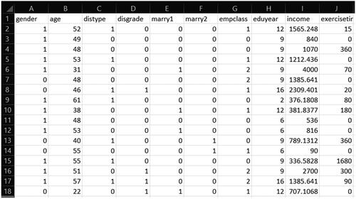
When preparing a dataset for GSCA Pro, we include the names of indicators in the first row of the dataset. If the first row does not contain the names of indicators, the indicators will be automatically labeled V₁, V₂, …, and V_J, where J is the number of indicators. The following rows include the individual scores of N observations on the indicators, where each row represents the scores of a single observation per indicator. These data should be numeric only. All missing values are by default denoted by −9999. We can also assign different numeric values to denote missing values. The software can import the data in .txt, .csv, and .xlsx file formats. Figure 1 displays part of Jun et al. (2011)’s data for GSCA Pro, which we use in the next section.

Figure 1. Part of Jun et al. (2011)’s data uploaded in GSCA Pro.

GSCA Pro currently does not support multi-core parallel processing. While there is no preset RAM requirement for the software, the amount of memory needed will depend on the sizes of the datasets and models in question. It is worth noting that although GSCA Pro takes in an N by J data matrix, it transforms this matrix into the J by J covariance matrix of indicators, which is subsequently utilized to estimate parameters (Hwang & Takane, 2014, p. 74). This procedure can significantly reduce the computational burden, particularly with large sample sizes.

3.2. Application of GSCA for Estimating a Model with Components Only

We illustrate the use of GSCA Pro to apply GSCA to estimate a model with components only. The example data and model come from Jun et al. (2011), which examine the relationships among four constructs: socioeconomic status (SES), health behavior, health status, and job satisfaction of workers with disabilities in South Korea. As part of a panel survey on the employment of workers with disabilities conducted in 2008, the data include 1,212 wage workers with disabilities (N = 1212).

As exhibited in Table 2, there are 15 indicators for SES, health status, and job satisfaction, whereas there is a single indicator for health behavior. Also, there are six covariates, including gender, age, level of disability, type of disability, and two dummy variables of marital status labeled marital status 1 and marital status 2. We contemplate that SES, health status, and job satisfaction can be represented as components rather than factors because their indicators seem to characterize distinct aspects of the constructs, which may add up to produce the constructs. The data and GSCA Pro project file are available at www.gscapro.com/examples.

Table 2. Constructs and items/indicators in Jun et al. (2011).

Construct	Items	Indicator name
SES Health behavior Health status Job satisfaction	Type of employment Number of years of education Income Daily hours of exercise (in minutes) Subjective health status (1 = very bad, 4 = very good) Satisfaction with health (1 = very dissatisfied, 5 = very satisfied) Number of chronic diseases Satisfaction with (1 = very dissatisfied, 5 = very satisfied) Salary Job security Job duties and responsibilities Work environments Hours of work Career development opportunities Interpersonal communication/relationships Fairness in performance appraisals Employee benefits	ses1 ses2 ses3 hb hs1 hs2 hs3 js1 js2 js3 js4 js5 js6 js7 js8 js9

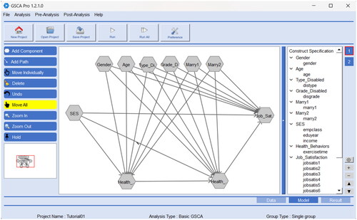
To apply GSCA to this example, we begin by selecting Analysis → GSCA→ Basic GSCA → single group in the GSCA Pro menu. Then, we specify the structural model as follows. We click on the icon Add Component, move the cursor to a position in the main modeling window where we want to place a component and click as many times as the number of components. Note that GSCA Pro requires specifying a covariate as a single-indicator component as well, to which the covariate itself is assigned as the indicator. Thus, in the example, we should also include health behavior and the six covariates as components and have a total of 10 components, of which three are multiple-indicator components (i.e., SES, health status, and job satisfaction) and the others are single-indicator components. Thus, ten clicks create the components. GSCA Pro will display the new components as a hexagon, which are by default labeled new1 to new10. We then specify a path coefficient between the components as follows. We click on the icon Add Path and drag an arrow from each independent component to its dependent component. Repeat this process to specify the remaining path coefficients.

Next, we specify the measurement model as follows. We double-click on each component (or hexagon) to open the Assign Indicators to Constructs window, which displays all available indicators in the dataset in the left-hand box. We select the indicators that we want to assign to the component and move them to the (empty) right-hand box (e.g., the indicators js1 to js9 for Job Satisfaction). The label “Free” next to each indicator means that its loading is a free parameter to be estimated. We repeat the same procedure for the remaining components. In this way, we can complete all model specification in GSCA Pro. Figure 2 displays the completed model specification for the example in GSCA Pro. The software exhibits which component is linked to which indicators in the measurement model on the right-hand panel, as well as the path diagram of the structural model on the main window.

Figure 2. An illustration of applying GSCA in GSCA Pro.

Once the model specification is complete, we estimate the model via GSCA by clicking on the Run icon in the menu bar. When the GSCA algorithm has converged, basic analysis results are automatically displayed in the Result tab. The top of the tab shows an estimation summary with details regarding, for example, analysis type (e.g., “Basic GSCA/single group” in our example), the number of bootstrap samples, and the algorithm’s convergence (i.e., the number of iterations and convergence criterion).

We follow the guidelines in Table 1 to assess the estimated model and interpret the results. The model shows GFI = .98, SRMR = .04, FIT = .50, AFIT = .50, and OPE = .50. Given the sample size, both GFI and SRMR values suggest an acceptable model fit. Also, the model explains about 50% of the total variance of all the indicators and components. Moreover, it has a smaller average prediction error than the null model. As discussed, the AFIT and OPE are comparative fit indices for model comparison from the explanation and prediction perspectives, respectively. Furthermore, the model shows FIT_M = .71 and FIT_S = .04, indicating that the measurement model explains 71% of the variance of all indicators, whereas the structural model explains 4% of the variance of the components. The model also shows OPE_M = .29 and OPE_S = .96, denoting that both measurement and structural models lead to smaller average prediction errors than their null models. The OPE_M and OPE_S can be used for comparing different specifications of the sub-models from the prediction perspectives.

Table 3 presents the estimates of the component weights and loadings, along with their bootstrap standard errors and 95% percentile CIs. Both weight and loading estimates for the single-indicator components are one, indicating that these components are the same as their respective indicator. The weight estimates per multiple-indicator component are statistically significant (i.e., none of their 95 CIs contains zero). They do not vary substantially, indicating that the indicators contribute similarly to forming the corresponding component. All component loading estimates for the multiple-indicator component are also statistically significant and generally large, suggesting that the components are highly related to their corresponding indicators.

Table 3. GSCA’s estimates of weights and loadings in the measurement model.

Component	Indicator	Weights			Loadings
		Estimate	SE	95% CI	Estimate	SE	95% CI
SES	ses1 ses2 ses3	0.50 0.40 0.45	0.01 0.01 0.01	[0.48, 0.53] [0.37, 0.42] [0.42, 0.47]	0.79 0.70 0.73	0.01 0.02 0.02	[0.76, 0.81] [0.65, 0.73] [0.70, 0.76]
Heath behavior	hb	1	0	0	1	0	0
Heath status	hs1 hs2 hs3	0.46 0.46 -0.31	0.01 0.01 0.01	[0.43, 0.48] [0.44, 0.48] [-0.33, −0.29]	0.88 0.89 -0.61	0.01 0.01 0.02	[0.86, 0.89] [0.88, 0.91] [-0.65, −0.56]
Job satisfaction	js1 js2 js3 js4 js5 js6 js7 js8 js9	0.14 0.17 0.17 0.16 0.14 0.16 0.13 0.13 0.16	0.00 0.00 0.01 0.01 0.00 0.00 0.00 0.00 0.00	[0.13, 0.15] [0.16, 0.18] [0.15, 0.18] [0.15, 0.17] [0.13, 0.15] [0.15, 0.17] [0.12, 0.14] [0.12, 0.14] [0.15, 0.17]	0.71 0.76 0.84 0.83 0.70 0.76 0.63 0.71 0.72	0.02 0.01 0.01 0.01 0.02 0.02 0.02 0.02 0.02	[0.68, 0.74] [0.73, 0.79] [0.83, 0.86] [0.81, 0.85] [0.67, 0.74] [0.73, 0.79] [0.59, 0.67] [0.67, 0.74] [0.69, 0.75]

Table 4 provides the estimates of the path coefficients connecting the components and their bootstrap standard errors and 95% percentile CIs. Focusing on the relationships among the components of main interest, we find that SES has positive and statistically significant effects on health behavior (0.08, SE = 0.04, 95% CI = [0.01, 0.15]), health status (0.20, SE = 0.03, 95% CI = [0.15, 0.26]), and job satisfaction (0.44, SE = 0.03, 95% CI = [0.39, 0.49]). Also, health behavior has a positive and statistically significant impact on health status (0.05, SE = 0.02, 95% CI = [0.01, 0.10]), which has a positive and statistically significant influence on job satisfaction (0.21, SE = 0.03, 95% CI = [0.15, 0.26]).

Table 4. GSCA’s estimates of path coefficients in the structural model. IV = independent variable and DV = dependent variable.

IV	DV	Estimate	SE	95% CI
Gender	Health behavior	0.08	0.02	[0.02, 0.12]
	Health status	0.11	0.03	[0.06, 0.16]
	Job satisfaction	−0.13	0.03	[-0.18, −0.08]
Age	Health behavior	0.09	0.03	[0.03, 0.16]
	Health status	−0.24	0.03	[-0.30, −0.17]
	Job satisfaction	0.07	0.03	[0.01, 0.14]
Type of disability	Health behavior	0.03	0.03	[-0.03, 0.10]
	Health status	0.06	0.03	[0.00. 0.12]
	Job satisfaction	−0.04	0.03	[-0.09, 0.01]
Level of disability	Health behavior	0.04	0.03	[-0.03, 0.11]
	Health status	0.02	0.03	[-0.04, 0.08]
	Job satisfaction	0.07	0.03	[0.02, 0.12]
Marital status1	Health behavior	0.00	0.04	[-0.07, 0.08]
	Health status	−0.01	0.03	[-0.07, 0.06]
	Job satisfaction	−0.03	0.03	[-0.10, 0.04]
Marital status2	Health behavior	0.01	0.03	[-0.05, 0.08]
	Health status	−0.07	0.03	[-0.14, −0.01]
	Job satisfaction	0.02	0.03	[-0.03, 0.08]
SES	Health behavior	0.08	0.04	[0.01, 0.15]
	Health status	0.20	0.03	[0.15, 0.26]
	Job satisfaction	0.44	0.03	[0.39, 0.49]
Health behavior	Health status	0.05	0.02	[0.01, 0.10]
Health status	Job satisfaction	0.21	0.03	[0.15, 0.26]

When we click on the View Full Result button on the left-hand side in the Result tab, GSCA Pro provides additional information to evaluate the measurement and structural models, as displayed in Table 5. For example, in the Construct Quality Measures table, the software shows each multiple-indicator component’s dimensionality, which indicates the number of components extracted from the set of composite indicators with an eigenvalue greater than one. The dimensionality of SES, health behavior, and job satisfaction turns out to be one. The PVE values of these components range from 0.55 to 0.65. Moreover, the software provides the VIF values of all independent components and covariates for each dependent component in the structural model. Age has the largest VIF value of 1.65 for job satisfaction. This VIF is below the rule-of-thumb cutoffs in Table 1, indicating that multicollinearity is of little concern in the example. In addition, the software provides the R² values for all dependent components, which reflect the explanatory power (in-sample error) of the structural model for the dependent components. It also reports the f² value of each independent variable per dependent component, which can be interpreted as described in Table 1. We can also export the entire report as a .csv file by using the Export Result option at the top-left of the tab.

Table 5. Additional metrics for model assessment in the GSCA example.

	Dimensionality	PVE	R^2
SES	1	0.55
Health behavior	1	1	0.02
Health status	na	0.65	0.17
Job satisfaction	1	0.55	0.26
		VIF	Effect size (f^2)
Gender	Health behavior	1.15	0.01
	Health status	1.16	0.01
	Job satisfaction	1.17	0.02
Age	Health behavior	1.58	0.01
	Health status	1.59	0.06
	Job satisfaction	1.65	0.01
Type of disability	Health behavior	1.07	0.00
	Health status	1.07	0.00
	Job satisfaction	1.07	0.00
Level of disability	Health behavior	1.09	0.00
	Health status	1.10	0.00
	Job satisfaction	1.09	0.00
Marital status1	Health behavior	1.52	0
	Health status	1.52	0
	Job satisfaction	1.52	0.00
Marital status2	Health behavior	1.20	0
	Health status	1.20	0.01
	Job satisfaction	1.20	0
SES	Health behavior	1.18	0.01
	Health status	1.18	0.04
	Job satisfaction	1.23	0.24
Health behavior	Health status	1.02	0.00
Health status	Job satisfaction	1.20	0.04

na: not applicable.

3.3. Application of GSCA_M for Estimating a Model with Factors Only

We demonstrate how to use GSCA Pro to apply GSCA_M to estimate a model with factors only. The example data and model come from Boubker and Douayri (2020), which investigate the relationships among consumer satisfaction (CS), brand attitude (BA), brand preference (BP), and purchase intention (PI) in Morocco. The data include 195 Moroccan consumers of dairy products (N = 195). As shown in Table 6, there are 16 indicators for the four constructs. We posit that all the constructs may be represented as factors, as such psychological attributes reflecting individuals’ feelings, beliefs, or preferences have been proxied by factors (e.g., Borsboom et al., 2004; Guyon et al., 2018) and the indicators for each construct appear similar, whose correlations may be derived by their underlying construct, rather than they determine the construct. The data and GSCA Pro project file are available at www.gscapro.com/examples.

Table 6. Constructs and items/indicators in Boubker and Douayri (2020).

Construct	Items	Indicator name
	Indicate your level of agreement with the following statements: (1 = total disagreement, 5 = total agreement)
Consumer satisfaction Brand attitude Brand preference Purchase intentions	I am satisfied with my decision to customize the product from this brand. Consuming dairy products from this brand is a good idea. I am happy that I customized the product from this brand. Consuming dairy products of this brand is a good choice. I am disappointed with this brand (reverse scoring). Unpleasant/ pleasant Bad/ good differential scale Unfavorable/favorable I like this brand better than any other brand of dairy products. I would consume this brand more than any other brand of dairy products. I would be inclined to buy dairy products from this brand over rather than from other brands. This is my preferred brand overall brands of dairy products. What is the likelihood that you would recommend this brand to someone close to you? (1 = low, 5 = high) You were again consuming dairy products offered by this brand? Would you recommend dairy products offered by this brand to a friend and/or relative? Were you buying products offered by this brand?	cs1 cs2 cs3 cs4 cs5 ba1 ba2 ba3 bp1 bp2 b43 ba4 pi1 pi2 pi3 pi4

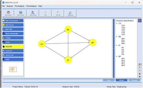
To apply GSCA_M to the example, we begin by selecting Analysis → GSCAm → Basic GSCAm → single group in the GSCA Pro menu. Then, we similarly specify the structural model as described in the previous section. We click on the icon Add Factor and click as many times as the number of factors in the main modeling window. In our example, four clicks create the factors, displayed as a circle and initially labeled new1 to new4. We then specify a path coefficient between the factors by clicking on the icon Add Path and dragging an arrow from an independent factor to its dependent factor. We also specify the measurement model as described in the previous section, by opening the Assign Indicators to Constructs window for each factor (or circle). Figure 3 displays the completed model specification in GSCA Pro, which also exhibits which factor is linked to which indicators in the measurement model on the right-hand panel.

Figure 3. An illustration of applying GSCA_M in GSCA Pro.

Next, we estimate the specified model via GSCA_M by clicking on the Run icon in the menu bar. When the GSCA_M algorithm has converged, basic analysis results are given in the Result tab. The model shows GFI = .99 and SRMR = .07, suggesting that it has an acceptable model fit. It also shows FIT = .86, indicating that it explains about 86% of the variance of all the indicators and factors. The measurement model accounts for 97% of the variance of the indicators (FIT_M = .97), whereas the structural model explains 42% of the variance of the factors (FIT_S = .42).

Table 7 presents the factor loading estimates, along with their bootstrap standard errors and 95% percentile CIs. All the loading estimates are large and statistically significant, indicating that each factor is highly related to its indicators. Table 8 shows the estimates of the path coefficients connecting factors and their bootstrap standard errors and 95% percentile CIs. Customer satisfaction has positive and statistically significant effects on brand attitude (0.62, SE = 0.07, 95% CI = [0.47, 0.75]), brand preference (0.57, SE = 0.07, 95% CI = [0.40, 0.70]), and purchase intention (0.45, SE = 0.08, 95% CI = [0.30, 0.64]). Brand attitude has positive and statistically significant impacts on brand preference (0.21, SE = 0.07, 95% CI = [0.09, 0.36]) and purchase intention (0.28, SE = 0.06, 95% CI = [0.12, 0.37]). Brand preference exerts a positive and statistically significant influence on purchase intention (0.28, SE = 0.08, 95% CI = [0.09, 0.43]).

Table 7. GSCA_M’s estimates of loadings in the measurement model.

Factor	Indicator	Loadings
		Estimate	SE	95% CI
Consumer satisfaction	cs1	0.92	0.02	[0.88, 0.95]
	cs2	0.93	0.02	[0.90, 0.97]
	cs3	0.94	0.02	[0.91, 0.97]
	cs4	0.94	0.01	[0.91, 0.97]
	cs5	0.70	0.05	[0.59, 0.79]
Brand attitude	ba1	0.91	0.03	[0.85, 0.96]
	ba2	0.91	0.02	[0.86, 0.95]
	ba3	0.88	0.03	[0.83, 0.94]
Brand preference	bp1	0.91	0.02	[0.87, 0.94]
	bp2	0.93	0.02	[0.89, 0.96]
	b43	0.94	0.01	[0.91, 0.96]
	ba4	0.92	0.02	[0.90, 0.96]
Purchase intentions	pi1	0.65	0.06	[0.53, 0.76]
	pi2	0.91	0.02	[0.88, 0.95]
	pi3	0.88	0.03	[0.80, 0.94]
	pi4	0.89	0.03	[0.84, 0.93]

Table 8. GSCA_M’s estimates of path coefficients in the structural model.

IV	DV	Estimate	SE	95% CI
Consumer satisfaction	Brand attitude	0.62	0.07	[0.47, 0.75]
	Brand preference	0.57	0.07	[0.40, 0.70]
	Purchase intentions	0.45	0.08	[0.30, 0.64]
Brand attitude	Brand preference	0.21	0.07	[0.09, 0.36]
	Purchase intentions	0.28	0.06	[0.12, 0.37]
Brand preference	Purchase intentions	0.28	0.08	[0.09, 0.43]

IV: independent variable; DV: dependent variable.

As displayed in Table 9, under View Full Result, GSCA Pro provides additional metrics for assessing the measurement and structural models. To evaluate the measurement model with factors, it provides the indicators’ internal consistency reliability measures such as Cronbach’s α and ρ_c. Both Cronbach’s α values and ρ_c values of the reflective indicators are greater than 0.7 (and lower than or similar to 0.95). The AVE values of the factors are large (> 0.7), which generally provides support for their convergent validity. The software also provides the HTMT value per pair of factors. All the HTMT values were below the threshold of 0.9, suggesting the factors’ discriminant validity. Moreover, the software provides the VIF values of all independent factors for each dependent factor in the structural model. All VIF values are small (e.g., < 3), pointing to no serious level of multicollinearity. Furthermore, the software reports the R² values for all dependent factors, denoting how much variance of each dependent factor is explained by its independent factors in the structural model. It also presents the f² values of all independent factors per dependent factor, which range from small (e.g., 0.05 for the effect of BA on BP) to large (e.g., .61 for the effect of CS on BA).

Table 9. Additional metrics for model assessment in the GSCA_M example.

	Cronbach’s α	ρC	AVE	R^2
Consumer satisfaction	0.95	0.95	0.79
Brand attitude	0.93	0.93	0.81	0.38
Brand preference	0.89	0.90	0.71	0.52
Purchase intentions	0.96	0.96	0.85	0.78
		HTMT			VIF	Effect size (f^2)
		HTMT	SE	95% CI
Consumer satisfaction	Brand attitude	0.62	0.07	[0.47, 0.75]		0.61
	Brand preference	0.70	0.05	[0.61, 0.79]	1.61	0.48
	Purchase intentions	0.85	0.03	[0.78, 0.91]	2.28	0.25
Brand attitude	Brand preference	0.56	0.06	[0.43, 0.68]	1.61	0.05
	Purchase intentions	0.77	0.04	[0.67, 0.83]	1.70	0.08
Brand preference	Purchase intentions	0.78	0.05	[0.67, 0.85]	2.06	0.09

3.4. Application of IGSCA for Estimating a Model with Both Factors and Components

Finally, we illustrate how to use GSCA Pro to apply IGSCA to estimate a model with both factors and components. The example data come from Le and Dang (2022), which are used for a confirmatory factor analysis of personality traits, job search networking behavior, and job search outcomes measured on 773 college graduates in northern areas of Vietnam (N = 773).

In the example, networking behavior is measured by seven items. The number of job interviews and the number of job offers are measured by two items each (Côté et al., 2006). We provide the indicators for networking behavior, the number of job interviews, and the number of job offers in Table 10. This example also considers the six personality traits in the HEXACO-PI-R scale (Ashton & Lee, 2009): honesty-humility, emotionality, extraversion, agreeableness, conscientiousness, and openness to experience. Although the original scale includes 10 five-point Likert scale items per personality trait (1 = strongly disagree and 5 = strongly agree), Le and Dang (2022) exclude one or two of the original items per personality trait except for honesty-humility (i.e., 8, 9, 8, 8, and 8 items are used for emotionality, extraversion, agreeableness, conscientiousness, and openness to experience, respectively). However, they do not explain which items are chosen for which personality trait. Thus, we are unable to provide the item statements used to measure each personality trait in Table 10.

Table 10. Several constructs and items/indicators in Le and Dang (2022).

Construct	Items	Indicator name
Networking behavior	How often have you done each of the following in the last three months? (1 = strongly disagree, 5 = strongly agree) Contacted people you know to ask for their advice or leads regarding your job search. Called or visited someone just to get more information about a certain job or place to work. Asked for a referral to someone who might have helpful information or advice about your career or industry. Talked with friends or relatives about possible job leads. To what extent have you done each of the following in the last three months? I have made a list of all the people I know that might have job leads or ideas for me (e.g., business colleagues, friends, neighbors, relatives, high school or college contacts, fellow members of religious institutions, etc.). I have told many people (e.g., people in my family, personal friends, neighbors, and acquaintances) that I am unemployed and have explained the type of job I am looking for. I have asked people I know if they knew of someone who might have job leads or information for me.	Behavior1 Behavior2 Behavior3 Behavior5 Behavior7 Behavior8 Behavior9
Number of job interviews	1 = strongly disagree, 5 = strongly agree I have had a lot of job interviews in the last 3 months. I have had a lot of satisfied job interviews in the last 3 months.	Interview1 Interview2
Number of job offers	1 = strongly disagree, 5 = strongly agree I have had a lot of job offers in the last 3 months. I have had a lot of satisfied job offers in the last 3 months.	Offer1 Offer2

Although Le and Dang (2022) focus on a confirmatory factor analysis of the data, in this example, we further contemplate that the six personality traits influence networking behavior, which in turn affects the two job search outcomes, based on previous research (e.g., Lin & Le, 2019). As stated earlier, factors have been used to represent psychological attributes, including personality traits. On the other hand, it seems more appropriate to consider the other constructs (networking behavior, the number of job interviews, and the number of job offers) components as they appear to be a compilation of their indicators that denote different characteristics of the constructs. The data and GSCA Pro project file are available at www.gscapro.com/examples.

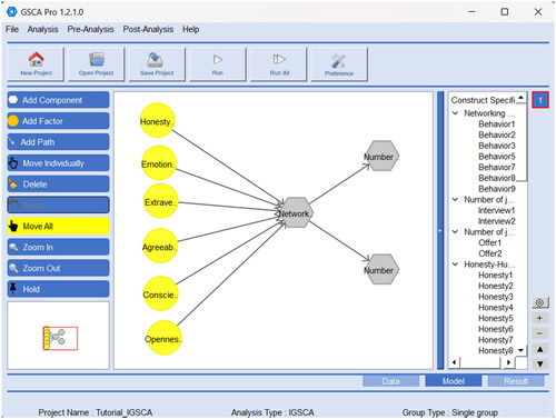
To apply IGSCA to the example, we begin by selecting Analysis → IGSCA→ Basic GSCA → single group in the GSCA Pro menu. Then, we specify the structural model as follows. We use the icon Add Factor or Add Component to include a factor or a component, respectively, in the same manner as described in the previous sections. Again, GSCA Pro displays each new factor and component as a circle and hexagon, respectively. We also specify path coefficients between factors and/or components in the same manner as described in the previous sections. We then specify the measurement model in the same way by assigning indicators to each factor/component in the Assign Indicators to Constructs window. Figure 4 displays the completed model specification in GSCA Pro, which also shows which indicators are assigned to which factor/component on the right-hand panel.

Figure 4. An illustration of applying IGSCA in GSCA Pro.

We click on the Run icon in the menu bar to fit the model to the data via IGSCA. When the IGSCA algorithm has converged, basic analysis results are provided in the Result tab. The model shows GFI = .98, SRMR = .03, and FIT = .83. As shown in Table 1, given the sample size, both GFI and SRMR values suggest an acceptable model fit. The model explains about 83% of the variance of all the factors and components and their indicators. It also shows FIT_M = .94 and FIT_S = .06, indicating that the measurement model explains 94% of the variance of all the indicators, while the structural model accounts for 6% of the variance of the factors and components.

Table 11 exhibits both factor and component loading estimates, along with their bootstrap standard errors and 95% percentile CIs. In the table, the indicators for the personality traits are rather generically labelled, e.g., Honesty1 to Honesty 10 for honesty-humility, because their exact item statements are not available. As discussed earlier, component loadings are proportional to the corresponding component weights under the unidimensional model, which are also easier to interpret. We thus focus on examining the component loading estimates. All the factor and component loading estimates are statistically significant and large in magnitude, indicating that all reflective/composite indicators are highly related to their respective factors/components.

Table 11. IGSCA’s estimates of loadings in the measurement model.

Factor/component	Indicator	Estimate	SE	95% CI
Honesty-humility	Honesty1	0.67	0.03	[0.62, 0.73]
	Honesty2	0.67	0.03	[0.62, 0.72]
	Honesty3	0.69	0.02	[0.65, 0.74]
	Honesty4	0.73	0.03	[0.69, 0.78]
	Honesty5	0.66	0.03	[0.60, 0.70]
	Honesty6	0.69	0.03	[0.62, 0.73]
	Honesty7	0.71	0.03	[0.66, 0.76]
	Honesty8	0.74	0.02	[0.70, 0.78]
	Honesty9	0.79	0.02	[0.75, 0.82]
	Honesty10	0.70	0.03	[0.65, 0.75]
Emotionality	Emotion1	0.79	0.02	[0.76, 0.82]
	Emotion2	0.81	0.02	[0.78, 0.85]
	Emotion3	0.63	0.03	[0.57, 0.69]
	Emotion4	0.64	0.03	[0.58, 0.69]
	Emotion5	0.75	0.02	[0.71, 0.80]
	Emotion6	0.61	0.03	[0.54, 0.66]
	Emotion8	0.75	0.02	[0.71, 0.79]
	Emotion10	0.71	0.03	[0.66, 0.77]
Extraversion	Extraver2	0.70	0.03	[0.63, 0.76]
	Extraver3	0.61	0.04	[0.53, 0.68]
	Extraver4	0.73	0.03	[0.67, 0.78]
	Extraver5	0.71	0.03	[0.65, 0.77]
	Extraver6	0.74	0.02	[0.70, 0.78]
	Extraver7	0.72	0.03	[0.67, 0.77]
	Extraver8	0.71	0.03	[0.65, 0.78]
	Extraver9	0.79	0.02	[0.75, 0.82]
	Extraver10	0.81	0.02	[0.76, 0.85]
Agreeableness	Agreeable1	0.82	0.02	[0.78, 0.86]
	Agreeable3	0.60	0.05	[0.51, 0.68]
	Agreeable4	0.69	0.04	[0.62, 0.77]
	Agreeable5	0.90	0.01	[0.86, 0.92]
	Agreeable7	0.88	0.02	[0.86, 0.92]
	Agreeable8	0.66	0.03	[0.58, 0.71]
	Agreeable9	0.66	0.03	[0.60, 0.72]
	Agreeable10	0.69	0.04	[0.62, 0.75]
Conscientiousness	Conscientious1	0.79	0.02	[0.72, 0.82]
	Conscientious3	0.57	0.03	[0.52, 0.62]
	Conscientious4	0.76	0.02	[0.72, 0.81]
	Conscientious6	0.72	0.03	[0.67, 0.77]
	Conscientious7	0.85	0.01	[0.82, 0.87]
	Conscientious8	0.79	0.02	[0.76, 0.83]
	Conscientious9	0.66	0.04	[0.59, 0.74]
	Conscientious10	0.61	0.04	[0.54, 0.68]
Openness to experience	Openness1	0.68	0.03	[0.61, 0.72]
	Openness2	0.70	0.03	[0.66, 0.76]
	Openness3	0.68	0.03	[0.63, 0.74]
	Openness5	0.72	0.02	[0.67, 0.76]
	Openness7	0.82	0.02	[0.78, 0.85]
	Openness8	0.66	0.03	[0.62, 0.73]
	Openness9	0.74	0.02	[0.69, 0.78]
	Openness10	0.64	0.03	[0.59, 0.70]
Networking behavior	Behavior1	0.90	0.01	[0.87, 0.93]
	Behavior2	0.80	0.02	[0.75, 0.83]
	Behavior3	0.87	0.02	[0.84, 0.90]
	Behavior5	0.73	0.02	[0.69, 0.78]
	Behavior7	0.74	0.04	[0.67, 0.80]
	Behavior8	0.91	0.01	[0.90, 0.93]
	Behavior9	0.91	0.01	[0.90, 0.93]
Number of job interviews	Interview1	0.91	0.01	[0.89, 0.92]
	Interview2	0.90	0.01	[0.89, 0.92]
Number of job offers	Offer1	0.88	0.01	[0.86, 0.90]
	Offer2	0.88	0.01	[0.86, 0.90]

Table 12 provides the path coefficient estimates and their bootstrap standard errors and 95% percentile CIs. All the personality factors have statistically significant impacts on networking behavior, i.e., honesty-humility (0.14, SE = 0.03, 95% CI = [0.08, 0.20]), emotionality (−0.43, SE = 0.03, 95% CI = [−0.50, −0.37]), extraversion (0.41, SE = 0.04, 95% CI = [0.33, 0.48]), agreeableness (0.13, SE = 0.03, 95% CI = [0.07, 0.20]), conscientiousness (0.08, SE = 0.03, 95% CI = [0.03, 0.13]), and openness to experience (0.15, SE = 0.03, 95% CI = [0.09, 0.20]). Emotionality is negatively associated with networking behavior, whereas other personality factors are positively associated. In addition, networking behavior has positive and statistically significant influences on the number of job interviews (0.13, SE = 0.04, 95% CI = [0.07, 0.21]) and the number of job offers (0.09, SE = 0.04, 95% CI = [0.02, 0.16]).

Table 12. IGSCA’s estimates of path coefficients in the structural model.

IV	DV	Estimate	SE	95% CI
Honesty-humility	Networking behavior	0.14	0.03	[0.08, 0.20]
Emotionality	Networking behavior	−0.43	0.03	[−0.50, −0.37]
Extraversion	Networking behavior	0.41	0.04	[0.33, 0.48]
Agreeableness	Networking behavior	0.13	0.03	[0.07, 0.20]
Conscientiousness	Networking behavior	0.08	0.03	[0.03, 0.13]
Openness to experience	Networking behavior	0.15	0.03	[0.09, 0.20]
Networking behavior	Number of job interviews	0.13	0.04	[0.07, 0.21]
Networking behavior	Number of job offers	0.09	0.04	[0.02, 0.16]

IV: independent variable; DV: dependent variable.

Under View Full Result, the software presents additional metrics for evaluating the model (see Table 13). For example, to evaluate the part of the measurement model that involves factors, we examine the reflective indicators’ internal consistency reliability. Both Cronbach’s α values and ρ_c values for each set of the reflective indicators are greater than 0.7 (and lower than 0.95). Also, the AVE values of the personality factors are greater than 0.5 except for Honesty-Humility (AVE = 0.5), generally speaking to their convergent validity. Furthermore, we examine the HTMT value for each pair of the six personality factors to check the factors’ discriminant validity. All the HTMT values are below the rule-of-thumb threshold of 0.9. To assess the part of the measurement model that involves components, we investigate the composite indicators’ dimensionality. We find that each component’s dimensionality is one. Also, the PVE values of the components are greater than 0.7. When we examine the VIF values of the personality factors for networking behavior, the VIF values are small (e.g., < 3). This indicates that multicollinearity is of little concern and does not inflate the standard errors of the path coefficient estimates. The f² values of the personality factors for networking behavior range from small (e.g., .02 for honesty-humility) to medium (e.g., .23 for emotionality), while the f² values of networking behavior for the numbers of job interviews (.02) and job offers (.01) are rather small.

Table 13. Additional metrics for model assessment in the IGSCA example.

	Cronbach’s α	ρC	AVE
Honesty-humility	0.91	0.91	0.50
Emotionality	0.89	0.89	0.51
Extraversion	0.91	0.91	0.53
Agreeableness	0.90	0.91	0.55
Conscientiousness	0.89	0.90	0.53
Openness to experience	0.89	0.89	0.50
	Dimensionality	PVE	R^2
Networking behavior	1	0.71	0.55
Number of job interviews	1	0.82	0.02
Number of job offers	1	0.78	0.01
IV	DV	HTMT				VIF	Effect size (f^2)
		Estimate	SE	95% CI
Honesty-humility	Networking behavior	0.28	0.04	[0.15,	0.38]	1.10	0.02
Emotionality	Networking behavior	0.57	0.04	[0.43,	0.65]	1.20	0.23
Extraversion	Networking behavior	0.47	0.04	[0.37,	0.55]	1.04	0.20
Agreeableness	Networking behavior	0.31	0.05	[0.20,	0.42]	1.06	0.02
Conscientiousness	Networking behavior	0.21	0.04	[0.11,	0.29]	1.04	0.01
Openness to experience	Networking behavior	0.28	0.04	[0.20,	0.37]	1.07	0.02
Networking behavior	Number of job interviews	0.15	0.04	[0.05,	0.25]		0.02
Networking behavior	Number of job offers	0.12	0.04	[0.02,	0.25]		0.01

4. Concluding Remarks

GSCA Pro is stand-alone software that is user-friendly and free for researchers to utilize for GSCA-SEM applications. We demonstrated how to use the software to estimate several models that included factors only, components only, and both factors and components after briefly discussing model specification, estimation, and evaluation in GSCA-SEM. The provision of these illustrations will greatly help researchers apply the software to statistically examine hypotheses about the relationships between observed variables and theoretical constructs in their research.

To our knowledge, GSCA-SEM is the most versatile SEM method in terms of accommodating the two statistical representations of constructs. As interdisciplinary research is encouraged and supported to study complex human behavior and cognition (e.g., Box-Steffensmeier et al., 2022), researchers increasingly need to consider the relationships among a greater variety of constructs emerging from diverse scientific disciplines and search for a statistical method that can handle the statistical representations of constructs in a flexible fashion. This demand will likely make GSCA-SEM a popular SEM method and GSCA Pro the software of choice for its application. We hope that this tutorial contributes to making researchers in various sciences aware of and use the method through the software.

Acknowledgment

The authors thank Marko Sarstedt for his constructive comments on an earlier version of the article.

Disclosure statement

No potential conflict of interest was reported by the authors.

Notes

1 Another version of the HTMT, termed HTMT2, was developed that relaxed the parallel assumption (Roemer et al., 2021). However, the HTMT2 requires all involved indicators to be positively correlated and is not provided in GSCA Pro.

References

- Aittomäki, A., Lahelma, E., & Roos, E. (2003). Work conditions and socioeconomic inequalities in work ability. Scandinavian Journal of Work, Environment and Health, 29, 159–165. https://doi.org/10.5271/sjweh.718
- American Psychological Association (2007). Report of the APA Task Force on Socioeconomic Status. https://www.apa.org/pi/ses/resources/publications
- Ashton, M. C., & Lee, K. (2009). The HEXACO-60: a short measure of the major dimensions of personality. Journal of Personality Assessment, 91, 340–345. https://doi.org/10.1080/00223890902935878
- Bentler, P. M., & Weeks, D. G. (1980). Linear structural equations with latent variables. Psychometrika, 45, 289–308. https://doi.org/10.1007/BF02293905
- Bollen, K. A. (1989). Structural equations with latent variables. Wiley. https://doi.org/10.1002/9781118619179
- Bollen, K. A. (2011). Evaluating effect, composite, and causal indicators in structural equation models. MIS Quarterly, 35, 359–372. https://doi.org/10.2307/23044047
- Bollen, K. A. (2019). Model implied instrumental variables (MIIVs): An alternative orientation to structural equation modeling. Multivariate Behavioral Research, 54, 31–46. https://doi.org/10.1080/00273171.2018.1483224
- Borsboom, D., Mellenbergh, G. J., & van Heerden, J. (2003). The theoretical status of latent variables. Psychological Review, 110, 203–219. https://doi.org/10.1037/0033-295X.110.2.203
- Borsboom, D., Mellenbergh, G. J., & Van Heerden, J. (2004). The concept of validity. Psychological Review, 111, 1061–1071. https://doi.org/10.1037/0033-295X.111.4.1061
- Boubker, O., & Douayri, K. (2020). Dataset on the relationship between consumer satisfaction, brand attitude, brand preference and purchase intentions of dairy product: The case of the Laayoune-Sakia El Hamra region in Morocco. Data in Brief, 32, 106172. https://doi.org/10.1016/j.dib.2020.106172
- Box-Steffensmeier, J. M., Burgess, J., Corbetta, M., Crawford, K., Duflo, E., Fogarty, L., Gopnik, A., Hanafi, S., Herrero, M., Hong, Y.-Y., Kameyama, Y., Lee, T. M. C., Leung, G. M., Nagin, D. S., Nobre, A. C., Nordentoft, M., Okbay, A., Perfors, A., Rival, L. M., … Wagner, C. (2022). The future of human behaviour research. Nature Human Behaviour, 6, 15–24. https://doi.org/10.1038/s41562-021-01275-6
- Bull, F. C., Maslin, T. S., & Armstrong, T. (2009). Global physical activity questionnaire (GPAQ): nine country reliability and validity study. Journal of Physical Activity and Health, 6, 790–804. https://doi.org/10.1123/jpah.6.6.790
- Chatterjee, S., & Price, B. (1977). Regression analysis by example. Wiley.
- Chin, W. W. (1998). The partial least squares approach for structural equation modeling. In G. A. Marcoulides (Ed.), Modern methods for business research. (pp. 295–336). Erlbaum.
- Cho, G., & Choi, J. Y. (2020). An empirical comparison of generalized structured component analysis and partial least squares path modeling under variance-based structural equation models. Behaviormetrika, 47, 243–272. https://doi.org/10.1007/s41237-019-00098-0
- Cho, G., & Hwang, H. (2023a). Deep learning generalized structured component analysis: A knowledge-based multivariate predictive method. Structural Equation Modeling: A Multidisciplinary Journal. Advance Online Publication.
- Cho, G., & Hwang, H. (2023b). Structured factor analysis: A data matrix-based alternative approach to structural equation modeling. Structural Equation Modeling: A Multidisciplinary Journal, 30, 364–377. https://doi.org/10.1080/10705511.2022.2126360
- Cho, G., Hwang, H. (2021). Generalized structured component analysis accommodating convex components. [Paper presentation] 2021 Annual Meeting of Statistical Society of Canada, Virtual Conference.
- Cho, G., Hwang, H., Sarstedt, M., & Ringle, C. M. (2020). Cutoff criteria for overall model fit indexes in generalized structured component analysis. Journal of Marketing Analytics, 8, 189–202. https://doi.org/10.1057/s41270-020-00089-1
- Cho, G., Jung, K., & Hwang, H. (2019). Out-of-bag prediction error: A cross validation index for generalized structured component analysis. Multivariate Behavioral Research, 54, 505–513. https://doi.org/10.1080/00273171.2018.1540340
- Cho, G., Sarstedt, M., & Hwang, H. (2022). A comparative evaluation of factor- and component-based structural equation modeling methods under (in)consistent model specifications. The British Journal of Mathematical and Statistical Psychology, 75, 220–251. https://doi.org/10.1111/bmsp.12255
- Cho, G., Schlaegel, C., Hwang, H., Choi, Y., Sarstedt, M., & Ringle, C. M. (2022). Integrated generalized structured component analysis: On the use of model fit criteria in international management research. Management International Review, 62, 569–609. https://doi.org/10.1007/s11575-022-00479-w
- Choi, J. Y., & Hwang, H. (2020). Bayesian generalized structured component analysis. The British Journal of Mathematical and Statistical Psychology, 73, 347–373. https://doi.org/10.1111/bmsp.12166
- Cohen, J. (1988). Statistical power analysis for the behavioral sciences. (2nd ed.). Lawrence Erlbaum Associates.
- Côté, S., Saks, A. M., & Zikic, J. (2006). Trait affect and job search outcomes. Journal of Vocational Behavior, 68, 233–252. https://doi.org/10.1016/j.jvb.2005.08.001
- Cronbach, L. J. (1951). Coefficient alpha and the internal structure of tests. Psychometrika, 16, 297–334. https://doi.org/10.1007/BF02310555
- Cronbach, L. J., & Meehl, P. E. (1955). Construct validity in psychological tests. Psychological Bulletin, 52, 281–302. https://doi.org/10.1037/h0040957
- Croon, M. (2002). Using predicted latent scores in general latent structure models. In G. A. Marcoulides & I. Moustaki (Eds.), Latent variable and latent structure models. (pp. 195–223). Erlbaum.
- Davison, A. C., & Hinkley, D. V. (1997). Bootstrap methods and their application. Cambridge University Press. https://doi.org/10.1017/CBO9780511802843
- Diamantopoulos, A., Sarstedt, M., Fuchs, C., Wilczynski, P., & Kaiser, S. (2012). Guidelines for choosing between multi-item and single-item scales for construct measurement: A predictive validity perspective. Journal of the Academy of Marketing Science, 40, 434–449. https://doi.org/10.1007/s11747-011-0300-3
- Dijkstra, T. K. (2011). Consistent partial least squares estimators for linear and polynomial factor models, https://doi.org/10.13140/RG.2.1.3997.0405
- Dijkstra, T. K. (2013). Composites as factors, generalized canonical variables revisited, https://doi.org/10.13140/RG.2.1.3426.5449
- Dijkstra, T. K. (2017). A perfect match between a model and a mode. In H. Latan & R. Noonan (Eds.), Partial least squares path modeling: Basic concepts, methodological issues and applications. (pp. 55–80). Springer. https://doi.org/10.1007/978-3-319-64069-3_4
- Dijkstra, T. K., & Henseler, J, University of Groningen (2015b). Consistent partial least squares path modeling. MIS Quarterly, 39, 297–316. https://doi.org/10.25300/MISQ/2015/39.2.02
- Dijkstra, T. K., & Henseler, J. (2015a). Consistent and asymptotically normal PLS estimators for linear structural equations. Computational Statistics and Data Analysis, 81, 10–23. https://doi.org/10.1016/j.csda.2014.07.008
- Drolet, A. L., & Morrison, D. G. (2001). Do we really need multiple-item measures in service research? Journal of Service Research, 3, 196–204. https://doi.org/10.1177/109467050133001
- Efron, B. (1979). Bootstrap methods: Another look at the jackknife. The Annals of Statistics, 7, 1–26. https://doi.org/10.1214/aos/1176344552
- Fornell, C., Johnson, M. D., Anderson, E. W., Cha, J., & Bryant, B. E. (1996). The American customer satisfaction index: Nature, purpose, and findings. Journal of Marketing, 60, 7–18. https://doi.org/10.2307/1251898
- Franke, G., & Sarstedt, M. (2019). Heuristics versus statistics in discriminant validity testing: a comparison of four procedures. Internet Research, 29, 430–447. https://doi.org/10.1108/IntR-12-2017-0515
- Götz, O., Liehr-Gobbers, K., & Krafft, M. (2010). Evaluation of structural equation models using the partial least squares (PLS) approach. In V. Esposito Vinzi, W. W. Chin, J. Henseler, & H. Wang (Eds.), Handbook of partial least squares: Concepts, methods and applications. (pp. 691–711). Springer. https://doi.org/10.1007/978-3-540-32827-8_30
- Guyon, H., Kop, J.-L., Juhel, J., & Falissard, B. (2018). Measurement, ontology, and epistemology: Psychology needs pragmatism-realism. Theory and Psychology, 28, 149–171. https://doi.org/10.1177/0959354318761606
- Hair, J. F., Ringle, C. M., & Sarstedt, M. (2011). PLS-SEM: Indeed a silver bullet. Journal of Marketing Theory and Practice, 19, 139–152. https://doi.org/10.2753/MTP1069-6679190202
- Hair, J. F., Risher, J. J., Sarstedt, M., & Ringle, C. M. (2019). When to use and how to report the results of PLS-SEM. European Business Review, 31, 2–24. https://doi.org/10.1108/EBR-11-2018-0203
- Henseler, J., Ringle, C. M., & Sarstedt, M. (2015). A new criterion for assessing discriminant validity in variance-based structural equation modeling. Journal of the Academy of Marketing Science, 43, 115–135. https://doi.org/10.1007/s11747-014-0403-8
- Hu, L., & Bentler, P. M. (1999). Cutoff criteria for fit indexes in covariance structure analysis: Conventional criteria versus new alternatives. Structural Equation Modeling: A Multidisciplinary Journal, 6, 1–55. https://doi.org/10.1080/10705519909540118
- Hwang, H., & Cho, G. (2020). Global least squares path modeling: A full-information alternative to partial least squares path modeling. Psychometrika, 85, 947–972. https://doi.org/10.1007/s11336-020-09733-2
- Hwang, H., & Takane, Y. (2004). Generalized structured component analysis. Psychometrika, 69, 81–99. https://doi.org/10.1007/BF02295841
- Hwang, H., & Takane, Y. (2014). Generalized structured component analysis: A component-based approach to structural equation modeling. Chapman and Hall/CRC Press.
- Hwang, H., Cho, G., & Choo, H. (2023). GSCA Pro for Window User’s Manual, https://doi.org/10.13140/RG.2.2.28162.61127/1
- Hwang, H., Cho, G., Jung, K., Falk, C. F., Flake, J. K., Jin, M. J., & Lee, S. H. (2021). An approach to structural equation modeling with both factors and components: Integrated generalized structured component analysis. Psychological Methods, 26, 273–294. https://doi.org/10.1037/met0000336
- Hwang, H., Desarbo, W. S., & Takane, Y. (2007). Fuzzy clusterwise generalized structured component analysis. Psychometrika, 72, 181–198. https://doi.org/10.1007/s11336-005-1314-x
- Hwang, H., Sarstedt, M., Cho, G., Choo, H., & Ringle, C. M. (2023). A primer on integrated generalized structured component analysis. European Business Review, 35, 261–284. https://doi.org/10.1108/EBR-11-2022-0224
- Hwang, H., Takane, Y., & Jung, K. (2017). Generalized structured component analysis with uniqueness terms for accommodating measurement error. Frontiers in Psychology, 8, 2137. https://doi.org/10.3389/fpsyg.2017.02137
- Jolliffe, I. T., & Cadima, J. (2016). Principal component analysis: a review and recent developments. Philosophical Transactions. Series A, Mathematical, Physical, and Engineering Sciences, 374, 20150202. https://doi.org/10.1098/rsta.2015.0202
- Jöreskog, K. G. (1971). Statistical analysis of sets of congeneric tests. Psychometrika, 36, 109–133. https://doi.org/10.1007/BF02291393
- Jöreskog, K. G. (1973). A general method for estimating a linear structural equation system. In A. S. Goldberger & O. D. Duncan (Eds.), Structural equation models in the social sciences. (pp. 255–284). Seminar Press.
- Jöreskog, K. G. (1978). Structural analysis of covariance and correlation matrices. Psychometrika, 43, 443–477. https://doi.org/10.1007/BF02293808
- Jöreskog, K. G., & Wold, H. (1982). The ML and PLS techniques for modeling with latent variables: Historical and comparative aspects. In H. Wold & K. G. Jöreskog (Eds.), Systems under indirect observation: Causality, structure, prediction, part I. (pp. 263–270). North Holland.
- Jun, Y. H., Nam, Y. H., & Ryu, J.-J. (2011). Relationships among socioeconomic status, health behavior, health status and job satisfaction. Disability and Employment, 21, 187–208.
- Jung, K., Lee, J., Gupta, V., & Cho, G. (2019). Comparison of bootstrap confidence interval methods for GSCA using a Monte Carlo simulation. Frontiers in Psychology, 10, 2215. https://doi.org/10.3389/fpsyg.2019.02215
- Kaiser, H. F. (1960). The application of electronic computers to factor analysis. Educational and Psychological Measurement, 20, 141–151. https://doi.org/10.1177/001316446002000116
- Kline, R. B. (2016). Principles and practice of structural equation modeling. (4th ed.). Guilford Press. https://psycnet.apa.org/record/2015-56948-000
- Le, S. T., & Dang, C. X. (2022). Data for the link between HEXACO personality traits and job search outcomes in Vietnam. Data in Brief, 45, 108677. https://doi.org/10.1016/j.dib.2022.108677
- Lin, S. P., & Le, S. T. (2019). Predictors and outcomes of Vietnamese university graduates’ networking behavior as job seekers. Social Behavior and Personality: An International Journal, 47, 1–11. https://doi.org/10.2224/sbp.8379
- Lohman, T. G. (1992). Advances in body composition assessment. Human Kinetics.
- MacCallum, R. C., Widaman, K. F., Preacher, K. J., & Hong, S. (2001). Sample size in factor analysis: The role of model error. Multivariate Behavioral Research, 36, 611–637. https://doi.org/10.1207/S15327906MBR3604_06
- MacCallum, R. C., Widaman, K. F., Zhang, S., & Hong, S. (1999). Sample size in factor analysis. Psychological Methods, 4, 84–99. https://doi.org/10.1037/1082-989X.4.1.84
- McArdle, J. J., & McDonald, R. P. (1984). Some algebraic properties of the reticular action model for moment structures. The British Journal of Mathematical and Statistical Psychology, 37, 234–251. https://doi.org/10.1111/j.2044-8317.1984.tb00802.x
- McNeish, D. (2018). Thanks coefficient alpha, we’ll take it from here. Psychological Methods, 23, 412–433. https://doi.org/10.1037/met0000144
- Rhemtulla, M., van Bork, R., & Borsboom, D. (2020). Worse than measurement error: Consequences of inappropriate latent variable measurement models. Psychological Methods, 25, 30–45. https://doi.org/10.1037/met0000220
- Rigdon, E. E. (2012). Rethinking partial least squares path modeling: In praise of simple methods. Long Range Planning, 45, 341–358. https://doi.org/10.1016/j.lrp.2012.09.010
- Rigdon, E. E., Sarstedt, M., & Ringle, C. M. (2017). On comparing results from CB-SEM and PLS-SEM: Five perspectives and five recommendations. Marketing ZFP, 39, 4–16. https://doi.org/10.15358/0344-1369-2017-3-4
- Roemer, E., Schuberth, F., & Jörg Henseler, J. (2021). HTMT2–an improved criterion for assessing discriminant validity in structural equation modeling. Industrial Management & Data Systems, 121, 2637–2650. https://doi.org/10.1108/IMDS-02-2021-0082
- Rönkkö, M., & Cho, E. (2022). An updated guideline for assessing discriminant validity. Organizational Research Methods, 25, 6–14. https://doi.org/10.1177/1094428120968614
- Sarstedt, M., Hair, J. F., Ringle, C. M., Thiele, K. O., & Gudergan, S. P. (2016). Estimation issues with PLS and CBSEM: Where the bias lies!. Journal of Business Research, 69, 3998–4010. https://doi.org/10.1016/j.jbusres.2016.06.007
- Sharma, P., Sarstedt, M., Shmueli, G., Kim, K. H., & Thiele, K. O. (2019). PLS-based model selection: The role of alternative explanations in information systems research. Journal of the Association for Information Systems, 20, 346–397. https://doi.org/10.17005/1.jais.00538
- Skrondal, A., & Laake, P. (2001). Regression among factor scores. Psychometrika, 66, 563–575. https://doi.org/10.1007/BF02296196
- Tenenhaus, M. (2008). Component-based structural equation modelling. Total Quality Management & Business Excellence, 19, 871–886. https://doi.org/10.1080/14783360802159543
- van der Maas, H. L. J., Kan, K.-J., & Borsboom, D. (2014). Intelligence is what the intelligence test measures. Seriously. Journal of Intelligence, 2, 12–15. https://doi.org/10.3390/jintelligence2010012
- von Zimmermann, C., Winkelmann, M., Richter-Schmidinger, T., Mühle, C., Kornhuber, J., & Lenz, B. (2020). Physical activity and body composition are associated with severity and risk of depression, and serum lipids. Frontiers in Psychiatry, 11, 494. https://doi.org/10.3389/fpsyt.2020.00494