Modeling Escherichia coli fate and transport in the Kabul River Basin using SWAT

Abstract

Access to safe water is the primary goal of all development plans, yet population increase, urbanization lead to contamination of water resources. This paper focuses on microbial contamination and aims to analyze the fate and transport of Escherichia coli in the Kabul River Basin using SWAT model to evaluate the contribution of different sources. The SWAT is calibrated and validated for the monthly time step using observed E. coli concentrations for April 2013–July 2015. The model skill score; coefficients of determination (R²) equal 0.72 and 0.70, Nash–Sutcliffe efficiencies (NSE) equal 0.69 and 0.66, and percentages bias (PBIAS) equal 3.7 and 1.9 respond well for both calibration and validation, respectively. Regional measured and modeled concentrations are very high with peaks of up to 5.2 ¹⁰log cfu/100 ml in the wet season. Overall, point sources that are comprised of human feces from the big cities and livestock manure from animal sheds, contribute most (44%) to the E. coli concentrations. During peak discharge the non-point sources become the most important contributors due to wash-off from the land and diluted point sources. Allthough such studies are lacking in developing countries, they can be helpful for sanitation management by developing and accessing regional sanitation scenarios.

Keywords:

• SWAT model
• E. coli contamination
• fate and transport
• water quality modeling
• Kabul River Basin

Introduction

Clean and safe water is indispensable for the sustenance of life. Access to safe water is the primary goal of all development plans; yet population increase coupled with industrialization, urbanization, and infrastructural limitations lead to contamination of water resources (Duan et al. 2013). Among various sources of water contamination, microbial contamination is by far the largest and probably the most serious issue in developing countries (Montgomery and Elimelech 2007). With recent improvements in living standards, water-quality aspects require more scientific support and public attention (Duan et al. 2016). Although waterborne diseases are an international issue, many people in the developing countries are extremely vulnerable due to their increased exposures and poor sanitation facilities (Cann et al. 2013; WHO 2009). The World Health Organization estimates that approximately 10% of all diseases worldwide is due to microbiologically contaminated water (Prüss-Üstün et al. 2008). In developing countries, like Pakistan, where the sanitation facilities are poor, the situation of waterborne diseases is alarming. 7% of all deaths in Pakistan are linked to waterborne issues (Azizullah et al. 2011).

Risk of waterborne diseases depends on the concentrations of waterborne pathogens in water resources (Azizullah et al. 2011). The Kabul River Basin in Pakistan is exposed to microbial contamination due to direct disposal of raw sewage from both urban and rural areas and discharge of contaminated effluents from agricultural fields. The situation is worsened by the absence of wastewater treatment plants in this basin. The contaminated surface water is used for irrigation, recreational activities, and other domestic purposes. This makes the population prone to the outbreaks of waterborne diseases (Carr and Neary 2008).

Fecal contamination in the Kabul River is not monitored and little knowledge exists on the distribution of microbes in water resources. To better understand the bacterial contamination in water resources, usually indicator organisms, such as fecal coliform and E. coli, are used to estimate the concentration of pathogenic and nonpathogenic microorganisms. Although E. coli is not directly correlated to waterborne pathogens, they have been used worldwide to indicate fecal contamination (Wu et al. 2011). This is because measuring E. coli is less expensive and time-consuming compared to other pathogenic microorganisms, such as Cryptosporidium and Rotavirus. Iqbal et al. (2017), for example, conducted large-scale sampling in the lower Kabul River Basin and observed very high concentrations of E. coli in Kabul River.

To better understand the fate and transport of microbes (pathogenic and nonpathogenic) in water resources, process-based modeling provides a low-cost and effective alternative to sampling (Shirmohammadi et al. 2006). In developing countries where waterborne diseases are endemic, process-based modeling of water quality is rare (Hofstra 2011). Hydrological models coupled with microbial modules describe the conditions in water resources considering the sources, pathways and decay of waterborne pathogens (Sokolova et al. 2013). Therefore, in this study, we implement a microbial water quality model in the highly contaminated Pakistani Kabul River Basin.

The objective of the current study is to test the model performance in an area with very high E. coli concentrations. The Soil and Water Assessment Tool was calibrated for this river basin using river discharge data from a previous study (Iqbal et al. 2018). The bacterial transport module available in SWAT (Neitsch et al. 2011; Sadeghi and Arnold 2002) is then used to simulate the fate and transport of E. coli in the catchment and to determine the main contamination sources.

Data and methods

Study site

The basic characteristics of the Kabul River Basin are described in detail by Iqbal et al. (2018). This study focusses the lower reaches of the basin, which are densely populated and prone to destructive floods. The large cities of Peshawar (2800 people per km²), Charsadda (900 people per km²), and Nowshera (1500 people per km²) are located in this area (Figure 1c). The lower Kabul River Basin covers total area of 22,000 km². A large number of livestock sheds are present in the area. Manure from these sheds is either used as fertilizer on agricultural fields or disposed directly or indirectly into the river network. The river network also carry untreated sewage effluents from urban and rural settlements to Kabul River. Microbial contamination from agricultural activities, livestock sheds and sewage disposals often result in high microbial concentrations of river. Due to such conditions and disposal practices, the number of E. coli detected in the Kabul river are 5.20 log colony forming units (cfu) per 100 ml (Iqbal et al. 2017). The land-use characteristics and soil types of the study area are presented in Table 1. The study area is in the sub-tropical zone with a mean annual precipitation of 285 mm (over the period of 2013–2015) and a mean annual surface air temperature of 22.9°C.

Figure 1. Study-area map of the lower Kabul River Basin: (a) shows the full basin along with neighboring countries. (b) Kabul basin indicating the main branches and meteorological stations, (c) shows the downstream area of Kabul basin with urban areas of Peshawar, Charsadda, and Nowshera (highlighted). Green points indicate the sampling sites from where water samples were collected, while the black triangle is the rim station where discharge is measured. At this Point Kabul River discharges into the Indus River. Sampling points Sardaryab, Shah Alam, and Amangarh are not located on the main Kabul River, but on smaller, still important, branches.

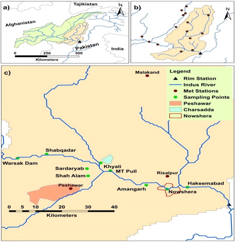
Table 1. Land-use and soil types used in the SWAT model.

Classification	Area (1000 km^−2)	Total area %
Lower Kabul Basin	22	100.0
Land-use
Crop land	8.3	34.1
Pasture/range land	5.9	24.8
Urban area	4.5	21.3
Wetland/water bodies	2.2	13.4
Barren land	0.8	6.4
Soil types
Leptosol	7.5	30.1
Rock outcrop	5.0	20.6
Fluvisol	4.3	18.4
Cambisol	2.5	15.8
Calcisol	1.4	8.5
Glaciers	1.1	6.6

Land-use types are from the European space Agency (Arino et al. 2010) and soil types are from the Harmonized World Soil Database (Nachtergaele et al. 2012).

Data

Water sampling and microbiological data

Water samples were collected from nine locations in Kabul River (see Figure 1c), the samples were analyzed for microbial concentrations through laboratory tests using the Most Probably Number approach. The sampling strategy, procedures and data are detailed in Iqbal et al. (2017). Water samples were collected between April 2013 and August 2015. The frequency of sampling during times of flooding (i.e. April to August) was daily and fortnightly samples were taken outside the flooding season. In short, samples were collected in pre-sterilized plastic bottles and transported to the laboratory of the Nuclear Institute for Food and Agriculture for bacterial analysis. For total coliform counts a series of five fermentation tubes of Mackonky broth (Merck) were inoculated with appropriate volumes of ten-fold dilutions of water samples, and incubated at 37°C for 24 h. Gas-positive tubes were considered positive for the presence of total coliform (Franson 1995). Gas-positive Mackonky broth tubes were subjected to further analysis for the confirmation of E. coli. The tubes were incubated at 44.5°C for 24 h. Each positive test tube was also exposed to an ultraviolet light lamp. Fluorescence in the tube denoted the presence of E. coli (Brenner et al. 1993). E. coli concentrations in water samples were recorded with the MPN table (WHO 1985). During flooding the E. coli concentrations ranged from 4.87 to 5.20 log cfu/100 ml and outside the flooding season the concentrations ranged from 3.61 to 4.91 log cfu/100 ml (Iqbal et al. 2017). The data were collected from sampling locations (as shown in Figure 1c) and averaged over months to calibrate the model.

Topographic, soil, land-use and climatic data

Watershed boundaries were delineated from the 90 m Digital Elevation Model data from the Shuttle Radar Topography Mission (SRTM, available through http://srtm.csi.cgiar.org). Soil data are acquired from the Harmonized World Soil Database (http://webarchive.iiasa.ac.at/Research/LUC/External-World-soil-database; Nachtergaele et al. 2012), while land use data developed by the European Space Agency for the year 2009 are used (http://due.esrin.esa.int/page_globcover.php; Arino et al. 2010) are used. The climatic data, including precipitation, minimum and maximum surface air temperature, relative humidity, solar radiation and wind speed, at a daily time step for 25 years (1981–2015) are acquired from the Pakistan Meteorological Department (PMD). Discharge data of Kabul River at Attock for the same period and time resolution were acquired from the Water and Power Development Authority (WAPDA).

Hydro-bacteriological modeling

The SWAT model is used to estimate E. coli concentrations in the Kabul River. The concentrations calculated represent the situation at Attock, which is indicated by the triangle in Figure 1c. This is the point where the Kabul River enters the Indus River. E. coli concentrations are modeled with a monthly temporal resolution.

Hydrological model

SWAT is semi-distibuted process based model that was developed to quantify the impact of management and climate on water resources, sediment and pollutant load in catchment on a continuous time scale (Abbaspour et al. 2007). Its conceptual basis operates by distributing a watershed into sub-basins. Each sub-basin is linked via stream network and further splits up into hydrological units. The model structure was built with the help of ArcGIS software, which provides graphical information of the watershed and allows for the definition of watershed hydrology.

The SWAT model was calibrated for daily discharge for 2007–2011 and validated for 2012–2015, respectively (Iqbal et al. 2018). The model evaluation statistics or skill score showed good agreement between measured and simulated results. The coefficient of determination (R²) was 0.84 and 0.77, Nash–Sutcliffe Efficiency Index (NSE) outcome was 0.77 and 0.72 and percent bias (PBIAS) values were 22.2 and 17.7 for calibration and validation time periods, respectively. Based on the model efficiency (Moriasi et al. 2007), overall the model describes the hydrological process of the watershed systems as good (Iqbal et al. 2018). The model calibrated at a daily time step has been used at the monthly resolution here. Such up scaling in time has been done before and the models perform well at both resolutions (Heathman and Larose 2007; Thampi et al. 2010).

Bacterial module

The SWAT bacterial module developed by Sadeghi and Arnold (2002) was used to predict bacterial (i.e. pathogenic and nonpathogenic) loads and concentrations in rivers. The comprehensive bacterial model considers parallel risk evaluation of bacteria loading linked with diverse land-use practices in the basin. Bacteria from each hydrological unit are collected at the sub-basin level and then moved to the watershed main outlet (Benham et al. 2006). The SWAT bacterial model simulates the fate and transport as two different bacteria populations: persistent bacteria (E. coli and other pathogens, such as Cryptosporidium) and less-persistent bacteria (fecal coliform). The persistent pathogens are considered to have lower decay rates in the natural conditions compared to less-persistent bacteria (Coffey et al. 2007; Jamieson et al. 2004). We focus solely on the persistent bacteria. To account for microbial loads in the catchment, different possible sources of bacterial pollution were included in the model, the point and non-point sources. We model monthly mean E. coli concentrations.

Human sources

The lower Kabul River Basin has over 6.2 million inhabitants living in major cities: Peshawar (2800 people per km²), Charsadda (900 people per km²), and Nowshera (1500 people per km²) and surrounding villages (Bureau of Statistics 2016). E. coli from raw sewage and domestic wastewater is discharged directly via drains, small streams, irrigation canals and other tributaries to the river, due to the absence of a wastewater treatment plants (WWTP).

The input flows from the sewage were estimated based on the number of people connected to the sewer network and water consumption per person of 95 l/day (WATSAN 2014). Each household was assumed to be occupied by four persons. We applied an effluent rate of 0.38 m³/day from each household and an effluent concentration of approximately 1.7 × 10⁶ cfu/100 ml as reported by Mara and Horan (2003), Payment et al. (2001), and Baker (1980).

Moreover, surface water resources can be polluted with microorganisms through flood water runoff from the urban settlements of Peshawar, Charsadda and Nowshera (see Figure 1c). This flood water can contain feces from animals that roam around freely or are held in small livestock sheds, such as dogs, asses, horses, and camels.

The runoff volume was simulated using the curve number method available in the SWAT model. The runoff curve number was developed by the US Department of Agriculture (USDA 1986) that is a hydrological variable to predict approximate amount of direct runoff from a precipitation event (Balvanshi and Tiwari 2014; King et al. 1999). The curve number is based on the soil type, land-use, slope and hydrologic condition. The E. coli concentrations in storm water range from 10³ to 10⁴ cfu 100 ml⁻¹ (Marsalek and Rochfort 2004). In the current study the E. coli concentration of 6.5 × 10³ cfu 100 ml⁻¹ was used and included as non-point sources in the model.

Livestock sources

Livestock manure is another important source of microbial contamination in the Kabul River Basin. Total livestock (cattle/buffalo) in the lower Kabul basin was estimated to be 0.89 million animal units (AU). The total number of sheep and goats present in the area was 1.32 and 1.15 million, respectively (Bureau of Statistics 2016). Poultry (i.e. chicken) are not included, because these are not kept in the area. The livestock is mostly housed in animal sheds. From the animal sheds the manure is used on the land, for fuel, or is dumped into the river.

The inputs of manure to water resources can be divided into indirect (via surface runoff) and direct (deposited to river) inputs. According to the American Society of Agricultural Engineer (ASAE 2005) standards, each day the manure production of cows and buffalo’s is estimated to be 27 kg of wet manure per day per 650-kg AU, which approximate equals the weight of one animal. The actual manure production by each AU may vary depending on the dietary habit of the animal. An E. coli concentration in cow/buffalo manure of 4.2*10⁵ cfu/g is used (Coffey et al. 2010) (see Table 2). That means that each cow or buffalo produces approximately 1.1 × 10¹⁰ cfu per day.

Table 2. E. coli concentration in fresh manure and waste.

Type	Animal weight (kg)	Manure production (kg day^-1)	Min (cfu/g)	Max (cfu/g)	Geometric mean (cfu/g)
Sheep/goat (Collins and Rutherford 2004; Hutchison et al. 2004; Mara and Horan 2003; Thurston-Enriquez et al. 2005)	30/50	1.3/2.5	7.8 × 10^2	1.6 × 10^7	6.6 × 10^4
Buffalo/cow (Collins and Rutherford 2004; Fegan et al. 2004; Hutchison et al. 2004; Mara and Horan 2003; Meals and Braun 2006)	650	27	2.3 × 10^5	7.5 × 10^5	4.2 × 10^5

Approximately 35 kg/ha of manure is applied monthly on the fields (crop lands) (Parmar and Sharma 2002). The remaining quarter of the manure is used as fuel, while the rest is dumped directly into the river.

Manure application

The fate and transport of the non-point source bacteria is calculated by applying manure from livestock sheds to crop land as fertilizer, adsorption to soil, extraction by runoff, decay and, finally, stream flow. The inputs and outputs of bacteria in the top soil layer can be calculated with the help of the following equation: (1) $${\Delta }_{\mathit{\text{Bact}}}\mathrm{ }={\mathit{\text{Surface}}}_{\mathit{\text{Loading}}}-{\mathit{\text{Decay}}}_{\mathit{\text{Solution}}}-{\mathit{\text{Decay}}}_{\mathit{\text{Adsorbed}}}-{\mathit{\text{Mixed}}}_{\mathit{\text{Bact}}}-{\mathit{\text{Bact}}}_{\mathit{\text{Surf}}}-{\mathit{\text{Bact}}}_{\mathit{\text{Perc}}}-{\mathit{\text{Bact}}}_{Sed}$$(1) where ${\Delta }_{\mathit{\text{Bact}}}$ is the change of bacterial loading in the top 10 mm surface soil [cfu/m²]; ${\mathit{\text{Surface}}}_{\mathit{\text{Loading}}}$ is the total bacterial loading deposited on the soil surface in one day [cfu/m²]; ${\mathit{\text{Decay}}}_{\mathit{\text{Solution}}}$ and ${\mathit{\text{Decay}}}_{\mathit{\text{Adsorbed}}}$ are the amount of bacteria in the soil solution and adsorbed to soil particles that decayed in one day [cfu/m²]; ${\mathit{\text{Mixed}}}_{\mathit{\text{Bact}}}$ is the amount of bacteria redistributed to deep soil layer by tillage [cfu/m²]; and ${\mathit{\text{Bact}}}_{\mathit{\text{Surf}}}, {\mathit{\text{Bact}}}_{\mathit{\text{Perc}}}$, and ${\mathit{\text{Bact}}}_{Sed}$ are the loadings of bacteria transported by surface runoff [mm] runoff percolating through the soil and moving sediments.

Tillage

During the tillage operation bacteria from the top 10 mm are mixed with the soil and can be lost to the lower soil layer. When bacteria reach to second layer of the soil, they become unavailable for transport via surface runoff (Ferguson et al. 2003; Muirhead et al. 2006).

Surface runoff

The movement of bacteria from the soil layer (top 10 mm) to the river with sediment is calculated as a function of the amount of bacteria attached to the sediment, the sediment yield based on runoff and the enrichment ratio for bacteria. The SWAT user manual (Neitsch et al. 2002) describes all these equations. SWAT considered direct inputs of bacteria from watershed system as point sources. Per sub-basin one point source is assigned by default. Hence, integrating all the point source from the sub-basin in the watershed by a single discharge outlet and the associated bacterial concentration is important. This is usually done at the main outlet of the watershed.

The movement of bacteria from the soil solution of the soil layer (top 10 mm) to the river due to surface runoff is a function of runoff amount and soil bacteria contact. The SWAT model simulates the bacterial transport during surface runoff similar to the soluble phosphorus movement and is based on pesticide equations suggested by Leonard and Wauchope (Knisel 1980; Pierson et al. 2001). The strength of this association is embedded in the bacteria-soil partitioning coefficient (BACTKDQ): (2) $${\mathit{\text{Bact}}}_{\mathit{\text{Surf}}}=\frac{{\mathit{\text{Bact}}}_{\mathit{\text{solution}}}\mathrm{ }\mathrm{*}{\mathrm{ }Q}_{\mathit{\text{surf}}}\mathrm{ }}{P\beta \text{ * }\mathit{\text{depth}}\text{ * }\mathit{\text{BACTKDQ}}}$$(2) where ${\mathit{\text{Bact}}}_{\mathit{\text{Surf}}}$is the bacterial amount transported through runoff [cfu/m²], ${\mathit{\text{Bacteria}}}_{\mathit{\text{solution}}}$ is a number of bacteria in the top 10mm of soil layer [cfu/m²], ${ Q}_{\mathit{\text{surf}}}$ is the volume of surface runoff [mm], $P\beta$ is the bulk density [mg/m³], and $\mathit{\text{BACTKDQ}}$ is the bacterial-soil partitioning coefficient [m³/mg]. $\mathit{\text{BACTKDQ}}$ is expected to be independent from the type of bacteria simulated by the SWAT model, land-use and soil type. There is no range of values given for this variable. The SWAT model took 175 for phosphorus as default (Neitsch et al. 2002), however, the value is 100 in the Agricultural Policy Extender (APEX) model (Williams et al. 2008). Therefore, the value between 100 and 200 is a rational start for the calibration of bacterial movement.

Upstream inputs

Another important source of bacterial contamination in the lower part of the Kabul River Basin is the input bacterial load from upstream part (above Warsak Dam, see Figure 1c) of the river. The observed concentrations at the Warsak sampling point have been used as input into the model.

River concentrations

In the river the bacteria mass balance is presented by the following equation: (3) $${\Delta }_{\mathit{\text{Stream}}-\mathit{\text{bact}}}={\mathit{\text{Bact}}}_{\mathit{\text{Surf}}}-{\mathit{\text{Bact}}}_{Sed}+{\mathit{\text{Direct}}}_{\mathit{\text{Inputs}}}-{\mathit{\text{Decay}}}_{\mathit{\text{Stream}}}-{\mathit{\text{Bact}}}_{\mathit{\text{Flow}}}$$(3) where ${\Delta }_{\mathit{\text{Stream}}-\mathit{\text{bact}}}$ is the change of bacteria loading in stream in one day [cfu/m²]; ${\mathit{\text{Bact}}}_{\mathit{\text{Surf}}}\text{ and }{\mathit{\text{Bact}}}_{Sed}$ are the loadings of bacteria [cfu/m²] in solution and adsorbed to soil particles transported by surface runoff [mm]. ${\mathit{\text{Direct}}}_{\mathit{\text{Inputs}}}$ are the bacteria loading directly discharged in to river by wastewater treatment plant (if any); ${\mathit{\text{Decay}}}_{\mathit{\text{Stream}}}$ is the number of bacteria decayed during one day [cfu/m²], and ${\mathit{\text{Bact}}}_{\mathit{\text{Flow}}}$ is the number of bacteria transported out of reach by stream flow [cfu/m²].

Decay

Bacteria are considered to be dissolved pollutants and changes in the river concentration can be calculated with the first-order decay equation (chick’s law) proposed by Mancini (1978) and revised by Moore et al. (1989) to model fecal bacteria decay. Decay rates can be determined with the following equation. (4) $$C_{t\mathrm{ }}=\mathrm{ }{C}_0\mathrm{ }\mathrm{*}\mathrm{ }{e}^{-k_{20}{t}_{\theta }\mathrm{ }{\mathrm{*}}^{\left(T-20\right)}}$$(4) where C_t is the bacterial concentration in the river at time t, [count per 100 ml] C₀ is the initial bacterial concentration [count per 100 ml] K₂₀ is the first order die off rate at 20°C [per day] t is the exposure time in [days] $t\mathrm{\theta }$ is temperature adjustment factor (THBACT in SWAT model), T is expressing ambient temperature [°C]. Both $t\mathrm{\theta }$ and${ K}_{20}$ are user specified. In SWAT K₂₀ is specified to be 20°C per day for E. coli. Reddy et al. (1981) described the decay rates for fecal coliforms and fecal streptococci (i.e. the average die-off rates were 1.14 and 0.41 per day, respectively). They also described that microbial die-off increased with decrease in soil moisture, pH (range of 6–7) and with 10°C rise in temperature the die-off rates increased approximately two times.

Model calibration procedures

The SWAT bacterial module was calibrated (April 2013 to June 2014) and validated (August 2014 to July 2015) for monthly mean E. coli concentration. The SWAT bacterial model was calibrated with the SWAT Calibration Uncertainties Program (SWAT-CUP) (Abbaspour 2015) while using the Sequential Uncertainty Fitting version 2 (SUFI-2) algorithm (Abbaspour et al. 2004, 2007). To determine the variables that need to be calibrated, the variables to which the E. coli concentrations are most sensitive were included in a sensitivity analysis. A one-factor-at-a-time (Hogan et al. 2012) sampling method Morris (1991), was applied in the Sequential Uncertainty Fitting SUFI-2 algorithm SWAT-CUP automatic sensitivity analysis tool (Abbaspour 2012). This robust method has been extensively used in modeling, despite its long calculation times (Van Griensven et al. 2002). The sensitivity analysis was also performed to evaluate how the simulated output was influenced by the input variables. To that extent, individual variables were changed by 10% of the initial value (keeping all other input variables constant), and the effect on the E. coli concentration was examined. For the calibration of the model, the values of the most sensitive variables were adjusted between ranges that were preset in the SWAT model and are based on earlier worldwide studies. The optimum values were set and subsequently used in the model. For validation, the simulated output was compared with measured E. coli data. Model evaluation statistics were calculated during both calibration and validation.

Model evaluation statistics

The model evaluation statistics or skill score were carefully chosen so that they were (1) robust to several models and climatic conditions and (2) established and recommended in available literature (Moriasi et al. 2007). Model evaluation statistics used to evaluate the measured versus predicted data includes the coefficient of determination (R²), Nash–Sutcliffe Efficiency (NSE) and percent bias (PBIAS). The coefficient of determination (R²) values shows how measured versus predicted values track a best-fit line. This R² can range from zero (no correlation) to one (perfect correlation) (Maidment 1993). The Nash–Sutcliffe Efficiency Index (NSE) indicates how reliably measured values matched with predicted values (Nash and Sutcliffe 1970). This index ranges from negative infinite (poor) to 1.0 (perfect model). The NSE values have been widely used for the assessment of hydrological models (Wilcox et al. 1990). Generally, model simulations are called satisfactory when NSE >0.50, R² > 0.60, and −25% < PBIAS <25%. Negative values of PBIAS indicate that the model overestimates flow while positive values of PBIAS indicate underestimated flow (Gupta et al. 1999). Moriasi et al. (2007) categorized the model capabilities as excellent (NSE ≥0.90), very good (NSE = 0.75–0.89), good (NSE = 0.50–0.74), fair (NSE = 0.25–0.49), poor (NSE = 0.0–0.24), and unsatisfactory if (NSE <0.0).

Results

Bacterial calibration and validation

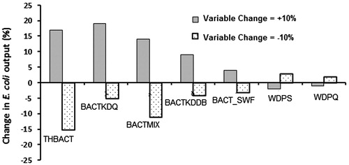
The bacterial model was sensitive to 12 variables. These have been calibrated according to the values in Table 3. The outcome of sensitivity analysis shows that the precise value of these variables can considerably affect model outcome. For example, the bacteria-soil partitioning coefficient (BACTKDQ), the bacterial percolation coefficient (BACTMIX) and the temperature adjustment factor for die-off (THBACT) are the most sensitive variables that affect E. coli concentrations. The result of sensitive analysis are shown in Figure 2. When the value of THBACT is increased or decreased by 10%, the overall model output was changed by +17% and −15%, respectively. The other two variables were similarly sensitive.

Figure 2. E. coli concentration calibration and validation results for Kabul river basin.

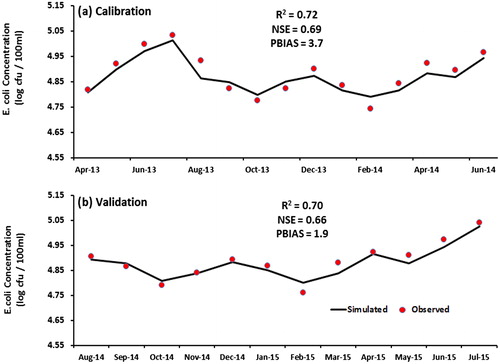
Table 3. Selected variables and their final calibrated values for the SWAT-Model to simulate E. coli concentrations.

Variables	Range of values	Fitted value
Bacterial Percolation Coefficient (BACTMIX)	7–20	16.42
Bacteria Soil Partition Coefficient ( BACTKDQ)	150–200	177.17
Bacterial partition coefficient in manure (BACTKDDB)	0–1	0.79
Die-off factor for persistent bacteria in soil Solution (per day; WDPQ)	0–1	0.41
Die-off factor for persistent bacteria adsorbed to soil particles (per day; WDPS)	0–1	0.74
Fraction of manure applied to land areas that have active colony forming units (BACT_SWF)	0–1	0.89
Growth factor for persistent bacteria in soil solution (per day; WGPQ)	0–1	0.47
Growth factor for persistent bacteria absorbed to soil particles (per day; WGPS)	0–1	0.33
Groundwater delay (GW_DELAY)	30–100	41.93
Minimum daily bacteria loss for persistent bacteria (BACTMINP)	0–5	3.15
Saturated hydraulic conductivity (SOL_K)	0–4	1.37
Temperature adjustment factor for bacteria Die-off/growth (THBACT)	1–1.18	1.08

The coefficients of determination (R²) are 0.72 and 0.70, Nash–Sutcliffe Efficiency Index (NSE) are 0.69 and 0.66 and the percent bias (PBIAS) for the bacterial model are 3.7 and 1.9 for calibration and validation, respectively. This means that the performance of the model can be classified as good. The outcome of the simulated monthly values were compared with averaged monthly observed values for E. coli (Figure 3). The SWAT model overall produces results with slightly too low variability. This is a standard artifact seen in microbiological modeling. In general, the trend in model predictions follows the observed patterns and the values showed good agreement between simulated and measured E. coli concentrations.

Figure 3. Sensitivity analysis results for the E. coli simulations, where THBACT is the temperature adjustment factor; BACTKDQ is the bacteria partition coefficient in surface runoff; BACTMIX is the bacterial percolation coefficient; BACTKDDB is the bacterial partition coefficient in manure; BACT_SWF is the fraction of manure applied to land; WDPS is the die-off factor for persistent bacteria adsorbed to soil particles; and WDPQ is the die-off factor for persistent bacteria in soil solution.

E. coli source estimation

Figure 3 shows that the monthly mean E. coli concentrations in Kabul River are high. They range from 6.5*10⁴ to 1.1*10⁵ cfu/100 ml. This water is certainly unsuitable for bathing. The concentrations strongly exceed the US-EPA daily (single sample) bathing water quality standards of 235 cfu/100 ml. Concentration peaks were observed during the flooding months of April to August 2013, 2014, and 2015.

To estimate the contributions of contamination sources to the overall E. coli concentrations, point and non-point sources of contaminations were simulated separately and their share in the total load was calculated for the total simulation period (April 2013 to September 2015). 44% of total E. coli concentration originates from the point source in the watershed.

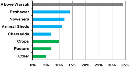
Non-point sources contribution accounts for 22% and E. coli loads from above Warsak account for 34% of the total loads in the watershed system (Figure 4). The point sources include untreated sewage and direct deposition of manure. The major point source of pollution is sewage from Peshawar (14%) followed by sewage from Nowshera (12%) and manure from Amangarh (11%). Also the contribution from Charsadda is substantial (7%). Crops and pasture are the most important non-point sources at 10% and 7%, respectively. Flood water runoff was included in the model as non-point source and contributes 5%.

Figure 4. The share of E. coli sources from upstream and downstream areas of Kabul River basin in the E. coli load. The blue color shows the E. coli concentrations from point sources including animal sheds and human settlements. The green color shows the E. coli concentrations from non-point sources and the gray area represents the load from above Warsak (upstream settlements that contribute point and non-point sources).

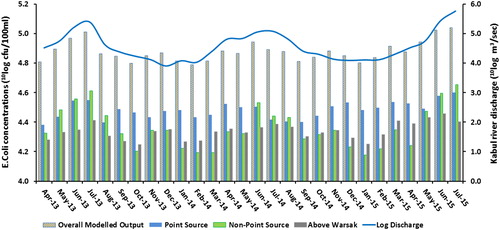
The concentration and also the contribution from the sources varies over the study period (Figure 5). The relative contribution of non-point sources is higher in flooding months (April–August). The reason for that is high precipitation increases the runoff of manure from the fields. In these cases this effect weighs up to the dilution that could also occur with increased precipitation and flow. At times of non-flooding, the chances of surface runoff from agricultural land are reduced due to low precipitation that increases the contribution from point sources due to constant input load to the river.

Figure 5. The overall E. coli concentration in Kabul River along with the river discharge specified for above Warsak, point source and non-point source contributions.

Discussion

In this paper, we modeled the E. coli concentrations in Kabul River water and analyzed the contribution of contamination sources. The SWAT model was used in this study. The most sensitive variables in this study were the bacteria-soil partitioning coefficient (BACTKDQ), the bacterial percolation coefficient (BACTMIX), and the temperature adjustment factor for die-off (THBACT). These variables were calibrated together with nine other variables.

Model validation showed that the model performs well. The NSE values for monthly E. coli concentrations were 0.69 and 0.66 for calibration and validation, respectively. Other studies using the SWAT model find similar NSE values, although these are not always fully comparable due to different temporal resolutions and the use of a more generic fecal coliform bacteria. Benham et al. (2006), for example, find NSE values of 0.63 and 0.61 for their calibration and validation period for monthly fecal coliform bacteria for the Shoal Creek Watershed in Missouri; US. Chin et al. (2009) find an NSE of 0.73 for daily E. coli concentrations in an experimental watershed in Georgia, US; and Parajuli et al. (2009) find NSE values from -2.92 to 0.71 for daily source-specific fecal coliform bacteria concentrations in the Upper Wakarusa watershed in Kansas, US. Coffey et al. (2010) applied the SWAT model to predict the transport of E. coli and found NSE values from 0.78 to 0.59 at Fergus catchment in Ireland. Similarly, Coffey et al. (2013) also applied the SWAT model and find NSE values from -0.42 to - 0.29 for daily E. coli concentrations at Kilshanvey catchment at Ireland. Bougeard et al. (2011) coupled the SWAT model with hydrodynamic model MARS 2D to predict the E. coli concentrations at the Daoulas catchment in France. They found R² of 0.99 for river water quality and 0.89 for shellfish quality. Kim et al. (2010) also applied the SWAT model to predict streambed E. coli concentrations released and deposited on sediment re-suspension at Little Cove Creek watershed in Pennsylvania. They found that surface runoff carried large numbers of E. coli to the river. Our study is, as far as we are aware, the first one on microbial modeling with the SWAT model in a developing subtropical country. The comparison above shows that our calibration and validation results are satisfactory and the modeling outcomes are reliable.

The Kabul River contains very high E. coli concentrations. It can be classified as ‘grossly polluted’ (Medema et al. 2009) with all observed and simulated values larger than 10,000 cfu/100 ml. US-EPA’s (2001) single sample bathing water quality standard (235 cfu/100 ml for E. coli) is strongly violated year around. The simulated and observed results presented considerable spatiotemporal variations. The highest concentrations peaks were observed at times of monsoon (June to August) with associated high surface-air temperature that causes snow/glacier melt and flooding. While the concentration in January and February is around 3.8 ¹⁰log cfu/100 ml, the peak concentrations reach up to 5.2 ¹⁰log cfu/100 ml in August. This suggests that peak concentrations of E. coli appear during substantially high flow due to increased surface runoff from land to water resources in the lower Kabul River basin. Modeling thus enables us to better understand the source of these higher concentrations. In some months with high concentrations (e.g. June–August 2013, 2014, and 2015), the non-point sources contributed relatively more to the total loads as during these months monsoon precipitation coincides with snow and glacier melt that causes floods. While, in other months point sources appear to contribute more because of constant load to river. Higher microbiological concentrations during monsoon periods (i.e. high precipitation events) and high river flow (due to snow/glacier melt) were also observed in other studies (Ouattara et al. 2013; Schilling et al. 2009). The reason for this is that high precipitation increases the runoff of manure from the fields. In these cases this effect weighs up to the dilution that could also occur with increased precipitation and flow. An important mechanism t in these regions is that flooding of agricultural land will wash large amounts of manure into the river. Our modeled peaks could thus be a slight underestimate. At times of non-flooding, the chances of surface runoff from agricultural land are reduced because of low precipitation. Meanwhile, a constant input of bacterial loads from cities and livestock sheds occurs and this increases the contribution from point sources to the river.

These outcomes showed that, overall, total loads from direct sewage and manure discharges and upstream concentrations (i.e. above Warsak) contributed most to the total concentrations (34% and 44%, respectively; Figure 2). Chin et al. (2009) also found high concentrations of fecal coliforms in a river in Georgia, US, due to direct inputs of pollutants. Diffuse emissions were less important, although they still contributed around 22%. Comparatively lower contribution from non-point sources was also observed by others (Ouattara et al. 2013; Sokolova et al. 2012).

The loads from Peshawar contribute most out of the point sources. The population of Peshawar is large (3.13 million people) and nearly everyone is connected to the sewer. Unfortunately, the wastewater treatment plant has been broken since the extreme 2010 flood. Also, Nowshera and Charsadda (1.77 and 1.37 million people, respectively) are large cities without functioning wastewater treatment systems. The animal sheds in the basin, which are mostly located in Amangarh (see Figure 1c), also strongly contribute to the total concentrations. Livestock numbers in the basin are large (0.89 million) and especially cows emit relatively large amounts of E. coli in their manure. Approximately 20% of total manure collected from livestock sheds is used on the land and 25% is sold as fuel, about 55% of this manure is deposited on the river side and enters the river quickly (Nisar et al. 2003).

Modeling studies have inherent uncertainties. For instance, some processes could be omitted, calibrations may not provide as satisfying results as hoped for, or input data are lacking. The SWAT model performs fine for the Kabul River Basin. However, Figure 3 shows that the model slightly overestimates low concentrations and underestimates high concentrations. The lower estimates of peak concentrations are directly related to the too low estimate of peak discharge, as explained in (Iqbal et al. 2018). Such low estimate is standard in hydrological modeling (Döll et al. 2003). The low underestimates of peak concentrations could also be partly related to the free moving animals in the basin, such as dogs, asses, camels and horses. These animals are present, but limited in numbers and precise data are not available. During extreme precipitation events more of their excreta may reach the river. In urban areas these animals have been included in an urban runoff fraction. However, these are ignored in rural areas. As the numbers of these animals are generally low in the basin, excluding them in the current study should not affect our outcomes substantially. The too high estimates of the low flow could cause by a too high overestimate of the direct inputs of sewage. Although the sewage is not treated, it does have a long residence time in the drains and the irrigation canals and during this period decay can occur. Similarly, the manure from the animal sheds will stay on the river banks for a while before it enters the river. Also then decay can occur. The assumptions that we have used in this model, are based on available data and insights. The model quality can be classified as good and therefore the results are likely robust.

The microbial water quality in Kabul River is very poor. While the population does like to bathe in the river or use the water for other purposes, the water is not safe to do so. Together with E. coli, other pathogens will be present and these can cause disease. Thorough sewage and manure management is thus required to improve this situation. The provincial government of Khyber Pukhtunkhwa, Pakistan (EPA-KP 2014) has already started to reconstruct and establish new wastewater treatment plants for cities. Treatment will also become compulsory for other urban settlements and industries. To better understand the sources of the poor water quality and its high health risks, and to assess the impact of interventions, modeling provides opportunities. The SWAT bacterial model developed in this study could be a dependable assessment tool that can be used by water and public health managers to obtain information in controlling the widespread microbiological contamination of Kabul River.

Conclusions

The objective of this study was to analyze the fate and transport of E. coli in the lower Kabul River Basin and to provide improved understanding of the influence of different processes involved in E. coli’s transport to water resources. The highly sensitive variables for pathogen modeling, BACTKDQ, BACTMIX and THBACT, show that the presence of E. coli likely lead to higher E. coli concentrations at the watershed outlet. The model performance was good. High and low concentrations were slightly underestimated. Mean monthly E. coli concentrations were high and range from 6.5*10⁴ to 1.1*10⁵ cfu/100 ml. Point source of contamination contributed to 44%. Non point souces contribution accounted for approximately 22% while E. coli from above Warsak accounted for 34% of the total conentration in the watershed system. E. coli concentration peaks were observed during the flooding months of July–August 2013, 2014 and 2015. To improve the surface water quality in Kabul River, the focus should thus be on wastewater treatment and prevention of the direct manure loads from livestock sheds.

Based on the outcomes of this modeling study, the upstream concentrations and point source of microbial pollution were found to be the major contributor in contaminating the surface-water resources in the Kabul River Basin. The developed model could be useful in future studies on assessing the impacts of socioeconomic developments and climate change on E. coli concentrations. Such modeling study can provide useful information to water managers to improve the surface-water quality and to protect humans from waterborne diseases, which still are the leading cause of death in developing countries like Pakistan.

Acknowledgments

The authors would like to acknowledge Nuffic (NFP), Government of the Netherlands for providing the Ph.D. fellowship. Thanks to Professor Dr. Raghavan Srinivasan and Dr. Karim Abbaspour for their support of the SWAT model setup and variables selection for pathogen modeling. Special thanks to Professor Dr Rik Leemans (Wageningen University and Research) and Confidence Duku for critical review and correction of this manuscript.

Disclosure statement

The authors declare no conflict of interest. The founding sponsors had no role in the design of the study; in the collection, analysis, or interpretation of data; in the writing of the manuscript, and in the decision to publish the results.

References

- Abbaspour K. 2012. Swat-Cup 2012: Swat Calibration and Uncertainty Programs – A User Manual EAWAG. Swiss Federal Institute of Aquatic Science and Technology, Zurich, Switzerland
- Abbaspour K, Yang J, and Reichert P, et al. 2008. Swat-cup, swat calibration and uncertainty programs. Swiss Federal Institute of Aquatic Science and Technology (EAWAG), Zurich, Switzerland
- Abbaspour K, Johnson C, and Van Genuchten MT. 2004. Estimating uncertain flow and transport parameters using a sequential uncertainty fitting procedure. Vadose Zone J 3:1340–52
- Abbaspour KC, Yang J, and Maximov I, et al. 2007. Modelling hydrology and water quality in the pre-alpine/alpine thur watershed using swat. J Hydrol 333:413–30
- Arino O, Ramos J, and Kalogirou V, et al. 2010. Globcover 2009. http://due.Esrin.Esa.Int/files/globcover2009_validation_report_2.2.Pdf. Accessed 10 May 2016
- ASAE. 2005. Manure production and characteristics. (Americal Society of Agricultural Engineering). St. Joseph Michigan, USA.health–a review. Environ Int 37:479–97
- Azizullah A, Khattak MN, and Richter P, et al. 2011. Water pollution in Pakistan and its impact on public health – a review. Environ Int 37:479–97
- Baker J. 1980. Agricultural areas as nonpoint sources of pollution. Agricultural Areas as Nonpoint Sources of Pollution 275–311
- Balvanshi A, and Tiwari HL. 2014. A comprehensive review of runoff estimation by the curve number method. Int J Innov Res Sci Eng Technol 3:17480–5
- Benham BL, Baffaut C, Zeckoski RW, et al. 2006. Modeling bacteria fate and transport in watersheds to support tmdls. Trans ASABE 49:987–1002
- Bougeard M, Le Saux JC, and Pérenne N, et al. 2011. Modeling of Escherichia coli fluxes on a catchment and the impact on coastal water and shellfish quality1. JAWRA Journal of the American Water Resources Association 47:350–66
- Brenner KP, Rankin CC, and Roybal YR, et al. 1993. New medium for the simultaneous detection of total coliforms and Escherichia coli in water. Appl Environ Microbiol 59:3534–44
- Bureau of Statistics. 2016. Khyber Pukhtoonkhwa Bureau of Statistics. http://kpbos.Gov.Pk/. Accessed 18th July 2016. Khyber Pukhtoonkhwa
- Cann K, Thomas DR, Salmon R, et al. 2013. Extreme water-related weather events and waterborne disease. Epidemiol Inf 141:671
- Carr GM, and Neary JP. 2008. Water quality for ecosystem and human health. International Institute PAS, Europe: UNEP/Earthprint
- Chin DA, Sakura-Lemessy D, and Bosch DD, et al. 2009. Watershed-scale fate and transport of bacteria. ASABE 52:145–54
- Coffey R, Cummins E, and Bhreathnach N, et al. 2010. Development of a pathogen transport model for Irish catchments using swat. Agric Water Manage 97:101–11
- Coffey R, Cummins E, and Cormican M, et al. 2007. Microbial exposure assessment of waterborne pathogens. Hum Ecol Risk Assess 13:1313–51
- Coffey R, Dorai-Raj S, and O’Flaherty V, et al. 2013. Modeling of pathogen indicator organisms in a small-scale agricultural catchment using swat. Hum Ecol Risk Assess Int J 19:232–53
- Collins R, and Rutherford K. 2004. Modelling bacterial water quality in streams draining pastoral land. Water Research 38:700–12
- Döll P, Kaspar F, and Lehner B. 2003. A global hydrological model for deriving water availability indicators: model tuning and validation. J Hydrol 270:105–34
- Duan W, He B, and Nover D, et al. 2016. Water quality assessment and pollution source identification of the eastern Poyang lake basin using multivariate statistical methods. Sustainability 8:133
- Duan W, Takara K, and He B, et al. 2013. Spatial and temporal trends in estimates of nutrient and suspended sediment loads in the Ishikari River, Japan, 1985 to 2010. Sci Total Environ 461–462:499–508
- EPA-KP. 2014. An Act to Provide for the Protection, Conservation, Rehabilitation and Improvement of the Environment, for the Preventation and Control of Pollution, and Promotion of Sustainable Development in the Province of the Khyber Pakhtunkhwa. Government Press, Khyber Pukhtunkhwa, Provincial Assembly KP
- Fegan N, Vanderlinde P, and Higgs G, et al. 2004. The prevalence and concentration of escherichia coli o157 in faeces of cattle from different production systems at slaughter. Journal of applied microbiology 97:362–70
- Ferguson C, Husman AMdR, and Altavilla N, et al. 2003. Fate and transport of surface water pathogens in watersheds. Critical reviews in environmental science and technology 33:299–311
- Franson MAH. 1995. American public health association American water works association water environment federation. Methods 6:84
- Gupta HV, Sorooshian S, and Yapo PO. 1999. Status of automatic calibration for hydrologic models: comparison with multilevel expert calibration. J Hydrol Eng 4:135–43
- Heathman G and Larose M. Influence of scale on swat model calibration for streamflow. In: Proceedings of the MODSIM 2007 International Congress on Modelling and Simulation, Christchurch, New Zealand, 2007, pp 2747–53
- Hofstra N. 2011. Quantifying the impact of climate change on enteric waterborne pathogen concentrations in surface water. Curr Opin Environ Sustain 3:471–9
- Hogan JN, Daniels ME, and Watson FG, et al. 2012. Longitudinal Poisson regression to evaluate the epidemiology of cryptosporidium, giardia, and fecal indicator bacteria in coastal California wetlands. Appl Environ Microbiol 78:3606–13
- Hutchison M, Walters L, and Avery S, et al. 2004. Levels of zoonotic agents in british livestock manures. Letters in Applied Microbiology 39:207–14
- Iqbal MS, Ahmad MN, and Hofstra N. 2017. The relationship between hydro-climatic variables and E. coli concentrations in surface and drinking water of the Kabul river basin in Pakistan. AIMS Environ Sci 4:690–708
- Iqbal MS, Dahri ZH, and Querner EP, et al. 2018. Impact of climate change on flood frequency and intensity in the Kabul river basin. Geosciences 8:114
- Jamieson R, Gordon R, and Joy D, et al. 2004. Assessing microbial pollution of rural surface waters: a review of current watershed scale modeling approaches. Agric Water Manage 70:1–17
- Kim J-W, Pachepsky YA, and Shelton DR, et al. 2010. Effect of streambed bacteria release on E. coli concentrations: monitoring and modeling with the modified swat. Ecol Model 221:1592–604
- King KW, Arnold J, and Bingner R. 1999. Comparison of green-ampt and curve number methods on goodwin creek watershed using swat. Trans ASAE 42:919–25
- Knisel W. 1980. A Field Scale Model for Chemical, Runoff, and Erosion from Agricultural Management Systems. Conservation Service Report 26. US Department of Agriculture, Washington, DC
- Maidment DR. 1993. Handbook of Hydrology. The University of Michigan, McGraw-Hill Inc
- Mancini JL. 1978. Numerical estimates of coliform mortality rates under various conditions. J Water Pollut Control Fed 50:2477–84
- Mara D and Horan NJ. 2003. Handbook of Water and Wastewater Microbiology. Academic Press, Great Britain
- Marsalek J and Rochfort Q. 2004. Urban wet-weather flows: sources of fecal contamination impacting on recreational waters and threatening drinking-water sources. J Toxicol Environ Health A 67:1765–77
- Meals DW, and Braun DC. 2006. Demonstration of methods to reduce runoff from dairy manure application sites. Journal of environmental quality 35:1088–100
- Medema G, Teunis P, and Blokker M, et al. 2009. Risk Assessment of Cryptosporidium in Drinking-Water (World Health Organization). WHO/HSE/WSH/09.04. World Health Organization, Geneva
- Montgomery MA and Elimelech M. 2007. Water and sanitation in developing countries: including health in the equation. Environ Sci Technol 41:17–24
- Moore J, Smyth J, and Baker E, et al. 1989. Modeling bacteria movement in livestock manure systems. Trans ASAE 32:1049–53
- Moriasi DN, Arnold JG, and Van Liew MW, et al. 2007. Model evaluation guidelines for systematic quantification of accuracy in watershed simulations. Trans ASABE 50:885–900
- Morris MD. 1991. Factorial sampling plans for preliminary computational experiments. Technometrics 33:161–74
- Muirhead RW, Collins RP, and Bremer PJ. 2006. Interaction of Escherichia coli and soil particles in runoff. Appl Environ Microbiol 72:3406–11
- Nachtergaele F, van Velthuizen H, and Verelst L, et al. 2012. Harmonized world soil database, version 1.2, fao, iiasa, isric, isscas, jrc
- Nash JE and Sutcliffe JV. 1970. River flow forecasting through conceptual models part i – a discussion of principles. J Hydrol 10:282–90
- Neitsch S, Arnold J, and Kiniry J, et al. 2002. Soil and Water Assessment Tool User’s Manual Version 2000 (GSWRL Report). Texas Water Resource Institute, Texas, USA
- Neitsch SL, Arnold JG, and Kiniry JR, et al. 2011. Soil and Water Assessment Tool Theoretical Documentation Version 2009. Texas Water Resources Institute, Texas, USA
- Nisar A, Rashid M, and Vaes AG. 2003. Fertilizers and Their Use in Pakistan. Extension Bulletin. National Fertilizer Development Centre, Planning and Development Division, Government of Pakistan, Pakistan
- Ouattara NK, and de Brauwere A, and Billen G, et al. 2013. Modelling faecal contamination in the scheldt drainage network. J Mar Syst 128:77–88
- Parajuli PB, Mankin KR, and Barnes PL. 2009. Source specific fecal bacteria modeling using soil and water assessment tool model. Bioresource Technol 100:953–63
- Parmar D, and Sharma V. 2002. Studies on long-term application of fertilizers and manure on yield of maize-wheat rotation and soil properties under rainfed conditions in western-Himalayas. J Ind Soc Soil Sci 50:311–2
- Payment P, Plante R, and Cejka P. 2001. Removal of indicator bacteria, human enteric viruses, giardia cysts, and cryptosporidium oocysts at a large wastewater primary treatment facility. Can J Microbiol 47:188–93
- Pierson S, Cabrera M, and Evanylo G, et al. 2001. Phosphorus losses from grasslands fertilized with broiler litter: EPIC simulations. J Environ Qual 30:1790–5
- Prüss-Üstün A, Bos R, and Gore F, et al. 2008. Safer Water, Better Health: Costs, Benefits and Sustainability of Interventions to Protect and Promote Health. World Health Organization
- Reddy K, Khaleel R, and Overcash M. 1981. Behavior and transport of microbial pathogens and indicator organisms in soils treated with organic wastes. J Environ Qual 10:255–66
- Sadeghi AM and Arnold JG. A swat/microbial sub-model for predicting pathogen loadings in surface and groundwater at watershed and basin scales. In: Proceedings of the Total Maximum Daily Load (TMDL): Environmental Regulations, Proceedings of 2002 Conference, 2002, American Society of Agricultural and Biological Engineers, pp 56–63
- Schilling KE, Zhang Y-K, and Hill DR, et al. 2009. Temporal variations of Escherichia coli concentrations in a large midwestern river. J Hydrol 365:79–85
- Shirmohammadi A, Chaubey I, and Harmel R, et al. 2006. Uncertainty in tmdl models. Trans ASAE 49:1033–49
- Sokolova E, As̊tröm J, and Pettersson TJR, et al. 2012. Estimation of pathogen concentrations in a drinking water source using hydrodynamic modelling and microbial source tracking. J Water Health 10:358–70
- Sokolova E, Pettersson TJR, and Bergstedt O, et al. 2013. Hydrodynamic modelling of the microbial water quality in a drinking water source as input for risk reduction management. J Hydrol 497:15–23
- Thampi SG, Raneesh KY, and Surya T. 2010. Influence of scale on swat model calibration for streamflow in a river basin in the humid tropics. Water Resour Manage 24:4567–78
- Thurston-Enriquez JA, Gilley JE, and Eghball B. 2005. Microbial quality of runoff following land application of cattle manure and swine slurry. Journal of water and health 3:157–71
- USDA. 1986. Urban hydrology for small watersheds. Tech Release 55:2–6
- US-EPA's. 2001. Protocol for developing pathogen tmdls. Epa 841-r-00-002. Office of water, Washington, dc
- Van Griensven A, Francos A, and Bauwens W. 2002. Sensitivity analysis and auto-calibration of an integral dynamic model for river water quality. Water Sci Technol 45:325–32
- WATSAN. 2014. Water and Sanitation at Khyber Pukhtunkhwa. http://www.Urbanpolicyunit.Gkp.Pk/water-and-sanitation/. Assessed 24 March 2017)
- WHO. 1985. Guidelines for Drinking-Water Quality. Geneva
- WHO. 2009. Global Health Risks: Mortality and Burden of Disease Attributable to Selected Major Risks. Geneva: World Health Organization
- Wilcox BP, Rawls W, and Brakensiek D, et al. 1990. Predicting runoff from rangeland catchments: a comparison of two models. Water Resour Res 26:2401–10
- Williams J, Izaurralde R, and Steglich E. 2008. Agricultural policy/environmental extender model. Theoretical Documentation, Version 604:2008–17
- Wu J, Long S, and Das D, et al. 2011. Are microbial indicators and pathogens correlated. A statistical analysis of 40 years of research. J Water Health 9:265–78