400 predictions: the SEARCH Sea Ice Outlook 2008–2015

ABSTRACT

Each Arctic summer since 2008, the Sea Ice Outlook (SIO) has invited researchers and the engaged public to contribute predictions regarding the September extent of Arctic sea ice. The public character of SIO, focused on a number whose true value soon becomes known, brings elements of constructive gamification and transparency to the science process. We analyze the performance of more than 400 predictions from SIO’s first eight years, testing for differences in ensemble skill across years, months and five types of method: heuristic, statistical, mixed, and ice-ocean or ice-ocean-atmosphere modeling. Results highlight a pattern of easy and difficult years, corresponding roughly to the distinction between climate and weather. Difficult years, in which most predictions are far from the observed extent, tend to have large positive or negative excursions from the overall downward trends. In contrast to these large interannual effects, ensemble improvement from June to July and August is modest. Among method types, predictions based on statistics and ice-ocean-atmosphere modeling perform better. Thinning ice that is sensitive to summer weather, complicating prediction, reflects our transitional era between a past Arctic cool enough to retain much thick, resistant multiyear ice; and a warmed future Arctic where little ice remains at summer’s end.

KEYWORDS:

• Arctic
• sea ice
• prediction
• SEARCH
• SIPN
• modeling

1. Introduction

The Arctic Ocean has experienced profound declines in its summer ice cover, closely observed since the modern satellite record began in October 1978 (e.g. Simmonds, 2015; Stroeve et al., 2012). The ten lowest September sea ice extents all occurred in the last decade. These large declines in sea ice have made the Arctic Ocean more accessible and for longer periods during summer: the open water season has lengthened by about a week each decade (Stroeve, Markus, Boisvert, Miller, & Barrett, 2014). This has increased interest in marine activity and resource extraction (Emmerson & Lahn, 2012), which in turn raises the importance of developing reliable methods for predicting the summer sea ice minimum a few months in advance. Predictions of September sea ice extent have been solicited from the research community, starting in May of each year since 2008, for a Sea Ice Outlook (SIO) initiated by the Study of Environmental Arctic Change (SEARCH, 2016) and developed further by the Sea Ice Prediction Network (SIPN, 2016). Individual researchers and teams make forecasts using diverse approaches that range from ice-ocean or coupled ice-ocean-atmosphere models to statistical analysis, or best guesses based on current conditions.

Stroeve, Hamilton, Bitz, and Blanchard-Wrigglesworth (2014b) analyzed some 300 predictions from the first six years of the SIO, 2008 to 2013. They found that year-to-year variability, rather than type of method, had the greatest impact on prediction accuracy – defined as the absolute difference between individual predictions and observed ice extent. This pattern holds for the ensemble performance as well. In some years the median SIO prediction came close to the observed September extent; in other years the median and most individual predictions were more distant. Similar conclusions, flagging the same years as easy or difficult to predict, emerged from analysis of two less formal collections of sea ice predictions (Hamilton et al., 2014). For the present paper we bring the analysis up to date by including 180 new predictions from 2014 and 2015, and focus on the predictive skill of different forecast methodologies. Following suggestions from researchers who have contributed to SIO, our analysis employs a more nuanced classification that separates ice-ocean-atmosphere modeling efforts from those using ice-ocean models without atmosphere dynamics.

2. Eight years and 484 SIOs

The original SIO was organized by the SEARCH in 2008, responding to scientific attention and concern following the record low extent of sea ice in 2007. The seasonal forecasts of the September sea ice cover were termed ‘outlooks’ because anyone could contribute their forecasts based on any method. In early years, about 40 or 50 submissions were received each summer, but this has steadily increased to over 100 submissions in 2015 as interest in the SIO grew. Since 2008 there have been over 219,000 unique views on the SIO website. In 2014 the SEARCH SIO was incorporated into a newly funded project, the SIPN, whose goals include turning an originally somewhat informal effort into a more structured, coordinated initiative focused on tackling key barriers to sea ice forecasting by rigorous evaluation of methods, identification of gaps and understanding in prediction methods, and fostering more collaboration between stakeholders, forecast centers, scientists and the public. Background, objectives and rules of the SIO, along with archives of contributions and analysis over its history, are published on a website maintained by the Arctic Research Consortium of the US (SIPN, 2015a).

For the SIO’s first year in 2008, researchers contributed 39 predictions to the June, July or August cycles. The observed September sea ice extent that year, 4.72 million km², fell well within the interquartile range (IQR) of July SIO predictions (3.55–5.15 million km²). The following year had a similar number of predictions (41) but with markedly less success: observed extent (5.38 million km²) turned out to be higher than any of the individual predictions. Thus 2008 and 2009 set a pattern of years being either easy or difficult to predict, which continued to characterize the SIO experience in subsequent years.

To make its results more informative, in 2009 the SIO began distinguishing contributions according to broad method types: statistical, modeling or heuristic (the latter meaning everything else, such as informal methods or polls). In 2014 the new category of mixed methods was introduced, usually denoting some combination of modeling and statistics. For this paper we revisited all the 2008 contributions, and also those from 2009 to 2015 that originally had been classed as modeling, to apply a more detailed classification that distinguishes between ice-ocean and ice-ocean-atmosphere modeling. A few contributions erroneously classed as modeling have been reclassified as statistical and/or heuristic. In these mislabeled contributions, atmospheric conditions were either used to make a heuristic guess or forecasts were based on a statistical model relating the September sea ice extent to the spatial distribution of sea ice of different ages. Most of the statistical contributions employ regression-type methods. Figure 1 graphs eight years of SIO contributions, applying this revised classification scheme. Individuals or teams could submit up to three contributions each year, which are treated equally for these simple counts of SIO participation. Subsequent analyses with different goals separate the three monthly cycles, focus only on July or test cycle itself as an explanatory variable, with results leading to stable conclusions.

Figure 1. Number of SIO contributions by year and method, all months combined, 2008–2015.

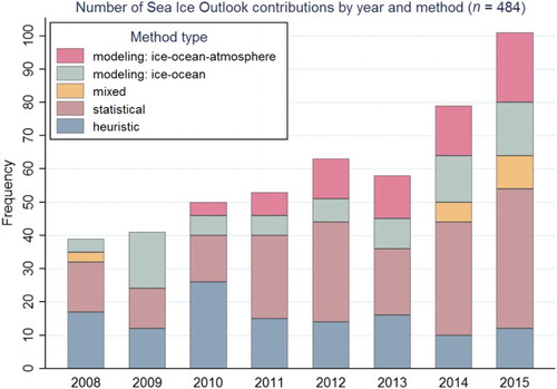
The overall upward trend in Figure 1 reflects a growing interest in Arctic sea ice both among scientists and the engaged public. Much of the growth came from modeling efforts, including ice-ocean-atmosphere models, reflecting increased contributions from operational centers.

Figure 2 visualizes one year of SIO contributions (2015), separating results by monthly cycle (early June, July and August) and type of method. Boxes indicate the median (50th percentile) and IQR (25th–75th percentile, which encloses roughly the middle 50% of each distribution). Predictions more than 1.5×IQR beyond the first or third quartile in each group are plotted individually as outliers. A horizontal line marks the observed 2015 September ice extent, 4.63 million km².

Figure 2. SIO June, July and August 2015 predictions for September mean sea ice extent. Box plots indicate the median, IQR and outliers for each distribution.

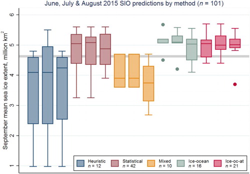
Heuristic methods, a diverse category that ranges from individual extrapolations to informal polls within science organizations, show a wide spread and include the lowest prediction by far, 1 million km². This low forecast was based on extrapolation of an earlier trend in sea ice extent and ice thickness. Other heuristic predictions were less extreme, but also generally came in lower than the observed September extent. These predictions often were based on spring-time ice thickness, concentration distributions or atmospheric conditions, but also include an informal pool of climate scientists. Mixed-method predictions were relatively few, but also tended toward underestimates.

The statistical and both modeling distributions are more populated and compact, although majorities in all three of these groups overestimated the observed extent. The median statistical prediction, unlike the median modeling predictions, moved slightly closer to the true value in August as some teams assimilated late information showing faster-than-expected melt. This partly reflects some modeling groups not updating outlooks with information available later in the summer. Only six modeling groups provided three distinct outlooks for June, July and August in 2015. It is also not clear if fully coupled configurations (ice-ocean-atmosphere) provide more accurate forecasts than forced configurations (ice-ocean). Interestingly, in 2014 the model predictions converged more closely on the observed extent as the season progressed. This suggests that initial conditions were perhaps less influential for the final extent in 2015 than in 2014.

The chaotic nature of the summer weather patterns plays a large role in the observed interannual variability in Arctic September sea ice extent (e.g. Guemas et al., 2014), determining the amount of sea ice melt and its movement. The 2015 SIO post-season report (SIPN, 2015b) notes how the outcome was affected by air pressure and weather events, which add to the challenge of predicting the final September ice extent:

Following the relatively cool May and June, the Arctic experienced one of the warmest Julys on record, which led to rapid ice loss through the month. The warm July was likely related to higher than normal sea level pressure over the central Arctic during the month … which indicates relatively clearer skies (and more incoming solar radiation). The high pressure over the Arctic was accompanied by lower pressure over northern Eurasia. This pattern helps funnel warm air into the Arctic from the south and compact sea ice into a smaller area. The rapid ice loss continued well into August and for a brief time it appeared that 2015 might surpass 2012’s record low extent. However, extent loss slowed considerably in late August and into September.

3. Easy and difficult years

Figure 3 graphs the observed September ice extent over the period for which we have satellite observation, 1979–2015 (National Snow and Ice Data Center [NSIDC], 2015). The quadratic regression curve shown here, which fits significantly better than a straight line, depicts an uneven but accelerating downward progression. Each year since 2007 had a September extent lower than any year before 2007. The unexpectedly abrupt drop in 2007, following decades of decline, heightened scientific concern about Arctic warming and gave impetus to launch SIO the next year. Toward lower right in Figure 3, squares mark the median July SIO prediction for each year (by all methods combined).

Figure 3. Observed September extent shown with quadratic trend and median of July SIO predictions, 1979–2015.

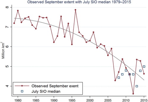
All of the SIO median predictions, like the observed ice extent, fall well below any pre-2007 values; in that respect they accurately reflect the general decline. In their year-to-year variations, however, median SIO predictions correlate with the previous year’s extent (R² = 0.90) rather than the year for which predictions are made (R² = 0.05). Figure 4 takes a closer look at the years since 2008, when SIO began. The jagged line connecting observed sea ice extent dots, and the squares representing median July SIO predictions, are the same as those in Figure 3. Vertical line segments added to Figure 4 show ensemble errors defined as observation minus median SIO prediction. Shading indicates the IQR or approximate middle 50% of individual predictions.

Figure 4. Observed September extent compared with median and IQR of July SIO predictions, 2008–2015.

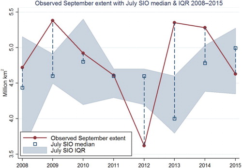
In four of these eight years (2009, 2012, 2013 and 2014), the errors are half a million km² or more, and observed extent falls outside the IQR of SIO predictions. In four other years the errors are smaller, and observed extent falls within this middle 50% of predictions. The conclusion that sea ice prediction has easy and difficult years was already observable in 2008–2013 and 2014 SIO data (Stroeve, Hamilton, et al., 2014b; Stroeve et al., 2015) and further confirmed with two datasets involving informal polls among scientists (Hamilton et al., 2014). All of these datasets identified 2009, 2012 and 2013 as difficult years to predict – in the sense that few if any predictions came close to the observed extent.

While the long-term downward trend in ice extent (Figure 3) in part reflects Arctic warming, with increased ice melting from the bottom and top (e.g. Perovich, Richter-Menge, Jones, & Light, 2008; Stroeve et al., 2012), in the ‘difficult’ years highlighted by Figure 4, unforecasted weather conditions steepened or halted this decline. For example, early-season indications in 2009 pointed toward the possibility of setting a new minimum record, and the median early-July SIO prediction was correspondingly low – 4.6 million km². But relatively cool weather in August and September slowed melting and left 5.38 million km² of ice, well above the previous two years. In 2012, an Arctic Dipole weather pattern (persistent high pressure over the Beaufort Sea and low pressure over the Kara Sea) in early June fueled expectations that extent would be relatively low, similar to the year before, so the median early-July SIO prediction was 4.6 million km². However, a large low-pressure storm in early August helped to break up ice floes, pushing them further south into warmer waters where they could melt, as well as increasing the mixing in the oceanic boundary layer that also led to increased bottom melting (Zhang, Lindsay, Schweiger, & Steele, 2013). Extent fell more than 2.7 million km² in one month, leading to a new September record of just 3.62 million km². SIO predictions were wrong by a similar amount in 2013, but in the opposite direction. The loss of so much multiyear ice in previous years, and especially 2012, led to expectations of another low extent. The median early-July SIO prediction consequently was 4 million km², just slightly higher than the year before. Persistent low pressure during summer, however, caused ice divergence and limited heat transport, keeping summer temperatures below normal over much of the Arctic Ocean. These factors resulted in a relatively large September extent, 5.35 million km².

4. Ensemble vs. naive predictions

Ease and difficulty in sea ice prediction correspond roughly to the distinction between climate and weather. Those years in which unusual weather conditions caused a sharp departure in sea ice extent, compared with the previous year, are also the years when SIO prediction errors are large. Figure 5 plots SIO ensemble errors, defined as observed September extent minus median July SIO prediction, against the change in the observed extent compared with the previous year. When there is a large change in sea ice extent compared with the previous year, the median SIO predictions are likely to be far off as well, and in the same direction. Change from the previous year explains 86%of the variance in SIO median errors.

Figure 5. SIO prediction error (median July SIO minus observed September extent) versus observed change from September the previous year, 2008–2015.

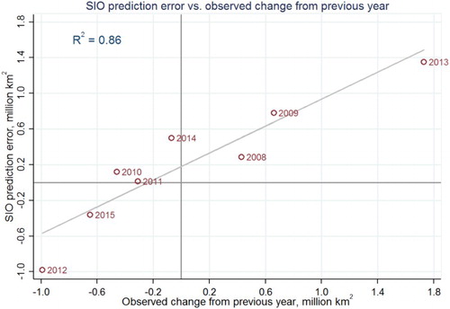
The strong correlation in Figure 5 suggests that expecting ‘persistence’, or guessing that this year’s ice extent will be the same as last year’s, might yield predictions competitive with the median SIO. An alternative, climatological null hypothesis could use predictions from either linear or quadratic extrapolation, representing the overall trends to that date. Table 1 compares the accuracy of these four strategies in terms of their root mean squared errors (RMSE) or their more outlier-resistant median absolute errors. By either criteria, the median SIO predictions perform better than guessing last year’s value, and at least moderately better than extrapolating the downward trend (whether linear or quadratic) up to but not including each year.

Table 1. Comparison of median July SIO predictions with predictions based on linear or quadratic extrapolation (using data from 1979 to the previous year) or persistence (extent same as previous year), over 2008–2015, in millions of km².

	RMSE	Median absolute error
SIO July median	0.696	0.432
Linear extrapolation	0.721	0.503
Quadratic extrapolation	0.739	0.480
Persistence	0.816	0.555

The RMSE and median absolute errors of Table 1 are in millions of km². Thus, taking the July SIO median as our prediction each year yields a median absolute error of 432,000 km². Although lower than the median absolute errors from linear extrapolation (503,000 km²), quadratic extrapolation (480,000 km²) or persistence (555,000 km²), that still leaves much room for improvement in predicting the interannual variations of sea ice extent.

5. Individual prediction errors

Although the SIO provides an archive of predictions by its contributors, it is not set up to evaluate the performance of specific methods or individual research teams. The methods used by one team can change in small or large ways between successive years or even within a season, as scientists refine their techniques. Consequently, researchers themselves are better positioned to judge how well they are doing, and to interpret their own SIO record. The SIO database does support evaluations of general method types, however, as these are applied across different months and years.

Table 2 gives results from three regression models testing year, month and method as factors that might affect the absolute errors of SIO predictions. The statistical technique employed here, quantile regression (Koenker, 2005), does not assume normality and has good resistance to outliers, making it better suited than ordinary least squares for the skewed, heavy-tailed SIO error distributions. Because the common regression assumptions of independent and identically distributed disturbances are implausible for these clustered data, we also use robust standard errors and t tests that do not require such assumptions. For each set of categorical predictors (year, month and method), one value is selected as a base or comparison category. ‘Base category’ is a statistical choice for interpretation, not affecting the overall fit of the models. Thus, 2014 is set as the base category of year, because prediction errors in that year were closest to the average for the dataset as a whole. June is the base category of month, in order to test whether July or August significantly improves on June. Heuristic is designated the base category of method. Regression coefficients in the table represent contrasts against these base categories, in millions of km², for any given combination of values for the other variables in each model.

Table 2. Quantile regression coefficients (with robust standard errors), modeling the median absolute prediction error as a function of (0,1) indicators for year, month and method. Base groups are the comparison categories. Regression 2 and 3 apply the new distinction between ice-ocean and ice-ocean-atmosphere modeling; regression 3 includes contributions only from researchers, setting aside those identified as general public.

	Regression
	1	2	3 (ex. public)
Year
2008	−.03 (.14)	−.01 (.14)	.00 (.14)
2009	.17 (.08)*	.19 (.07)*	.16 (.07)*
2010	−.16 (.11)	−.11 (.11)	−.14 (.12)
2011	−.30 (.09)***	−.28 (.09)**	−.31 (.09)***
2012	.24 (.10)*	.28 (.10)**	.29 (.10)**
2013	.67 (.13)***	.71 (.11)***	.73 (.11)***
2014	Base	Base	Base
2015	−.04 (.08)	−.01 (.08)	−.05 (.07)
Month
June	base	base	base
July	.03 (.05)	.01 (.04)	.00 (.04)
August	−.10 (.05)	−.08 (.05)	−.06 (.05)
Method
Heuristic	Base	Base	Base
Modeling	−.10 (.06)	…	…
Statistical	−.15 (.06)*	−.15 (.05)**	−.10 (.06)
Mixed	.09 (.20)	.07 (.20)	.16 (.22)
Ice-ocean	…	−.09 (.05)	−.00 (.05)
Ice-ocean-at	…	−.17 (.08)*	−.13 (.08)
constant	.68 (.09)***	.67 (.08)***	.62 (.08)***
estimation sample	484	484	429

*p < .05; **p < .01; ***p < .001 t tests using robust standard errors.

Regression 1 employs the original classification with four broad method types: heuristic (set as the base category), modeling, statistical or mixed. Regression 2 employs the newer scheme with five types, which separates the modeling group into ice-ocean and ice-ocean-atmosphere models. Regression 3 is the same as 2, but with estimation restricted only to SIO predictions by researchers, setting aside 55 general-public contributions.

Coefficients for each year term represent the difference between the median absolute error in that year compared with 2014. Positive coefficients therefore indicate years with larger-than-2014 errors. Median absolute errors in 2009, 2012 and 2013 are significantly greater than 2014 across all three regression models. In regression 1, for example, the median absolute errors in these years exceed that of 2014 by 170,000 to 670,000 km². In 2011 on the other hand, median absolute errors were about 300,000 km² less than in 2014. As graphed in Figure 4, the median July SIO prediction in 2011 almost exactly equaled the observed September extent.

Coefficients on the month terms in Table 2 contrast the median absolute error for July or August with that for June, the base category. Median absolute August errors are slightly lower than June, but these differences are not statistically significant.

Heuristic methods provide our base category among method terms, so coefficients compare the heuristic errors with those of modeling, statistical or mixed-method groups. Regressions 2 (all contributions) and 3 (setting aside general-public contributions) apply the new distinction among modeling efforts: those based on ice-ocean models, or more complex models that encompass the atmosphere as well. Statistical methods and ice-ocean-atmosphere models both perform significantly better (by 150,000–170,000 km²) than heuristic methods in the full dataset of SIO predictions (regression 2). If we set aside contributions from the general public, however, the contrasts between statistical or ice-ocean-atmosphere modeling and the remaining heuristic predictions become smaller (100,000–130,000 km²), falling short of statistical significance (regression 3).

6. Discussion

Sea ice predictions lag meteorological predictions by several decades (Jung et al., 2016), and the use of dynamical models to forecast real-word sea ice conditions is just now gaining traction (Blanchard-Wrigglesworth, Cullather, Wang, Zhang, & Bitz, 2015). Nevertheless, several studies have examined limits of sea ice predictability in dynamical models, reflecting a growing interest in developing reliable methods for seasonal ice forecasting. While the current SIOs offer only limited improvement over the naïve hypotheses of persistence, or extrapolation from linear or quadratic trends, studies have suggested high skill is possible for retrospective predictions of the pan-Arctic sea ice extent up to 6 months in advance (e.g. Massonnet, Fichefet, & Goose, 2015; Msadek, Vecchi, Winton, & Gudgel, 2014). Even longer lead times may also be possible based in part on memory of sea ice thickness and ocean conditions (e.g. Blanchard-Wrigglesworth, Bitz, & Holland, 2011; Chevallier & Salas-Melia, 2012; Day, Hawkins, & Tietsche, 2014). One thing that has become clear is that better observations, such as sea ice thickness (Day et al., 2014) and model improvements (e.g. Blanchard-Wrigglesworth et al., 2015; Juricke, Goessling, & Jung, 2014), could raise predictive skill. Making better use of existing satellite-based observations of ice thickness, such as those from CryoSat-2 (Laxon et al., 2013), SMOS (Kaleschke, Tian-Kunze, Maass, M¨akynen, & Drusch, 2012) and the planned ICESat-2 mission (Kwok, 2010), therefore may be a way forward in improving forecast skill. There is also promise in using IceBridge aircraft flight lines of ice thickness to initialize forecasts (Lindsay et al., 2012).

Nevertheless, it is somewhat surprising that the SIO accuracy has not improved substantially over these eight years. This may in part reflect the sensitivity of a thinner ice cover to anomalous weather conditions as the Arctic Ocean has transitioned from being dominated by multiyear ice to seasonal ice. The multiyear ice that has remained is also younger and thinner (e.g. Comiso, 2012; Haas et al., 2008). During a thinner ice regime, an unusually warm summer has the potential to result in large reductions in ice extent whereas in a thicker ice regime, the ice is still thick enough to not melt out entirely. Conversely, during a cooler than normal summer, survival of ice will translate into a larger overall extent, even if that ice is very thin. At the same time, thinner ice is more easily ridged and transported by winds (Rampal, Weiss, Marsan, & Bourgoin, 2009). This increased sensitivity of the sea ice extent to summer atmospheric forcing as the ice cover has thinned (e.g. Holland, Bailey, & Vavrus, 2010) may be one factor holding back predictability, though it remains unclear how this regime shift has influenced individual prediction methods. Many statistical models, as well as dynamical models treat ice dynamics and thermodynamics based on regressions determined from past system behavior (statistical models) or parameterizations (dynamical models) developed when the Arctic was a multiyear ice regime. These formulations may no longer be valid in the new first-year ice regime. Another complication with regard to ice-ocean models forced with atmospheric reanalysis is that the statistics of past forcing fields may no longer be applicable in the new Arctic state. This is one reason why many of the coupled ice-ocean model contributions use ensembles from the last decade rather than the entire satellite data record.

Improvements in sea ice forecasting and model initialization will likely improve also weather forecasts at lower latitudes (Jung, 2016). For example, Stroeve and Notz (2015) note that the forecast of air temperature depends strongly on the sea ice concentration, such that initializing a forecast with NASA Team (Cavalieri, Gloersen, & Campbell, 1984) or Bootstrap (Comiso, 1986) derived May sea ice concentrations might cause regional differences of more than 3°C in simulated September air temperatures. Further, the timing of when the ice returns in the autumn/winter affects Arctic air temperatures that may in turn impact winter climate and weather extremes at lower latitudes (e.g. Francis & Vavrus, 2012). The atmospheric response to sea ice could influence sea ice predictability because persistent atmospheric planetary-scale waves are also sources of predictability.

The newly opened areas and extended marginal ice zones in the Arctic provide new opportunities for shipping, tourism, offshore resource extraction (e.g. Stephenson, Smith, Brigham, & Agnew, 2013) while at the same time increase risks for coastal communities in terms of increased exposure to waves and storm surges and coastal erosion (e.g. Hamilton et al., 2016; Khon et al., 2014). Reliable forecasts of summer conditions a few months in advance would prove highly useful for anticipating how long the ocean areas will be ice-free each year.

7. Conclusions

An earlier examination of the SIO through 2013 noted a dominant pattern of easy and difficult years, which eclipsed smaller differences in ensemble skill among method types, and improvements by month within each melting season (Stroeve, Hamilton, et al., 2014). Our analysis here extends earlier work through the inclusion of two further years with 180 additional SIO predictions; a new distinction (suggested by contributors) between ice-ocean and ice-ocean-atmosphere modeling methods and comparisons of SIO ensemble accuracy against naïve hypotheses based on persistence, linear or curvilinear extrapolation. We find that the median SIO predictions outperform naïve predictions, although sometimes not by wide margins. Ice-ocean-atmosphere models and statistical prediction methods do somewhat better, collectively, than predictions based on other method types. Early-August predictions, as a whole, show very modest improvement compared with June or July predictions. The strongest results from our 2008–2015 analysis confirm an earlier finding: sea ice prediction continues to show easy and difficult years. The easy/difficult pattern corresponds to the balance between climate (e.g. preconditioning; long-term trends) and weather influencing the outcome each year. The sensitivity to weather observed in these SIO years may itself reflect our present transitional era between an historical Arctic cool enough to retain much thick, resistant multiyear ice, and a warmed future Arctic where little ice remains at summer’s end.

Acknowledgements

Helen Wiggins and Betsy Turner-Bogren (ARCUS) provided SIO data.

Disclosure statement

No potential conflict of interest was reported by the authors.

ORCiD

Lawrence C. Hamilton http://orcid.org/0000-0003-1977-0649

Julienne Stroeve http://orcid.org/0000-0001-7316-8320

Additional information

Funding

This research was carried out under the SIPN project, with support from the US National Science Foundation (PLR-1303938) and the Office of Naval Research (N00014-13-1-0793).

References

- Blanchard-Wrigglesworth, E., Bitz, C. M., and Holland, M. M. (2011). Influence of initial conditions and climate forcing on predicting Arctic sea ice. Geophysical Research Letters, 38(18). doi:10.1029/2011GL048807
- Blanchard-Wrigglesworth, E., Cullather, R. I., Wang, W., Zhang, J., & Bitz, C. M. (2015). Model forecast skill and sensitivity to initial conditions in the seasonal Sea Ice Outlook. Geophysical Research Letters, 42(19), 8042–8048. doi:10.1002/2015GL065860
- Cavalieri, D. J., Gloersen, P., & Campbell, W. J. (1984). Determination of sea ice parameters with the NIMBUS-7 SMMR. Journal of Geophysical Research: Atmospheres, 89(D4), 5355–5369. doi: 10.1029/JD089iD04p05355
- Chevallier, M., & Salas-Melia, D. (2012). The role of sea ice thickness distribution in the Arctic sea ice potential predictability: A diagnostic approach with a coupled GCM. Journal of Climate, 25, 3025–3038. doi:10.1175/JCLI-D-11-00209.1
- Comiso, J. C. (1986). Characteristics of Arctic winter sea ice from satellite multispectral microwave observations. Journal of Geophysical Research, 91. doi:10.1029/JC091iC01p00975
- Comiso, J. C. (2012). Large decadal decline of the Arctic multiyear ice cover. Journal of Climate, 25, 1176–1193. doi: 10.1175/JCLI-D-11-00113.1
- Day, J., Hawkins, E., & Tietsche, S. (2014). Will Arctic sea ice thickness initialization improve seasonal forecast skill? Geophysical Research Letters, 41, 7566–7575. doi:10.1002/2014GL061694
- Emmerson, C., & Lahn, G. (2012). Arctic opening: Opportunity and risk in the high North. Chatham House-Lloyd’s Risk Insight Report. Retrieved from https://www.chathamhouse.org/publications/papers/view/182839#
- Francis, J. A., & Vavrus, S. J. (2012). Evidence linking Arctic amplification to extreme weather events in the mid-latitudes. Geophysical Research Letters, 39, n/a–n/a. doi:10.1029/2012GL051000
- Guemas, V., Blanchard-Wrigglesworth, E., Chevallier, M., Day, J. J., Deque, M., Doblas-Reyes, F. J., … Tietsche, S. (2014). A review on Arctic sea ice predictability and prediction on seasonal-to-decadal timescales. Quarterly Journal of the Royal Meteorological Society, 142, 546–561. doi:10.1002/qj.2401
- Haas, C., Pfaffling, A., Hendricks, S., Rabenstein, L., Etienne, J.-L., & Rigor, I. (2008). Reduced ice thickness in Arctic Transpolar drift favors rapid ice retreat. Geophysical Research Letters, 35, L107501. doi:10.1029/2008GL034457
- Hamilton, L. C., Bitz, C. M., Blanchard-Wrigglesworth, E., Cutler, M., Kay, J., Meier, W., … Wiggins, H. (2014). Sea ice prediction has easy and difficult years. Witness the Arctic Spring, 3–7. Fairbanks, AK: Arctic Research Consortium of the U.S. Retrieved January 19, 2016, from http://www.arcus.org/witness-the-arctic/2014/2/article/21066
- Hamilton, L. C., Saito, K., Loring, P. A., Lammers, R. B., & Huntington, H. P. (2016). Climigration? Population and climate change in Arctic Alaska. Population and Environment. doi:10.1007/s11111-016-0259-6
- Holland, M. M., Bailey, D. A., & Vavrus, S. (2010). Inherent sea ice predictability in the rapidly changing Arctic environment of the community climate system model, version 3. Climate Dynamics, 36, 1239–1253. doi:10.1007/s00382-010-0792-4
- Jung, T., Gordon, N. D., Bauer, P., Bromwich, D. H., Chevallier, M., Day, J. J., … Yang, Q. (2016). Advancing polar prediction capabilities on daily to seasonal time scales. Bulletin of the American Meteorological Society. doi: 101175/BAMS-D-14-00246.1
- Juricke, S., Goessling, H. F., & Jung, T. (2014). Potential sea ice predictability and the role of stochastic sea ice strength perturbations. Geophysical Research Letters, 41, 8396–8403. doi:10.1002/2014GL062081
- Kaleschke, L., Tian-Kunze, X., Maass, N., M¨akynen, M., & Drusch, M. (2012). Sea ice thickness retrieval from SMOS brightness temperatures during the Arctic freeze-up period. Geophysical Research Letters, 39, n/a–n/a. doi:10.1029/2012GL050916
- Khon, V. C., Mokhov, I. I., Pogarskiy, F. A., Babanin, A., Dethloff, K., Rinke, A., … Matthes, H. (2014). Wave heights in the 21st century Arctic Ocean simulated with a regional climate model. Geophysical Research Letters, 41, 2956–2961. doi:10.1002/2014GL059847
- Koenker, R. (2005). Quantile regression. New York: Cambridge University Press.
- Kwok, R. (2010). Satellite remote sensing of sea ice thickness and kinematics: A review. Journal of Glaciology, 56, 1129–1140. doi: 10.3189/002214311796406167
- Laxon, S. W., Giles, K. A., Ridout, A. L., Wingham, D. J., Willatt, R., Cullen, R., … Davidson, M. (2013). CryoSat-2 estimates of Arctic sea ice thickness and volume. Geophysical Research Letters, 40(4), 732–737. doi:10.1002/grl.50193
- Lindsay, R., Haas, C., Hendricks, S., Hunkeler, P., Kurtz, N., Paden, J., … Zhang, J. (2012). Seasonal forecasts of Arctic sea ice initialized with observations of ice thickness. Geophysical Research Letters, 39(21), n/a–n/a. doi:10.1029/2012GL053576B
- Massonnet, F., Fichefet, T., & Goose, H. (2015). Prospects for improved seasonal Arctic sea ice predictions from multivariate data assimilation. Ocean Modelling, 88, 16–25. doi: //10.1016/j.ocemod.2014.12.013
- Msadek, R., Vecchi, G., Winton, M., & Gudgel, R. (2014). Importance of initial conditions in seasonal predictions of Arctic sea ice extent. Geophysical Research Letters, 41, 5208–5215. doi:10.1002/2014GL060799
- National Snow and Ice Data Center. (2015). Sea ice index. National Snow and Ice Data Center. Retrieved February 1, 2016, from https://nsidc.org/data/seaice_index/
- Perovich, D. K., Richter-Menge, J. A., Jones, K. F., & Light, B. (2008). Sunlight, water and ice: Extreme Arctic sea ice melt during the summer of 2007. Geophysical Research Letters, 35, L11501. doi:10.1029/2008GL034007
- Rampal, P., Weiss, J., Marsan, D., & Bourgoin, M. (2009). Arctic sea ice velocity field: General circulation and turbulent like fluctuations. Journal of Geophysical Research, 114, C10014. doi:10.1029/2008/C005227
- Sea Ice Prediction Network. (2015a). Sea ice outlook. Arctic Research Consortium of the U.S. Retrieved February 1, 2016, from https://www.arcus.org/sipn/sea-ice-outlook
- Sea Ice Prediction Network. (2015b). September Sea ice outlook: Post-season report. Arctic Research Consortium of the U.S. Retrieved February 1, 2016, from https://www.arcus.org/sipn/sea-ice-outlook/2015/post-season
- Sea Ice Prediction Network. (2016). SIPN: Sea ice prediction network. Arctic Research Consortium of the U.S. Retrieved March 4, 2016, from https://www.arcus.org/sipn
- Simmonds, I. (2015). Comparing and contrasting the behaviour of Arctic and Antarctic sea ice over the 35 year period 1979–2013. Annals of Glaciology, 56(69), 18–28. doi:10.3189/2015AoG69A909
- Stephenson, S. R., Smith, L. C., Brigham, L. W., & Agnew, J. A. (2013). Projected 21st-century changes to Arctic marine access. Climatic Change, 118(3), 885–899. doi:10.1007/s10584-012-0685-0
- Stroeve, J., Blanchard-Wrigglesworth, E., Guemas, V., Howell, S., Massonnet, F., & Tietsche, S. (2015). Improving predictions of Arctic sea ice extent. Eos, 96. doi:10.1029/2015EO031431
- Stroeve, J., Hamilton, L. C., Bitz, C. M., & Blanchard-Wrigglesworth, E. (2014). Predicting September sea ice: Ensemble skill of the SEARCH Sea ice outlook. Geophysical Research Letters, 41, 2411–2418. doi:10.1002/2014GL059388
- Stroeve, J. C., Markus, T., Boisvert, L., Miller, J., & Barrett, A. (2014). Changes in Arctic melt season and implications for sea ice loss. Geophysical Research Letters, 41(4), 1216–1225. doi:10.1002/2013GL058951
- Stroeve, J., & Notz, D. (2015). Insights on past and future sea-ice evolution from combining observations and models. Global and Planetary Change, 135, 119–132. doi:10.1016/j.gloplacha.2015.10.011
- Stroeve, J. C., Serreze, M. C., Kay, J. E., Holland, M. M., Meier, W. N., & Barrett, A. P. (2012). The Arctic’s rapidly shrinking sea ice cover: A research synthesis. Climatic Change, 110(3), 1005–1027. doi:10.1007/s10584-011-0101-1
- Study of Environmental Arctic Change. (2016). SEARCH: Study of Environmental Arctic Change. Arctic Research Consortium of the U.S. Retrieved March 4, 2016, from https://www.arcus.org/search-program
- Zhang, J., Lindsay, R., Schweiger, A., & Steele, M. (2013). The impact of an intense summer cyclone on 2012 Arctic sea ice retreat. Geophysical Research Letters, 40(4), 720–726. doi:10.1002/grl.50190